1. Introduction
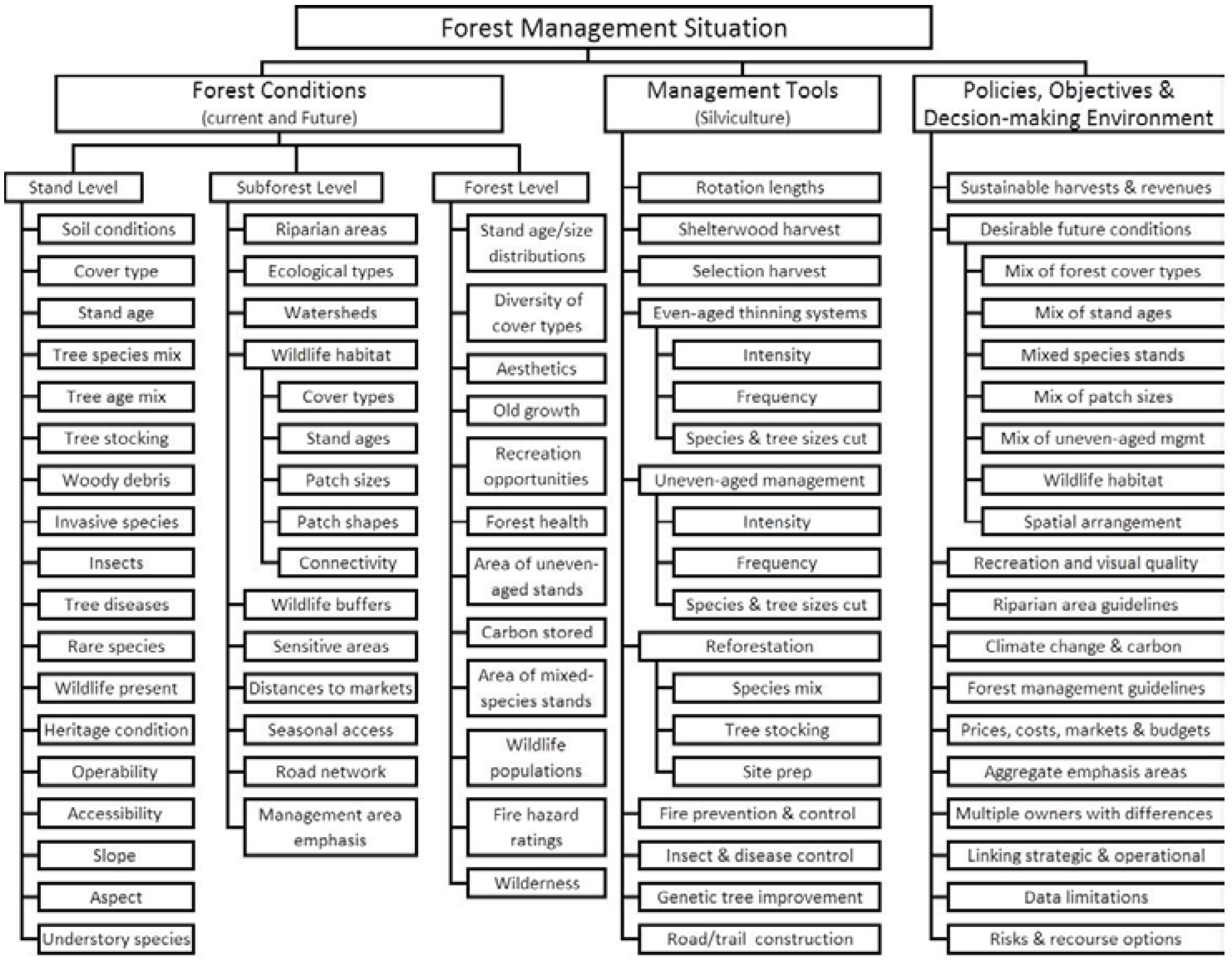
Forest management situations are typically complex, multi-faceted problems. Decisions often must be made to incorporate broad landscape level objectives such as wildlife population needs, forest health, and sustainable harvest; it is also important to recognize stand-level details such as soil conditions, mixed tree species and/or ages, or operability (
Figure 1). Also, long planning horizons are generally needed, and many forests are mosaics of multiple ownerships. Managers want to understand the trade-offs associated with the management options available. The integration of ecological and economic objectives is considered one of the biggest hurdles for forest planning. The consequences resulting from forest management decisions made today will likely affect landscape conditions and associated ecosystem services far into the future.
The concept of ecosystem services was developed to address the linkages between ecosystems and human well-being. Ecosystem services are defined as the benefits that people obtain from ecosystems [
1]. Due to the diversity and complexity of ecosystems and associated ecosystem services, an interdisciplinary effort is generally needed. A key in studying ecosystem services is in combining economics and ecology [
2]. Gómez-Baggethun et al. presents the history of how economic theory has considered nature’s benefits from a classic economic perspective up through a modern view of ecosystem services [
3].
Ecosystems reinforce human well-being in many ways, and this fact is acknowledged in the Millennium Ecosystem Assessment, where ecosystem services are divided into provisioning (food, fresh water, fuel, timber,…), regulating (climate regulation, erosion regulation, water quality,…), cultural (recreational, aesthetic, spiritual values,…), and supporting services (soil formation, nutrient cycling,…) [
1]. Both the definition and classification stated in the Millennium Ecosystem Assessment have been widely used, but other definitions and classifications of ecosystem services are highlighted in the literature [
5,
6,
7,
8]. Fisher et al., as well as Boyd and Banzhaf, argued the need to distinguish between intermediate services (considered as processes or functions in Boyd and Banzhaf) and final ecosystem services, to avoid double counting services when estimating their economic values, aggregating their values, or integrating them into a model [
9,
10]. They also discriminated between services and benefits, advocating that services are benefit-specific [
10] and that the same service can produce several benefits [
9]. Boyd and Banzhaf suggested to define final ecosystem services as the components of nature or ecological characteristics that are directly used or consumed to produce human well-being, they are nature’s end-products. However, Fisher et al. promoted the idea of considering ecosystem services as the aspects of the ecosystem that are either actively or passively used to produce human well-being [
9].
Additionally, Fisher et al. also discussed the use of the relationships between supply and demand of ecosystem services to evaluate and connect them to human welfare [
9]. This economic framework highlights the idea that the willingness to pay for an ecosystem service might not always be constant, depending on both the quantity and quality of the ecosystem service provided. In other words, the value of an ecosystem service is a function of marginal changes in the flow of the service produced. The marginal value could also be understood as the amount that people are willing to pay to access to an extra unit of the service or the price that people would pay to avoid losing one unit. With this approach, higher marginal values will be assigned to an ecosystem service when it becomes scarce, and this marginal value will decrease as the supply of the service increases. In other words, the value of additional services will depend on the level of ecosystem service already provided.
In the case of forest ecosystems, the list of services that humans can benefit from is very extensive, ranging from timber production, water regulation (quality and quantity), carbon storage, local and global climate regulation, nontimber products, or wildlife habitat. Binder et al. [
11] present a detailed review of forest ecosystem services highlighting research related to ecological production functions and economic benefits functions for the different forest uses. Old forest is considered an ecological end product that could provide several benefits including wildlife habitat, recreational use, biological diversity, and/or aesthetic value. The old forest definition should not be confused with the old growth stage (or multi-aged complex [
12]) of stand development, which is classified based on structure, composition, and function. The age at which a stand provides old forest services may vary by region due to differences in climate and species. For example, in northern Minnesota, USA, many of the common species are early successional with average life spans of less than 150 years [
13]. This may be very different from other regions, for example rotations shorter than 10 years for eucalypt species (
Eucalyptus spp.) in Brazil [
14] versus cutting cycles where the maximum age of Engelmann spruce (
Picea engelmannii Parry ex Engelm.) can be greater than 300 years in the Intermountain West in the USA [
15]. An important reason that age is used to define old forests is that it can be more easily assessed and used by forest planning models compared to structure, composition, and function.
The Multiple Use Sustained Yield Act of 1960 (P.L. 86–517) requires US national forests to be managed for outdoor recreation, range, timber, watershed, and wildlife, and fishing purposes. The National Forest Management Act (NFMA) of 1976 (P.L. 94–588) requires the USDA Forest Service to use a systematic and interdisciplinary approach to management planning. Forest planning models integrating multiple forest uses have been used since the 1970s. Work has ranged from developing general models that account for the production of multiple services [
16], to specific models accounting for timber and wildlife production, including both spatial and temporal dimensions [
17,
18] or models that provide an even flow of timber production while minimizing sediment levels settled to stream segments [
19]. Diaz-Balteiro and Romero extensively reviewed the most recent forest management problems with a multiple criteria decision making approach [
20]. In addition, Filyushkina et al. compiled and analyzed the most recent studies that integrate non-market forest ecosystem services into the decision making in the Nordic countries [
21]. Borges et al. provides good detail on the role of scheduling models in forest management [
22]. Downward-sloping demand (marginal value) curves have been explored and used in forestry, primarily for timber production [
23,
24,
25,
26].
Even though studies related to ecosystem services might differ on how they define and classify the services that multi-functional ecosystems provide, there is a common conclusion that both the economic valuation of ecosystem services and understanding benefits and costs of management options are key to help make decisions when managing ecosystems. We also want to acknowledge that forest management is intrinsically a joint production problem. Decisions made with the interest of producing a specific ecosystem service may affect the production of other forest ecosystem services.
With the main goal of understanding better the trade-offs of integrating multiple ecosystem services we study a harvest scheduling model considering the combined production of two ecosystem services: timber and old forest production. We use the marginal valuation approach described above to value the old forest service. Emphasis is made on important details, including stand-level differences in the forest cover type, stand age, ecological region, site quality, riparian percent, and distances to timber markets. We use an application of the model in northern Minnesota in the US to help us better understand the impact of incorporating multiple ecosystem services into the decision-making process. There is a wide range of factors that can impact the quantity and quality of old forest, such as forest cover type, intensity of harvest levels of the main forest cover types, stand ownership, ecological region, and the successional nature of the cover type among others. With the purpose of understanding the relationship between all these factors and the production of the old forest, we analyzed (1) the production of upland hardwood old forest under different forest management options, (2) the trade-offs of using distinct marginal value functions for the production of old forest, and (3) the potential impacts of adding premium values to major forest land ownership groups to produce old forest. As it is often done in forest planning, multiple model scenarios are emphasized with comparisons across scenarios adding insight on trade-offs and impacts of modeling assumptions.
2. Materials and Methods
We explained our study methods in four steps. First, we provided an overview of the forest management situation in northern Minnesota with a desire for a landscape approach for analysis considering all forest landowners. Next, we described an overview of the forest management scheduling model used, with its ability to decompose large problems to help recognize important forest details. Then, we provided background on a marginal approach for valuing old forest over time with a multi-ownership landscape perspective, and described alternative scenarios modeled to address old forest for the Minnesota situation. Finally, we described details on additional facets modeled to help address impacts of plausible changes in timber demands and opportunities to recognize quality differences in terms of the old forest produced.
2.1. Overview of the Forest Management Situation in Minnesota
The state of Minnesota is located in the north-central portion of the United States and is bordered by Canada to the north. Approximately 35% of the 22.5 million hectares of Minnesota is classified as forested [
27]. The forests of Minnesota are diverse and include three of Bailey’s ecosystem provinces: Prairie Parkland in the west, the Eastern Deciduous Forest through the center and southeastern section, and the Laurentian Mixed Forest in the northeast [
28]. The past glacial activity has substantially shaped topography and soil condition across the state, generating a low topographic relief landscape and a broad selection of soil conditions ranging from sandy outwash plains to rich peat bogs [
29]. The soil composition has influenced vegetation cover, resulting in pine (
Pinus) species commonly observed on sandier less nutrient-rich soils, hardwoods observed on nutrient-rich silt loams, and spruce (
Picea), tamarack (
Larix), and ash (
Fraxinus) species observed in poorly drained bogs. In addition, past human actions have also had a large effect on the current forest cover in Minnesota. Agricultural conversion and intensive logging practices during the late 19th and early 20th centuries have greatly influenced current forest distribution and composition [
29].
Ownership is diverse and includes multiple forest management agencies including the USDA Forest Service, the Minnesota Department of Natural Resources (DNR), county land departments, Tribal governments, industrial private landowners, and non-industrial private landowners. Management objectives frequently vary by owner. Among public land, state and county lands are more intensely managed for timber production [
30]. A state requirement of both state and county lands is the production of timber for revenue, some of which is used to help fund schools in the local communities. Of the federal lands, the Superior National Forest’s Boundary Water Canoe Area Wilderness (BWCAW), with an approximate extent of 400,000 hectares, is part of the National Wilderness Preservation System, and it is reserved forest land which is not available for timber production.
This study utilized information generated from a recent and ongoing Minnesota study [
31]. Data needs were intensive and included forest inventory data, forest inventory projections, cost estimates of silvicultural treatment options, and timber transportation cost estimates to major timber market centers in Minnesota. USDA Forest Inventory and Analysis (FIA) inventory data was used to describe and help project the forestlands in the model. The Minnesota DNR has aggregated the USDA Forest Service forest cover type classifications into 11 Minnesota forest cover types. We used that classification with a few small modifications. Aspen is the main forest cover type in Minnesota (29% of the statewide forest land), followed by black spruce (9%), oak (9%), northern hardwoods (9%), and lowlands hardwoods (9%) [
30]. The aspen forest cover type is also widely spread across the study area. It usually contains a substantial component of other species, with the mix generally containing more hardwoods in the Southwest and more conifers in the Northeast. FIA data are collected using a nationally consistent two-phase sampling design and the program uses an annual system in which all the field plots are visited and measured once during the survey cycle. The duration of that cycle is five years in Minnesota, therefore one-fifth of the forestland is measured every year. The spatial sampling intensity of the FIA program in Minnesota is close to one plot per 2428 hectares [
32,
33]. Data from the FIA program are available and open to the public. The sampling design of the FIA plots allows them to be further divided into ‘conditions’, meaning that a proportion of a plot could be in different forest condition. This could be based on differences in the forest cover type, ownership, stand age, or reserve status. Data for this study were collected for the 2010–2014 survey cycle. A total of 7169 of FIA plots were included, characterizing approximately 6,046,840 hectares of forest land in Minnesota that are north of the Minneapolis-St. Paul metropolitan area, about 95% of the forest land in Minnesota.
Separate AAs were used for each of all of the forest condition classes of FIA plots in the study area. Each FIA plot condition class was subdivided to reflect estimated areas in one of three riparian classes. Each FIA condition class on privately-owned land was further subdivided into five classes to reflect timing assumptions regarding the availability for harvest. Details are described in Hoganson et al. [
31] with availability assumptions generally varying by stand age and forest cover type.
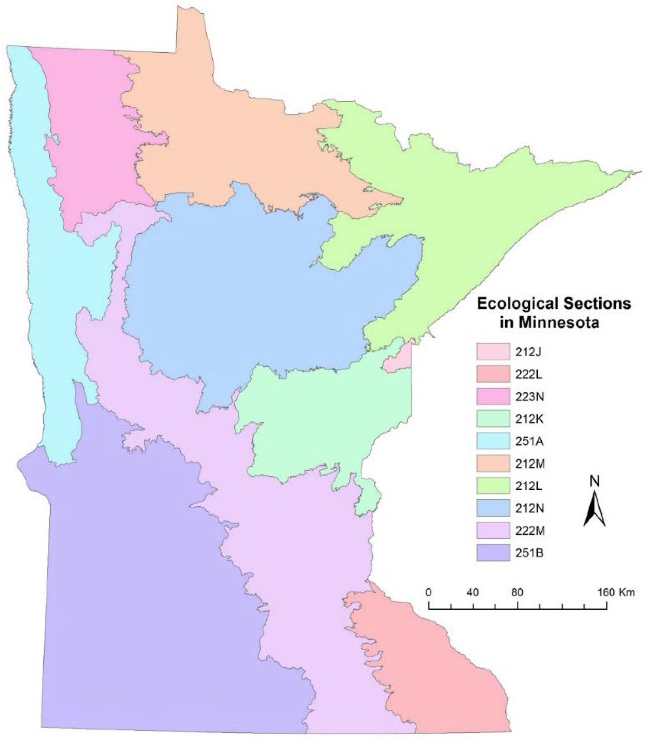
Aspen and red pine (
Pinus resinosa Ait.) are two of the most valuable tree species for the forest industry and with the highest demand in Minnesota. To help account for regional variation of the aspen forest cover type in Minnesota, the AAs in the aspen cover type are further classified based on ecological region (
Figure 2). Tree species mixes found in aspen stands vary substantially by ecological region, as do natural succession cover type pathways of stands currently in the aspen forest cover type. Red pine AAs were subdivided into red pine plantations and natural stands of red pine, allowing the model to recognize higher yields and thinning opportunities from red pine plantations.
In addition to clearcut options for harvest, shelterwood systems were considered for oak, and uneven-aged management options were considered for northern hardwoods. No-harvest options were considered for all AAs. Although old forest objectives are of concern for all forest cover types, this study focused on old forest production of hardwoods on uplands. Northern hardwoods in Minnesota is a mix species cover type commonly constituted by red maple (Acer rubrum), sugar maple (Acer saccharum), paper birch (Betula papyrifera), trembling aspen (Populus tremuloides), northern red oak (Quercus rubra), and basswood (Tilia Americana).
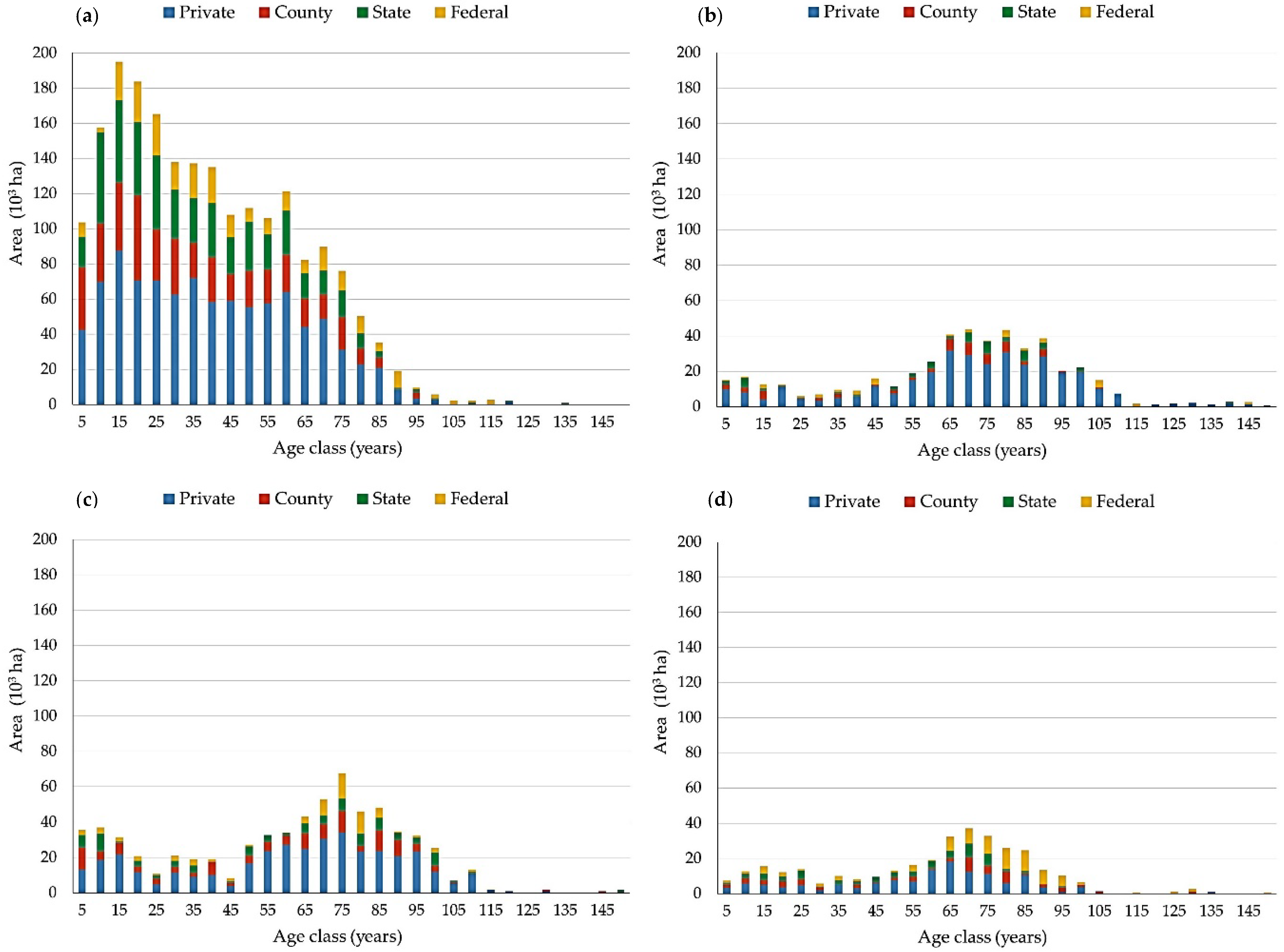
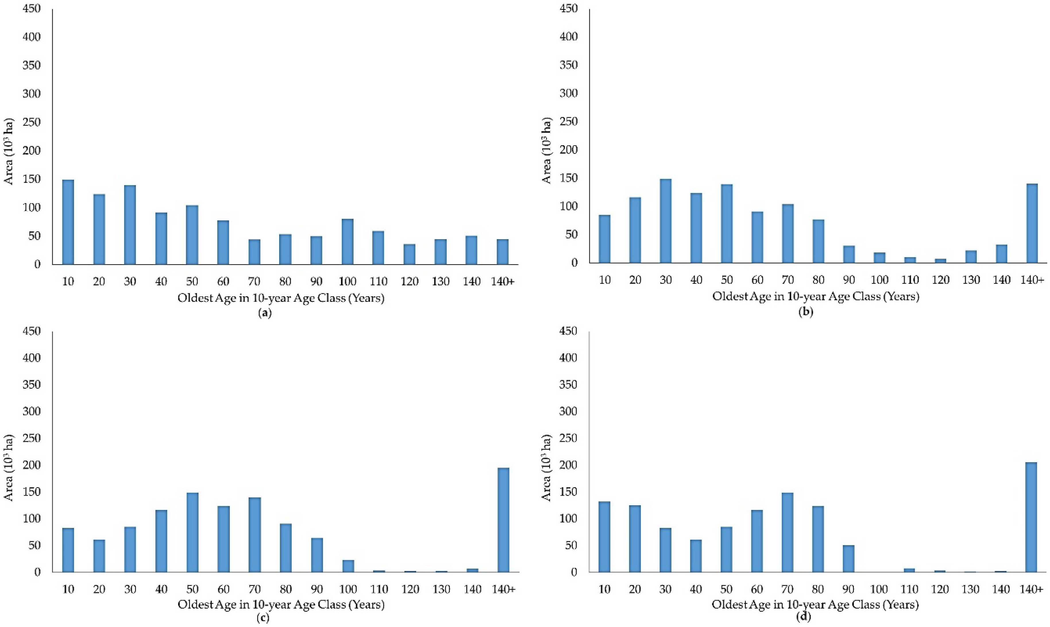
To help the reader understand better the current situation for the study area,
Figure 3 shows, by forest ownership, the age-class distributions for the main cover types at the start planning horizon. In Minnesota, optimal economic rotation age for the aspen cover type is usually 40–45 years, 80–90 years for the oak and northern hardwoods cover types depending on site quality, and 50 years for the birch cover type.
Figure 3 illustrates the current relative abundance of financially overmature imbalance for both aspen and birch cover types for timber production at the start of the planning horizon, as well as, the fact that the majority of the oak and northern hardwoods timberland are on private lands. The graphs also use the same scale, helping illustrate the current balance of these four forest cover types central to this study.
2.2. Dualplan: Background and Overview of the Model
Dualplan is a forest management scheduling model developed initially over 30 years ago [
34]. Over time it has been substantially updated with diverse features and modules that give the model flexibility to describe and track important stand-level detail while addressing relatively large problems [
35,
36,
37,
38,
39,
40]. Dualplan and Dtran, its multi-market, multi-ownership, transportation variant, have been successfully applied in many large studies, ranging from all-landowner-multi-market studies emphasizing timber based economic development [
41,
42] to USDA National Forest planning emphasizing spatial arrangement of the forest for wildlife habitat [
43,
44,
45,
46].
Dualplan uses a Model II linear programming formulation [
47] to define the forest planning problem. It decomposes the formulation into subproblems that are each linked to the master problem via the dual variables associated with the forest-level constraints of the master problem. Forest-level constraints can range from constraints on total timber production by planning period to periodic targets for old forest characteristics. In the simplest case, each subproblem in Dualplan is an economic analysis of a specific timber stand. Analyses for each subproblem use estimated values of dual variables for the forest-wide constraints of the master problem to recognize the stand-level impacts of stand management options on the forest-wide constraints [
34,
48,
49]. Once Dualplan develops an initial forest-wide schedule, the schedule is summarized with those results used to help re-estimate the optimal values of the dual variables for the forest-wide constraints. The subproblem solution process is repeated iteratively, each time updating estimates of the dual variables (shadow prices) for the forest-level constraints. With its ties to duality theory, the solution process always produces optimal solutions, yet the solutions are infeasible solutions in that they typically violate at least some of the forest-wide constraints of the master problem. However, the process of using the intermediate results to help re-estimate the values of the dual variables is key to help move solutions towards feasibility. Applications have consistently found that estimates of the dual variables for the forest-wide constraints can be determined such that violations (infeasibilities) of the forest-wide constraints are acceptable in practical terms. With its ability to decompose problems into subproblems, very detailed forest-wide problems (many stands) can be addressed.
Dual variable value estimates (shadow price estimates) are central for addressing forest-level constraints in stand-level analyses. Essentially, each dual variable value estimate is an added bonus or penalty to include in a stand-level analysis so that forest-level impacts of stand-level management options are addressed when they are evaluated. The level of these bonuses or penalties is often valuable information to decision-makers in selecting appropriate constraint levels (targets) for the forest-level constraints. Often a key aspect of planning is to use the analyses to help select targets or goals for the forest as more is learned about the potentials of the forest, especially in terms of realistic forest-level targets over time. Dualplan emphasizes the economic interpretation of the dual formulation of the forest-wide problem, which has been emphasized as valuable information for decision-makers in planning [
48,
49].
Dualplan takes advantage of the efficiencies of Model II formulations [
47], where the analysis area (AA) treatment options can be defined separately for each rotation without enumeration of all possible combinations of multiple-rotation options as used in Model I formulations [
47]. Treatment options for existing AA conditions or for future regeneration options in Dualplan take into consideration both market type and condition type flows. Market type flows are the benefits and costs for the output product (they are assumed to occur at the midpoint of the planning period), and the condition type flows are descriptions, at the end of the planning period, of the condition of the AA if the associated treatment option is selected. A condition type flow is a unique combination of the stand age (5-year age class), forest cover type, and site index class.
The model uses map layers of the forest and associated map colors for each layer to allow users to help define forest condition sets and market flow sets. Map layers can show stand characteristics such as ownership, ecological region, or management zone. Dualplan is extremely detailed in tracking market type flows and forest condition type flows. Condition type flows are in terms of forest area and can be aggregated into condition sets, which are groups of condition type flows defined by the user. For example, a condition set could be the total area of ‘old forest’ within a specific forest cover type and a specific ecological region. The area of the forest in every condition set is tracked by the model for each planning period. A condition type flow can belong to more than one condition set. For example, a 60-year-old stand in the aspen (Populus spp.) cover type on federal lands could be included in an “old hardwoods” condition set and in an “age 60 federal lands” condition set. Similarly, market sets are total aggregated market flows for each planning period of one or more market type flows recognized in the stand-level treatment options. Again, each market type can be part of any number of market set flows. This form of defining sets helps us to define constraints applied to sets (either market or condition set) for each planning period.
Another critical facet of scheduling models are the inventory conditions at the end of the planning horizon. When the value of the ending inventory is not fully and appropriately recognized in a linear programming model, results can have a tendency of liquidating or overestimating the value of ending inventory. To help overcome this inclination, Dualplan incorporates the option of projecting the dual variable estimates for periods beyond the planning horizon, thus allowing ending inventory to be valued based on modeling results. The user can decide to project the shadow prices estimates of the dual variable of the last period, or an average of the shadow values found for periods near the end of the planning horizon.
Because Dualplan decomposes problems into subproblems, the process fits well with computational efficiency opportunities offered by parallel processing technologies that harness multiple co-processors common today on desktop computers. Essentially, each co-processor can analyze a different set of subproblems (stands) during each iteration.
The Dualplan model has also the ability to recognize a wide range of silvicultural treatment options for each forest cover type. Clearcutting with residuals was considered a management option for all forest cover types. Minnesota Forest Management Guidelines regarding clearcutting with residuals were followed for estimating all timber yields [
50]. A minimum and a maximum for rotation ages were also defined for each forest cover type and site quality class to guarantee that harvests could only happen within a reasonable age range. Details can be found in Hoganson et al. [
31].
2.3. Marginal Value Functions for Old Forest
Although old forest objectives are of concern for all forest cover types in Minnesota, this study focused on old forest production of uplands hardwoods. In Minnesota, wood supply issues generally center on aspen timber volumes, with many acres of the aspen forest cover type potentially succeeding to hardwoods if not harvested. Undoubtedly, many acres of the aspen forest cover type will succeed to hardwoods. Integrating management across hardwood cover types is an important challenge in Minnesota and elsewhere.
To help better understand trade-offs between the joint production of the two ecosystem services, timber and old forest, we developed a series of alternatives in which hardwood old forest is valued differently. As mentioned in the introduction, a marginal value approach was used to evaluate the old forest value ecosystem services and, in this section, we explain how the alternative marginal value functions were chosen. We considered three types of relationship between the marginal value and old forest area: horizontal, vertical, and downward-sloping functions.
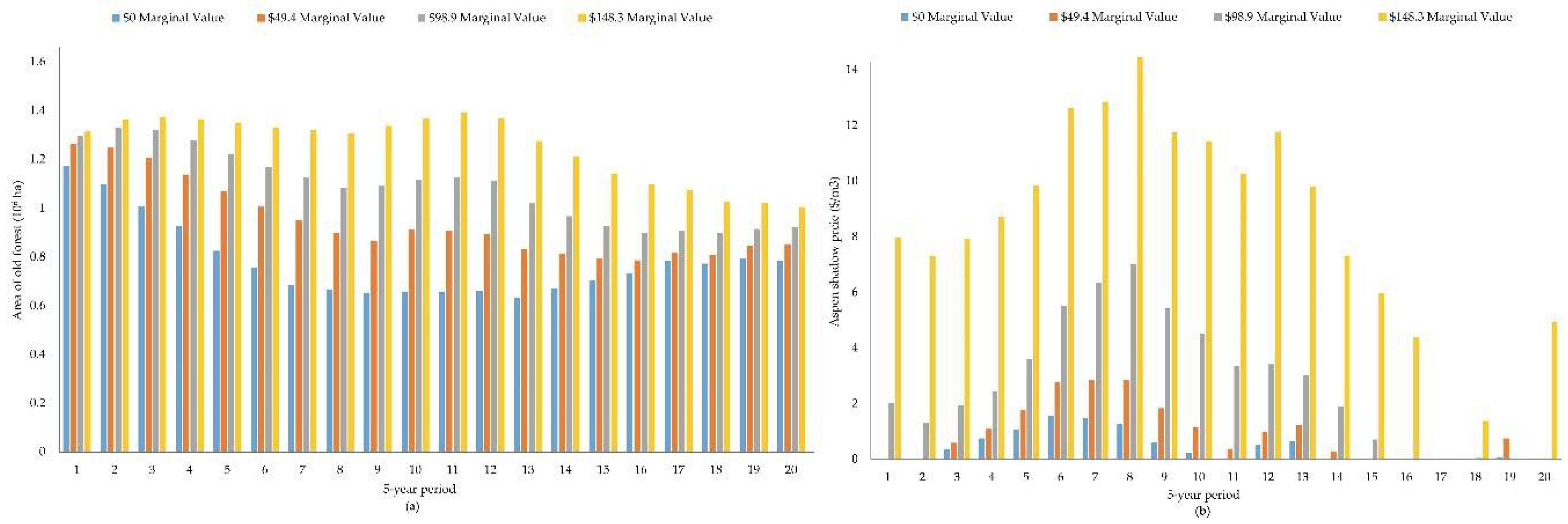
In order to better comprehend the dynamics of the model in relation to the old forest, we first considered alternatives in which old forest has a constant marginal value per hectare, resulting in a horizontal marginal value function with respect to quantity produced. As a baseline, we assumed that environmental preferences towards old forest were absent, so that old forest was valued at $0/ha and timber production was the sole valued service from the forest. We also considered three additional alternatives with horizontal demand curves, raising this horizontal demand curve in increments of $20/acre. Translating to metric units resulted in constant annual values of $49.4/ha, $98.8/ha and $148.3/ha. These marginal value curves essentially included the value of old forest in the objective function of the scheduling model, not forcing the production of old forest through any explicit constraints in the model. Comparing model results for these alternatives will add insight about potential gains from explicitly recognizing a constant old forest value in planning.
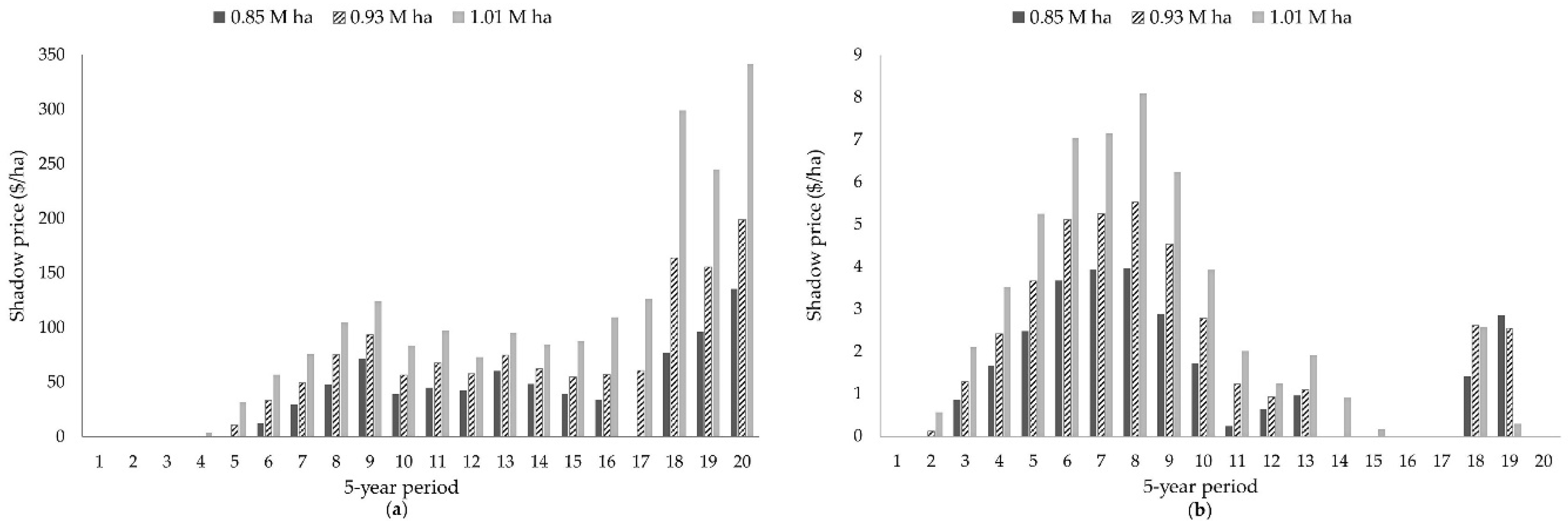
With the intent of assessing the behavior of the model with an approach that forest planners commonly follow to sustain old forest conditions, a second set of alternatives used a fixed target amount of old forest to be achieved at the end of each planning period. These area targets implied vertical demand curves. We considered old forest targets of 0.85 million hectares, 0.93 million hectares, and 1.01 million hectares. These values should not be considered as precise estimates, as they were developed initially as 2.1 million acres, 2.3 million acres, and 2.5 million acres with conversion to hectares, potentially suggesting more precision than intended. Initially, the forest had approximately 1.23 million hectares of old forest; in terms of financial maturity this reflected that much of the forest was initially financially overmature. Modeling results will help add insight regarding whether a wider range of old forest production levels might be realistic.
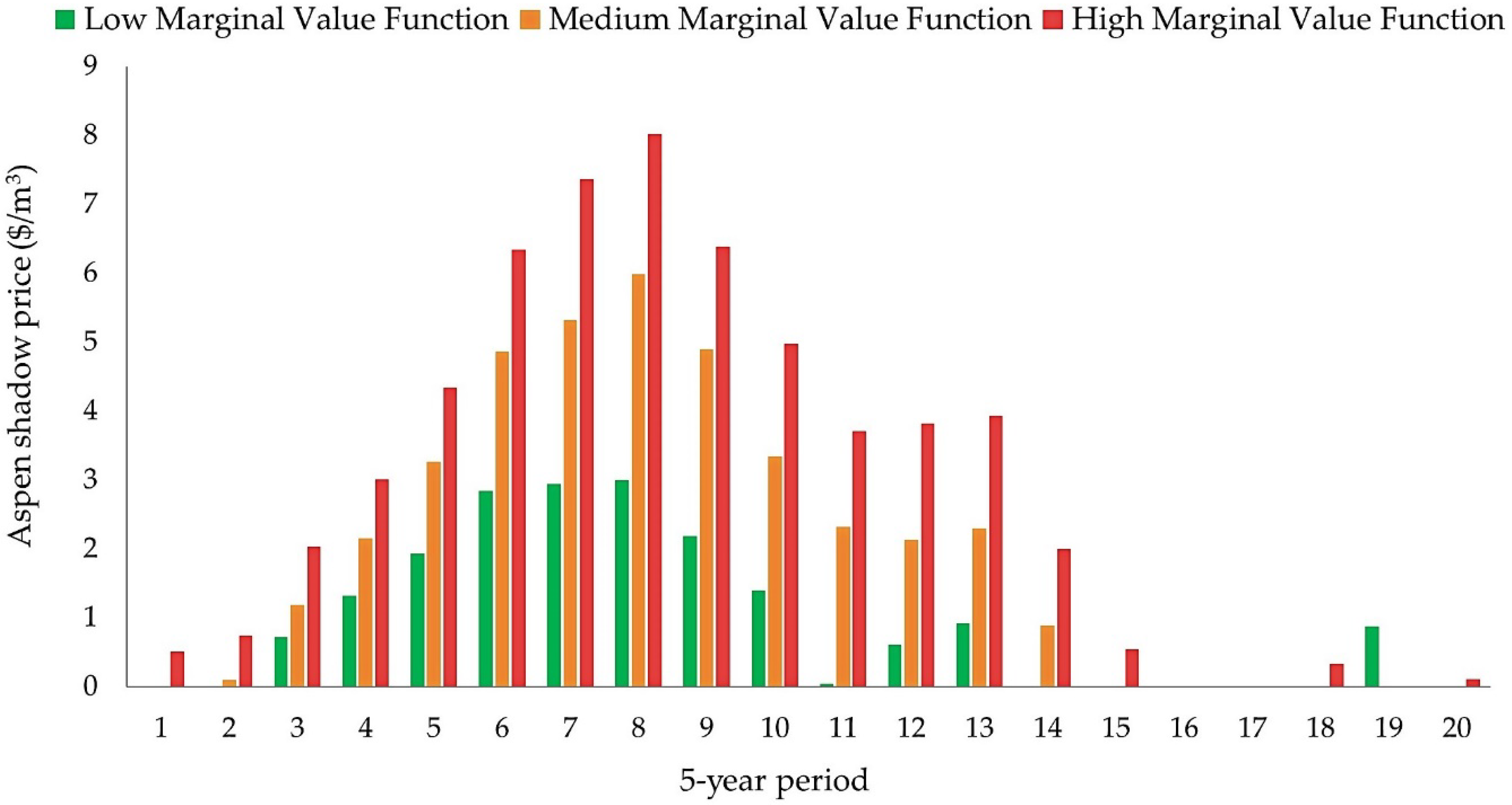
Finally, we defined and explored three additional old forest marginal value curves with a downward slope, to reflect the possibility that stakeholders place higher marginal value on scarce flows of the ecosystem service. To at least some degree, the position and shape of a marginal value function for old forest is a controversial topic, especially when little is known about the potential trade-offs of forest management. Different forest stakeholder groups have quite different values associated with old forest. For example, some in the timber industry would likely argue for keeping marginal values for old forest high for only a short range of old forest production levels and then declining rapidly with increasing quantity. By contrast, some environmental groups might suggest marginal value curves that decline slowly with increasing quantity. To incorporate both views into the study we considered two marginal value functions mimicking these preferences, as well as a third, intermediate option with a constant slope.
Figure 4 shows these three marginal value functions; called high, medium, and low marginal value functions throughout the rest of the paper. Again, these functions relate only to the production of old forest of upland hardwoods for our study area.
The decision to leave an individual stand as old forest or to harvest is a marginal one, having only a small effect on overall timber or old forest production. As a result, that decision entails computing the net marginal benefits (marginal benefits minus marginal costs) of leaving a stand as old forest. The net marginal benefits can be thought of the marginal benefits of recreational opportunities, wildlife habitat, or biological diversity, less any direct costs such as recreation upkeep or increased damages from wildfire. Opportunity costs are already explicitly captured when considering harvesting the stand. The exact numeric values and functional forms we used for marginal values were intended only to cover a range of alternatives, and did not reflect our judgment of a ‘true’ social marginal value curve. All the marginal value functions were assumed to be for the aggregated value of the total old forest and were assumed to be the same for each planning period. Values were in terms of forest condition at the end of each planning period, and were expressed here in annual terms, representing a value that can be added (or credited) as a series of benefits over time for valuing specific stand-level management options. These marginal values varied by periods, since the total area of old forest changes over time.
2.4. Additional Considerations for Northern Minnesota Applications
Overall, our intent was to keep the model simple enough to be useful, yet realistic and aligned to the current forest situation in Minnesota. There is a strong interest in the potential future growth of the forest industry in Minnesota, and all of our scenarios considered some potential expansion of the forest industry in Minnesota. For the first 5-year planning period harvest, levels were constrained to be between 13.77 million m3 and 15.22 million m3. For period two and all periods beyond, statewide harvest levels were constrained to be between 14.5 million m3 and 16.31 million m3. The model recognized premiums for timber by species and product class with the highest prices for red pine sawlogs. Timber prices were delivered prices to the market, including harvest and transport costs.
Aspen harvest levels in Minnesota are of particular interest, because of interest for potential mill expansions and because aspen harvest levels, at least in a long-term perspective, are likely currently near their long-term sustainable level. Also, because of aspen’s general short-lived nature, much of the aspen forest cover type is currently at a stand age where merchantable stand volume is declining and these stands are succeeding to other forest cover types. Current aspen age-class distributions also vary substantially by forest ownership group. The volume of aspen includes the following species: trembling aspen (Populus tremuloides Michx.), bigtooth aspen (Populus grandidentata Michx.), and balsam poplar (Populus balsamifera L.). Recognizing the importance of aspen harvest levels, we considered three alternatives that differ in the assumed volume of aspen harvested per year, while the constraints on the statewide harvest levels are the same for these three alternatives. These alternatives were: (1) the first alternative that forced aspen harvest levels to be at least 5.43 million m3 per year throughout the planning horizon. This was an approximate estimate of the current aspen harvest volume of recent years in Minnesota; (2) a second alternative to assess the behavior of harvest flows under a relatively small mill expansion alternative that increased aspen harvest levels by 200,000 cords annually to a constant level of 6.16 million m3 throughout the horizon planning; and (3) the last alternative where we imposed an early departure of aspen volume levels at 6.16 million m3 per year during the first 20 years of the planning horizon and decreasing those levels to 5.8 million m3 after that, remaining at that 5.8 million m3 level throughout the rest of the 100-year planning horizon. This third “aspen demand” alternative addressed the potential for a short-term increase in aspen harvest levels with some decline in aspen levels longer-term, potentially reflecting shifts in timber demand to more under-utilized species.
Condition sets were defined in Dualplan to help track and constrain production of old forest. The focus was on a condition set that tracked the area of the old forest of upland hardwoods. The area of this condition set included all area in the oak and northern hardwoods forest cover types greater than age 60 years. It also included percentages of the aspen and paper birch (
Betula papyrifera) cover types, with percentages varying by forest cover type, stand age, and ecoregion (
Table 1). Both aspen and paper birch forest cover types are generally short-lived where, if not harvested, a proportion of their area is assumed to have transitioned to a mixed hardwood condition. The transition period is a gradual time period over which the oldest overstory trees die and are replaced by hardwoods assumed to be in the stand. “Age” of the stand is defined in terms of stand age at the start of the planning horizon plus time since the start of the planning horizon, with stand forest cover type not changed explicitly in the specific treatment options used as model input. For example, the 0.3 value for the aspen forest cover type at age 100–105 in the Northeast ecoregion (
Table 1) indicates that 30% of these aspen stands are assumed to meet old forest hardwood requirements. Generally, as reflected in
Table 1, stands in the Northeast portion of the study area transition to hardwoods at a later age. We assume that a higher percentage of the area in the aspen forest cover type produce old forest before transitioning to another forest cover type. However, as also reflected in
Table 1, a lower percentage of the oldest aspen stands in the Northeast transitions to old hardwoods because a substantial proportion of aspen forest cover type in this region will succeed to a mixed conifer condition. In terms of defining the area of old forest hardwoods, the birch forest cover type was not considered to produce old forest until the forest cover type changes, as birch trees are short-lived and generally do not make for good wildlife cavity trees as would aspen trees [
51].
Similar to how some timber products (like pine sawlogs) have premium values, premiums for specific types of old forest conditions were also considered in some scenarios. We also included two additional alternatives to help better understand the potential of shifting old forest production by stand ownership. These alternatives used either high or low premiums based on stand ownership, stand age, and forest cover type (
Table 2). Generally, in terms of ecosystem services, it may be more desirable to have the older hardwood conditions emphasized more on public lands, and potentially more aggregated on the landscape through specific areas like on National Forest system in Minnesota. Premium levels were developed initially in terms of
$/acre/year, with the high precision of the values reported in
Table 2 being somewhat misleading because of conversion to metric units for reporting. Both specific values and premium levels for old forest are certainly difficult to estimate. Our strategy was somewhat like a classic cost-price approach for dealing with price uncertainties where the focus is not on developing and using a specific price estimate, but rather on the sensitivity of results to prices [
52,
53]. Our interest was more focused on shifts in production between ownerships with premiums rather than identifying break-even future prices.
In summary, each scenario corresponded directly with an application of the forest management scheduling model, and each was a unique combination of assumptions concerning three facets described in this methods section: (1) one of ten marginal value functions for old hardwood forest; (2) one of three assumed plausible demand levels for aspen timber volumes over time; and (3) one of three premium levels reflecting relative value differences between the types of old forest produced. For all the scenarios modeled, we used a 100-year horizon planning divided into 20 5-year periods. To calculate the net present value of all stand-level management options, a 4% annual discount rate was used for all scenarios.
4. Discussion
Like the information summarized in
Figure 1, the forest management situation in Minnesota is complex. Management choices are clearly impacting the ecosystem services provided. Structuring a model to address such complexities is clearly a challenge. Here, we discuss briefly a few insights from our experiential learning associated with this study that may be helpful for studies elsewhere.
4.1. Benefits of Using Downward-Sloping Marginal Value Curves
Modeling results for our scenarios suggested the limitations of using constant prices or constant targets for ecosystem services. Initial age-class distributions for the forest are imbalanced, and extremely so for some forest cover types. Our results showed that with constant marginal values assumed for old forest, substantial fluctuations occur in the old forest output levels over time, with levels declining more in later periods for the values we considered. In contrast, when setting old forest targets constant over time, targets were achieved at low-cost short term with substantially higher marginal costs in later periods. Downward-sloping marginal revenue curves fit well with basic concepts of scarcity, reflecting higher marginal values when resources are scarcer. Such an approach also helped overcome problems with setting infeasible or unrealistic old forest targets. With these downward-sloping target levels, targets can vary periodically on their associated marginal cost. In simple terms, users have opportunity to define targets based on associated costs at the margin. Often in forest planning, it is important to consider targets for management, yet such targets are difficult to set until more is learned through analysis of production possibilities. Also, in forestry, these possibilities substantially change over time as forest conditions change. Also, the temporal scale is important, as old-forest values are typically time series of benefits at the stand level, with it generally important to plan ahead.
4.2. Importance of Forest-Level Analysis Across Forest Cover Types
Our applications also demonstrate some of the difficulties and over-simplifications of addressing forest cover types separately. The composition of individual stands changes with succession, resulting in a shift or change in the forest cover type. This is especially true for short-lived species like aspen. Unless natural disturbance rates are high, relatively new forest reserve areas will take time to develop into a more steady-state old forest condition, and even then, forest-level conditions will vary substantially over time unless we are dealing with vary large landscapes. Some forest cover types, like aspen in Minnesota, are critical for sustaining local timber economies. Other forest types, like northern hardwood, are more complex in ecological structure and may be better suited for producing a mix of economic and ecological benefits, especially if uneven-aged management can be financially viable. Our results also demonstrate that the general wood supply situation in Minnesota, in terms of its ability to support additional economic development, is especially sensitive to specific tree species needed for development opportunities in question. Although aspen is of major value to the existing forest industry in Minnesota, opportunities for additional expansions based primarily on aspen would likely cause substantial timber supply challenges to existing forest industry. The situation is quite different for other species and forest cover types. Generally, most of Minnesota’s forest cover types are currently financially overmature, as is consistently shown in all our scenarios with the forest-level “even flow” harvest volume constraints at their upper bounds in early periods and at lower bounds in later periods. Even without considering climate change impacts, with Minnesota currently having a preponderance of older stands that are currently growing slowly, it does not seem all that surprising that forest insect and disease outbreaks are increasing and could be quite devastating, especially for some forest cover types.
4.3. Benefits of Analysis across Ownerships
With Minnesota having a mosaic of ownerships, there is clear value for large ownerships to better understand their management situation in a forest-wide landscape context. This was one clear need identified by a major recent analysis of Minnesota DNR timber harvest levels [
54]. Additionally, for economic development opportunities, one cannot fully understand the supply situation if it is not analyzed over a broad landscape that recognizes the details of market demands. Another consideration is the production of fewer timber products, but with timber products being more valuable. Emphasizing more the value than the quantity of timber produced, will almost certainly integrate better with additional objectives associated with ecological services.
It is also important to recognize that our analyses have used optimization modeling, including nonmarket objectives. Our intent is not to show predictive results, but to help identify needs and understand trade-offs. Certainly, one cannot control private landowner behavior directly through broad landscape-level forest management scheduling. For example, our results certainly suggest that harvesting more of the older aspen on private lands in the short-term, as otherwise substantial volumes will be lost from the market for what appears a relatively tight timber supply situation for aspen that may continue for 40 years or more.
4.4. Additional Details, Data Needs and Further Analysis
Results are certainly sensitive to assumptions about private landowners. Detailed data on the behavior of private landowners in Minnesota and elsewhere is limited at best. However, the fact that a financially overmature aspen stand is even present on the landscape suggests that this landowner is unlikely to harvest this stand in the near future—many of these landowners have been approached by wood procurement foresters in the recent past and have declined harvest offers. Modeling results are also certainly sensitive to basic data involving growth and yield data, especially for the aspen forest cover type. The recent statewide Minnesota DNR study highlights this need [
54]. Specifically, their study points out the sensitivity of their results to the aspen growth and yield data used. Aspen timber prices are also very sensitive to seasonal limitations on harvests, which we did not address in our scenarios. Limited information is also currently available on harvest costs. And although FIA inventory data is relatively current, future work might look at potentials of integrating inventories from major landowners into a landscape analysis. This would help allow for more site-specific and spatial detail, which are important for ecosystem services. Also, how short-lived cover types will change forest cover types over time is certainly not clear. In Minnesota and elsewhere, detailed analyses for forest planning helps to identify important information needs for forest management.


