The Short-Term Effects of Experimental Forestry Treatments on Site Conditions in an Oak–Hornbeam Forest
by
 ,
,
Bence Kovács
1,2,3,* ,
,
Flóra Tinya
1,
Erika Guba
1,
Csaba Németh
2,
Vivien Sass
4,
András Bidló
4 and
Péter Ódor
1,2 1
MTA Centre for Ecological Research, Institute of Ecology and Botany, Alkotmány út 2-4, H-2163 Vácrátót, Hungary
2
MTA Centre for Ecological Research, GINOP Sustainable Ecosystems Research Group, Klebelsberg Kuno utca 3, H-8237 Tihany, Hungary
3
Department of Plant Systematics, Ecology and Theoretical Biology, Eötvös Loránd University, Pázmány Péter Sétány 1/C, H-1117 Budapest, Hungary
4
Institute of Environmental and Earth Sciences, University of Sopron, Bajcsy-Zsilinszky utca 4, H-9400 Sopron, Hungary
*
Author to whom correspondence should be addressed.
Forests 2018, 9(7), 406; https://doi.org/10.3390/f9070406
Submission received: 4 June 2018
/
Revised: 2 July 2018
/
Accepted: 3 July 2018
/
Published: 5 July 2018
(This article belongs to the Section Forest Ecology and Management)
Abstract
:Forest management alters forest site; however, information is still limited about how different silvicultural treatments modify abiotic conditions. We compared the effects of four treatments from three different forestry systems on forest microclimate, litter, and soil conditions. The clear-cutting, retention tree group, preparation cutting, and gap-cutting treatments were experimentally established in a European oak-dominated forest, following a complete block design with six replicates. In this study, we show the results of the quantitative analyses of 21 variables, one year after the interventions. Strong treatment effects were observed for the microclimate and litter variables, whereas the soil characteristics remained similar. The increase in light was the highest in the clear-cuts with intermediate effects in the gap-cuts. The means and variances of the air and soil temperature as well as the vapor pressure deficit were the highest for the clear-cutting treatment. An increase in soil moisture, litter pH, and litter moisture was significant in the gap-cuts and, to a smaller extent, in the clear-cuts. The soil pH increased in the retention tree groups. Microclimatic differences between the treatments were the largest during the summer, which demonstrates the buffering effect of the canopy. Our study confirms that less intensive and more spatially heterogeneous silvicultural treatments (e.g., gap-cutting) preserve a stable below-canopy microclimate more effectively. These results can support and might be useful for both forest management and conservation planning.
1. Introduction
Forest management induces substantial alterations in environmental conditions that fundamentally influence the ecosystem’s structure and functions [1,2]. These strongly impact the long-term survival, regeneration, and diversity of forest-dwelling organism groups [3,4]. Silvicultural treatments can directly generate changes in forest biodiversity by deteriorating communities associated with individual trees and tree-related microhabitats, such as epiphytes [5], deadwood-dependent communities [6], and cavity nesters [7]. Most of the forest-dependent taxa are indirectly influenced by forest management through the alteration of site conditions—microclimate, litter attributes, and soil characteristics—and biogeochemical cycles [8,9,10,11,12]. The microclimate is also a major driver of ecosystem processes such as decomposition, respiration, and nutrient dynamics [13,14]. Studying the effects of different management practices on forest site conditions can support the mitigation of the negative impacts of climate change [15,16], because fine-scale measurements and high-resolution models are necessary to create predictions for the ecological processes or calculate probable species distributions [17,18]. Therefore, for conservation purposes, it is important to investigate how forestry treatments alter forest site conditions through numerous, highly interrelated effects.
Forest stands create a unique, buffered below-canopy microclimate [19,20] compared to open-fields [21] or to plantations [22]. This buffering capacity is mainly determined by the tree species composition, tree species richness, and stand structure, as the foliage of the different vegetation layers absorbs a large proportion of incoming solar energy and reduces the loss of longwave radiation from the surface [21,23,24,25]. The soil and litter characteristics are also influential [26,27]. As a result of these effects, forest microclimates can be characterized by lower diurnal and seasonal magnitudes, in case of several microclimatic variables [19,26]. Similarly, the litter layer is important for many decomposer groups as a habitat and food resource, as well as for nutrient cycling, smoothing the fluctuations of the physical and chemical properties of the topsoil, and the below-canopy ambient air [9,28].
Alterations of the microclimate, litter, and soil properties, and thus changes in forest communities, are highly dependent on the spatial extent, the spatiotemporal pattern, frequency, and severity of the forest management approaches applied [29,30,31]. Changes in the main structural elements of forests (e.g., canopy closure, horizontal, and vertical foliage distribution) result in considerable alterations in the processes of the soil–vegetation–atmosphere system. This effect is obvious for clear-cuts [32,33,34], but it is also observable in partial cuts like thinning, group selection, or retention tree harvesting [11,35,36,37,38,39].
Even though forest management in the temperate zone is shifting globally from even-aged rotation management systems towards continuous-cover silvicultural approaches that support structural heterogeneity, we have limited information about how the different forestry interventions affect the forest site conditions [31]. Forestry experiments are necessary for the understanding of the complex relationships between different management practices and forest site, regeneration, and biodiversity characteristics. However, as Bernes et al. pointed out, there is a knowledge gap concerning the possible multipurpose forest management alternatives in Central European deciduous forests [40]. There are studies that examine the effects of multiple treatment levels within a particular silvicultural system on microclimate, such as different artificial gap sizes and shapes [35,41], various combinations of retention levels and spatial configurations [36], thinning intensities and patterns [42,43], and fuel-reduction oriented treatments [44]. Similarly, changes in soil characteristics and biochemical processes have been shown in lower intensity harvest types [13,37,39,45]. Most of the studies dealing with the interactions between harvesting and forest site conditions concentrate on one selected forestry system. Two or more silvicultural strategies have rarely been applied within one experimental design (but see, for example, [11] or [14]).
The ‘Pilis Experiment’ was implemented to compare the effects of different treatment types on site conditions, regeneration and biodiversity. All of the alternative silvicultural systems applicable to European forests were included (clear-cutting, shelterwood system and continuous-cover forestry with gap-cutting; [46]). All of the established treatment types—clear-cutting, gap-cutting, preparation cutting, and retention tree group—are common practice in the temperate regions of Europe. To model large clear-felled areas (usually created by the clear-cutting system or shelterwood system, in the course of the final cutting), clear-cutting was applied. This is the most extreme yet widespread silvicultural treatment type, applied in even-aged rotation forestry. The study of retention tree groups inside clear-cuts is particularly interesting. Recently, the application retained groups of individuals has been spreading, as they mitigate the impacts of clear-cutting, an important goal of nature conservation in forests. The shelterwood system is represented here in the form of preparation cutting, which is the first step towards the final cutting. Moreover, it is a form of partial cutting, comparable to thinning or dispersed green tree retention. In Central Europe, continuous cover forestry is typically practiced via artificial gaps or group selection, therefore, gap-cutting was also part of our study. Our open-field, multi-taxa experiment was established in 2014 [47]. As a target habitat type, sessile oak (Quercus petraea Matt. [Liebl.]) and hornbeam (Carpinus betulus L.) forests were chosen, which represent a deciduous woodland habitat type widespread in the Pannon Ecoregion [48] and generally in Central Europe [49]. This is one of the focal indigenous forest types for timber harvesting in this region, because of the high-quality timber of sessile oak [50]. Here, we focus on the effects of the experimental treatments on site conditions during the first post-harvest period. Our objectives are to quantify the differences induced by the applied management treatments (clear-cutting, gap-cutting, preparation cutting, and retention tree group) (1) on the mean and variability of microclimate, soil, and litter variables during the growing season; (2) on the temporal pattern of site condition variables through a growing season; and (3) on the diurnal patterns of selected microclimate variables.
We hypothesized that the microclimate responds to the treatments immediately, whereas changes in the litter and soil variables were expected to be delayed. Clear-cutting affects the forest site most strongly. For the majority of our variables, we supposed that the retention tree group mitigates the harsh environmental conditions generated by clear-cutting. We presumed that gap-cutting and preparation cutting cause intermediate changes in the forest site conditions. We also presumed that differences from the control are more expressed in the summer, at the peak of the growing season, when the canopy closure of the control is the highest. This will also be discernible in the form of larger disjunctions in the diurnal cycles of the microclimate.
2. Materials and Methods
2.1. Study Area
The study was conducted in the Pilis Mountains, north-eastern ridge of the Transdanubian Range, Hungary (47°40′ N, 18°54′ E; Figure 1a). Plots are situated on a horst ridge (370–470 m above sea level) on moderate (7.0–10.6°), north-facing slopes. The average annual mean temperature is 9.0–9.5 °C (16.0–17.0 °C during the growing season), with a mean annual precipitation of 650 mm [51].
The bedrock consists of Dachsteinian limestone and Lattorfian sandstone with loess [51]. According to the soil profiles established in the study site, the soil depth varies along a slight topographic gradient (Supplementary Materials 1), deep (250 cm) at the lower elevations and shallow (70 cm) nearer the ridge. In the lower elevation parts of the site, the soil type is brown forest soil with clay illuviation (Luvisol), while in the upper parts it is Rendzic Leptosol [52]. The soils are slightly acidic (pH of the 0–20 cm layer is 4.6 ± 0.2). The physical and chemical characteristics of the upper 50 cm of soil are similar in the whole area, independent of soil depth (Supplementary Materials 1). The variety of soil types did not cause a discernible variability in the woody vegetation (Table 1).
The study site was established in an approximately 40 ha sized homogeneous unit, in a managed, two-layered sessile oak–hornbeam forest stand (Natura 2000 code: 91G0 [53]). The stand is even-aged (80 years old) and has a relatively uniform structure (Table 1) and species composition, because of the applied shelterwood silvicultural system. The upper canopy layer (average height 21 m, mean diameter at breast height (DBH) 27.6 cm) is dominated by sessile oak, while the second most abundant tree species, hornbeam, forms a subcanopy layer with an average height of 11 m and a mean DBH of 11.6 cm (Table 1 and Figure S2.2). Other woody species are rare, and individuals of Fraxinus ornus L., Fagus sylvatica L., Quercus cerris L., and Cerasus avium L. were recorded in the tree layer as admixing tree species. Before the experimental treatments, the mean basal area (BA) of the upper layer was 29.4 (±4.3) m2 ha−1 and 8.8 (±2.6) m2 ha−1 in the case of the secondary canopy layer, respectively (Table 1). The canopy closure was rather homogenous, varying between 81% and 94%. The shrub layer was scarce and mainly consisted of the regeneration of hornbeam and Fraxinus ornus L. with a lower cover of shrub species (e.g., Crataegus monogyna Jacq., Cornus mas L., Ligustrum vulgare L., and Euonymus verrucosus Scop.). The understory layer was formed by general and mesic forest species. Dominant species were Carex pilosa Scop., Melica uniflora Retz., Cardamine bulbifera L., Galium odoratum (L.) Scop., and Galium schultesii Vest. Before the treatments (in 2014), the herb layer cover was approximately 40%.
2.2. Study Design
Five treatment types (Figure S2.1) were implemented in a randomized complete block design in six replicates (hereafter blocks, Figure 1b,c, and Table 1):
- Control (C): The original stand characteristics remained unaltered.
- Clear-cutting (CC): Approximately 0.5 ha sized circular clear-cuts were formed, surrounded by a closed-canopy stand. The area of the treatment was designated as the area surrounded by the trunks of the peripheral dominant forest trees, the applied diameter was 80 m. Within the clear-cuts, every tree individual (DBH ≥5 cm and/or height ≥2 m) was cut.
- Gap-cutting (G): Circular artificial gaps were established in the closed stand by the elimination of all of the tree individuals within a diameter of 20 m (~0.03 ha). Gap size was defined as expanded gaps [54] (i.e., by measuring the base of surrounding canopy trees). The chosen 1:1 gap diameter/intact canopy height ratio is widely used in Central Europe for transition system applying gap-cutting, and it also fits well with the records of gap area in oak forests [55,56].
- Preparation cutting (P): Uniform partial cutting was applied within a circle with a diameter of 80 m, and 30% of the initial total basal area of the upper canopy layer was cut in a spatially even arrangement. Furthermore, the complete subcanopy- and shrub-layer were also removed.
- Retention tree group (R): All of the tree and shrub individuals were retained within a 0.03 ha sized circular plot (diameter = 20 m) in the clear-cuts, which resulted a small patch of the remained stand with approximately 8–12 trees of the former upper layer.
In accordance with the operative forestry law, individual clear-cuts in the submontane regions of Hungary are less than 5 ha [57]. The created clear-cuts are substantially smaller than it is typical in Hungary or in the temperate deciduous forests in Europe (3–10 ha). Therefore, changes in the site conditions resulting from this treatment may be less pronounced. In our experiment, neither the plots representing clear-cutting, nor the retention tree groups were placed in the center of the clear-cuts (Figure S2.2). These plots were shifted to the 1:3 intersections along the east–west axis, because we intended to minimize the bias caused by the shading of the remained trees of retention tree groups in the clear-cutting plots.
All of the treatments were carried out in the winter of 2014–2015. In the center of the treatments, a 6 m × 6 m fenced area (hereafter plot) was established to exclude the effects of the large-bodied game species.
2.3. Data Collection
Microclimate variables (total photosynthetic active radiation, air temperature, relative humidity, soil temperature, and soil moisture) were recorded every month of the growing season (March–October) of 2015 (directly after the implementation of the treatments). The litter and soil variables (litter mass, litter pH, litter moisture content, soil pH, hygroscopicity, and nutrient content) were measured in April and October of 2015.
Systematic microclimate measurements were taken in the center of each plot. Temporally synchronized data collection was carried out using 4-channeled Onset ‘HOBO H021-002′ data loggers (Onset Computer Corporation, Bourne, MA, USA) mounted on wooden poles (Figure S2.3). Every month of the growing season (March–October), 72 h logging periods were applied with 10 min logging intervals. Photosynthetically active radiation (PAR, λ = 400–700 nm; μE m−2 s−1) was measured at 150 cm above ground level, using Onset ‘S-LIA-M003′ quantum sensors (Onset Computer Corporation, Bourne, MA, USA). Air temperature (Tair; °C) and relative humidity (RH, %) data were collected 130 cm above ground level with Onset ‘S-THB-M002′ (Onset Computer Corporation, Bourne, MA, USA) combined T/RH sensors (Onset Computer Corporation, Bourne, MA, USA) housed in standard radiation shields to avoid direct sunlight. The soil temperature (Tsoil; °C) was measured with ‘S-TMB-M002′ 12-Bit temperature sensors (Onset Computer Corporation, Bourne, MA, USA) by Onset placed 2 cm below ground. Soil water content (SWC; m3/m3) data were collected using Onset ‘S-SMD-M005′ soil moisture sensors (Onset Computer Corporation, Bourne, MA, USA) buried 20 cm below ground level to measure the average soil moisture at 10–20 cm soil depth. Air temperature and relative humidity data were used to calculate vapor pressure deficit (VPD; kPa) values at every logged occasion, following the protocol of Allen et al. [58], VPD = (0.6108){exp[17.27·Tair/(237.3 + Tair)]}·(1 − RH/100). The reason for using VPD as a dependent variable is that it can give a direct indication of the atmospheric moisture conditions independently of the actual temperature. Therefore, it is a good standalone indicator of the atmospheric factors influencing evaporation; VPD describes the actual drying capacity of air (i.e., the higher the VPD is, the more intensive is the evaporation) [59]. Additionally, the relative diffuse light (DIFN; %) was measured using an LAI-2000 Plant Canopy Analyzer (LI-COR Inc., Lincoln, NE, USA) in the center of each plot at 130 cm above ground level. The measurements were carried out in August at dusk to avoid direct light affecting the sensor. Repeated measurements are not needed with this device [60]. A 270° view restrictor masked the portion of the sky containing the sun and the operator [61]. Reference above-canopy measuring was performed on an adjacent open field.
At each plot, four litter (30 cm × 30 cm area) and topsoil (0–20 cm depth) samples were systematically collected. All of the samples were returned to the laboratory and following the necessary preparation steps, and the litter mass, litter pH, litter moisture content, Kuron’s hygroscopicity (hy), soil organic matter content, and nutrient content were measured. The litter mass was measured after the samples were air-dried to a constant mass. The litter moisture content (%) was calculated as the mass loss of the freshly collected litter samples (i.e., the difference between the fresh and dried litter).
The litter and soil pH were potentiometrically measured using the supernatant suspension of air-dried and sieved (<2 mm) samples and 25 mL of distilled water, and the applied mass was 5 g for litter and 10 g for soil samples, respectively [62]. Kuron’s method was applied for gauging the hygrscopicity (hy) of air-dried soils [63], with a 50% (v/v) H2SO4 solution and 35.2% RH, according to [62]. The chemical compounds were evaluated on the composite samples of the 1:1 mixture of the four sieved (<0.5 mm) subsamples per plot. The total soil carbon and nitrogen content were determined by dry combustion method using the Elementar vario MAX CNS-analyzer (Elementar Analysesysteme, Langenselbold, Germany), applying the International Organization for Standards (ISO) standards [64,65], as follows: the soil samples were weighed between 80 and 100 g, and a tungsten oxide catalyst was added. The applied combustion temperature was 1140 °C. Plant available phosphorus and potassium were determined by the ammonium lactate (AL) solution method (0.1 M NH4 − lactate + 0.4 M HOAc, adjusted to pH 3.75), developed by Egnér et al. (1960, cf. [66]), according to the operative Hungarian standards [67]. The concentration of AL-soluble phosphorus (PAL) was measured colorimetrically, the concentration of AL-soluble potassium (KAL) was quantified by flame photometry.
All of the studied variables were also recorded in 2014 (pre-treatment conditions), applying the same methodology. The pre-treatment conditions of the plots selected for the different treatment levels were similar in 2014 (Table S3.1).
2.4. Data Analysis
The microclimate data were initially screened and the obvious errors caused by technical failures (indicated by, for example, unrealistic data or large spikes in variables) were replaced by missing values. The manually corrected data were imported into the database built in SpatiaLite 4.3.0a [68]. The observations were split into 24 h datasets. The differences from the values collected at the control were calculated for every recording (control values were subtracted from the treatment values of the block), and then the daily mean and interquartile range (IQR) of these difference values were computed. To measure the direct effects of the silvicultural treatments on the site condition variables, these relative data were used to avoid the effects of actual weather conditions and local differences between the blocks. For the analyses, one randomly chosen 24 h microclimate dataset was used every month. Daily IQR of the soil water content (SWC) was excluded from the analysis, because soil moisture is a rather stationary variable. For the relative humidity (RH) and vapor pressure deficit (VPD), as a result of numerous missing data, the subset of October was excluded.
The temporal patterns of the measured variables were investigated using two different temporal resolutions, according to the distinct methods for soil chemical variables and litter parameters, the seasons were compared (spring vs. autumn); while in the case of the microclimate variables, we used months as factor levels.
To explore the effect of the treatments and time on the measured site condition variables, linear mixed effects models (random intercept models) with a Gaussian error structure were used [69]. Where necessary, the data were transformed to achieve the normality of the model residuals. The effects of the different treatment levels across (1) the whole growing season and (2) over the applied temporal resolution (month or season) were tested by the same modeling framework, as follows: the treatment, time, and their interaction were used as fixed factors, while the block was specified as a random factor. The models’ goodness-of-fit values were measured by a likelihood-ratio test-based coefficient of determination (R2LR; [70]). The differences between the treatment levels were evaluated using the Tukey procedure (alpha = 0.05) for all of the pairwise comparisons. Multiple comparisons were applied to analyze the differences among the treatments throughout the growing season, based on the group means (‘glht’ function of ‘multcomp’ package; [71]), within the time levels on the least-squares means (‘lsmeans’ function of ‘lsmeans’ package; [72]). The significance of the differences between the control and the other treatment levels was tested using linear mixed effects models, without intercept [73].
The diurnal patterns of the selected microclimate variables were shown using the original values (raw data). These were analyzed qualitatively, without any statistical test, applying the standard locally weighted scatterplot smoothing (LOWESS) analyses with 95% confidence intervals. The datasets were pooled into two groups, the peak of the growing season (i.e., June, July, and August) and the transitional period (March, April, September, and October) with lower canopy closure. Smoothing procedures were applied on 24 h datasets with six replicates for each treatment level.
The data analyses were performed using R version 3.4.1 [74]. inear mixed effects models were conducted by R package ‘nlme’ [75], and multiple comparisons were appraised using the ‘multcomp’ [71] and ‘lsmeans’ [72] packages. The determination coefficients of the models were calculated using the ‘rsquaredLR’ function of the ‘MuMIn’ package [70]. For graphing, the modified script of the ‘errorbars’ function was used [76].
3. Results
3.1. The Effects of Experimental Treatments on Site Condition Variables
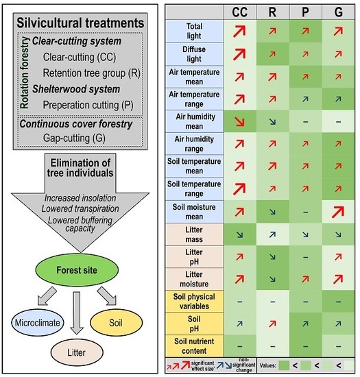
According to the performed linear mixed effects models (see Supplementary Materials 4 for details), we found that the experimental treatments affected microclimate and litter variables more, while the soil chemical characteristics did not differ significantly among treatment types—except for topsoil acidity (Table 2 and Figure 2).
The mean (Figure 2a) and the IQR (Figure 2b) of photosynthetic active radiation (dPAR), as well as the mean of relative diffuse light (dDIFN, Figure 2c) were substantially higher in all of the treatments than in the controls. The largest values were detected in the clear-cuts, and the increment was also considerable in the gap-cuts. The light conditions were similar in the preparation cuts and the retention tree groups, but the dDIFN was lower in the retention tree groups. The mean and interquartile range of the air temperature (dTair) departed significantly from the control in all of the treatments (Figure 2d,e). In the retention tree groups and clear-cuts, the mean of the dTair was significantly higher than in the other two treatments (Figure 2d). The dTair was buffered the most in the preparation cuts, but the mean of dTair was not different from that in the gap-cuts. Both the mean and the standard deviation of the IQR were the highest in the clear-cuts (Figure 2e). The lowest IQR was measured in the gap-cuts, while in the other treatments, the IQR was intermediate. The mean of relative humidity (dRH) was the lowest in the clear-cuts and in the retention tree groups (Figure 2f). In the preparation cuts and gap-cuts, the humidity remained similar to the control; furthermore, these treatments did not differ from each other. It is noticeable that the IQR of the dRH was the lowest in the gap-cuts and the highest in the clear-cuts, however, in all of the treatments, the IQRs of the dRH were departed from the control (Figure 2g). The mean and IQR of the vapor pressure deficit (dVPD) showed the same pattern as dTair, because of the high contribution of temperature to this variable, and all of the treatments also differed significantly from the control (Figure 2h and Figure 2i, respectively). The mean and IQR of the soil temperature (dTsoil) differed significantly in every treatment from the control (Figure 2j and Figure 2k, respectively). The clear-cutting created soil thermal conditions that divaricated the most from those in the closed stand; both the mean and IQR of the dTsoil were the highest there. In the retention tree groups, the mean of the dTsoil did not differ significantly from that of the clear-cuts, but the IQR was significantly lower there. The coolest soil environment with the lowest IQR was detected in the gap-cuts. The soil moisture (dSWC) differed significantly in the clear-cuts and even more in the gap-cuts from that in the controls (Figure 2l). The highest dSWC was measured in the gap-cuts, the increase was smaller in the clear-cuts, while a slight decrease was detected in the preparation cuts and in the retention tree groups, and the latter was the driest treatment.
The litter variables showed a strong response to the treatments (Table 2). In the first year, there was no significant response in the litter mass, however, it showed an increasing trend from the clear-cutting to the retention tree group (Figure 2m). In the clear-cuts and in the gap-cuts, the litter pH departed significantly from that in the controls, and the litter were more neutral in these two treatments than in the preparation cuts and in the retention tree groups (Figure 2n). The litter moisture followed the sequence of dSWC. The forest floor was the driest in the retention tree group, but it was not significantly different from that in the controls, and the litter moisture was significantly higher in the other three treatments—the highest values were measured in the gap-cuts (Figure 2o). Among the soil variables, only the soil pH showed a significant treatment effect, the topsoil was less acidic in the preparation cuts than in the other treatments and it was the only treatment level where the soil pH differed from the control (Table 2, Figure 2p).
3.2. Temporal Differences among Treatments through the Growing Season
Besides the study of the treatment effects, the temporal differences during a growing season were also analyzed (Table 2). Except for the light and soil moisture variables, the effect of time was similar or stronger than that of treatments. For the litter mass and potassium content, only the effect of time was significant.
The largest differences in the microclimate variables were detectable in summer (Figure 3). dPAR was the highest in the clear-cuts in almost every month, but the differences were the highest in full-leaved months—from May to August (Figure 3a). The dVPD values were highly divergent among the treatment levels during summer, the drying capacity of air was significantly higher in the clear-cuts and in the retention tree groups, while the dVPD did not depart substantially from the control in the case of the two other treatment types (Figure 3b). dTsoil was the largest in the clear-cuts with the highest variance during the summer (Figure 3c); the differences between the treatment levels accelerated as the canopy closure increased, but gap-cutting and preparation cutting created similar conditions to the control during the whole growing season. The retention tree group could partly buffer the dTsoil. As the first frosts appeared (in October), the dTsoil differed significantly from the other treatments in the clear-cuts (i.e., the soil was the coldest there). The dSWC increment in the gap-cuts was detectable through the whole measurement period, and it increased during summer (Figure 3d). It was also relatively high in the clear-cuts, but the difference was less pronounced than that in the gap-cuts. A moderate soil desiccation was detected in the retention tree groups from June to September.
The litter mass decreased from spring to autumn in the treatments, except for the retention tree group (Figure 4a). The litter pH increased in the gap-cuts and in the clear-cuts in autumn, while in the preparation cuts and in the retention tree groups, it stayed close to the values that had been measured in the uncut controls (Figure 4b). The litter moisture content increased marginally in the preparation cuts and more markedly in the clear-cuts, as well as in the gap-cuts, as compared to the degree of humidity measured in spring (Figure 4c). We found that the effect of time was significant for pH and KAL-concentration (Table 2). The soil pH was lower in spring than in autumn, and in both periods, it was higher in the retention tree groups than in the other treatments (Figure 4d).
3.3. Diurnal Pattern of Microclimate Variables among the Treatments
When we analyzed the 24-h datasets, a clear diurnal pattern could be detected for the different microclimate variables with large variability between the treatments in summer (Figure 5). Contrarily, when the pooled early spring and autumn subsets were analyzed, differences were much smaller and the pattern was not as obvious.
The PAR differed considerably between the treatments in summer. It frequently exceeded 2000 μE m−2 s−1 in the clear-cuts, while in the second brightest plots, in the gap-cuts, the maximum values were under 1930 μE m −2 s−1. There was a detectable lag of the maximum values as follows: in the clear-cuts, it appeared at 12:00–12:20 Coordinated Universal Time (UTC); at around 12:30–12:40 UTC in the gap-cuts; and at 13:10–13:20 UTC in the preparation cuts. In the retention tree groups, the maximum values occurred between 9:00 and 10:30 UTC. This was followed by a decrease in radiation because of the shading effect of the canopy patch. The pattern of irradiance among the treatments was also detectable in the case of VPD and Tsoil, for instance, in the morning, the retention tree group was the warmest and driest treatment. In the clear-cuts, it sometimes reached 38.8 °C in summer, but even in the retention tree groups, its maximum was 31.3 °C. In the gap-cuts, the moist soil (dSWC) was the highest (Figure 2l), resulting in a distinct peak in VPD, which was followed by a quick decrease; and the Tsoil was lower, despite the high PAR. The clear-cuts cooled down the most in the summer, between 2:00 and 7:30 am, and especially in the transitional period. In the transition period, the amplitudes of the diurnal cycles were substantially smaller. Furthermore, the microclimate within the applied treatments did not differ as much as during the peak of the growing season as it did during the other seasons.
4. Discussion
4.1. Rapid Changes in Microclimate and Litter Variables, but Not in Soil Properties
In general, and in accordance with our expectations, the microclimate variables showed strong short-term deviations among the different silvicultural treatments. Interestingly, the litter characteristics also changed in the first growing season. As presumed, we could not demonstrate significant changes for most of the investigated soil variables (physical or chemical). Two different, but highly interrelated processes can be highlighted in the context of microclimate alteration by forest management, radiation balance and evapotranspiration. The forest canopy plays an important role in both of the mechanisms. The maintenance of the buffered microclimate in the below-canopy space of the closed forest stands is based on the shielding effect, namely, through the (partial) shading and the absorption of the foliage, there is significantly less net radiation to heat the forest floor. Moreover, the canopy insulates the understory environment by reducing the longwave radiative loss [19,26,43]. Furthermore, as demonstrated by Bristow and Campbell [77], there is a strong correlation between solar irradiance and transferred heat-related variables of the ambient air, such as air temperature, relative humidity, and vapor pressure deficit. This may explain why, in the harvested sites, we measured a generally higher and temporally more variable irradiance, temperature, and vapor pressure deficit, and a lower, but also more unbalanced air humidity. The changes in the soil moisture following the different treatments are based (1) on the lower rate of interception and evaporation through the canopies or trunks and, consequently, the increased throughfall; and (2) on the lower transpiration rates due to tree removal [32,78,79]. The major effect of these alterations is that the soil water content typically increases in sites where felling was applied on to larger continuous extent (i.e., in gap-cuts and clear-cuts).
4.1.1. Light Variables
As the applied treatments mainly modified the canopy closure of the stand, the (1) total and diffuse light departed from the control in every treatment because of the harvest-induced canopy modifications, and (2) the light variables had the strongest response to the treatments. Our findings are congruent with previous research, showing that the increment in irradiance and its variability highly correlate with the increase of canopy openings and the leaf area index [19,22,33,35]. Therefore, solar radiation is higher and temporally more variable in the clear-cuts than that in the forest edges [80], in the stands harvested by various types of green tree retention schemes [36] or in the management practices related to the uneven-aged systems [8].
The canopy gaps also create a more illuminated environment [81,82,83], although the irradiance was significantly lower than that detected in the clear-cuts, because of the smaller sky view factor [35] and consequently, the shading of the surrounding trees [41]. The preparation cuttings and retention tree groups did not show clear differences in the light level and its variance. These treatments engender a similarly brighter environment than the uncut sites [36,84,85].
The spatial arrangement of the trees influenced the direct-diffuse light proportions. In the preparation cuts, the uniform distribution of the trees strongly inhibited the direct irradiation, but less notably the diffuse light. Therefore, interestingly, the amount of the diffuse light is similar to that in the gap-cuts, but the amount of total irradiance is significantly lower [83,86]. The retention tree group—in the first year—was very open to the adjacent clear-cutting and to the lateral irradiance because of the lack of lower branches and the sparse shrub layer. However, we can expect that the illumination in the retention tree groups will decrease and return to the level characteristic in the control, as the natural regeneration (shrubs, sprouts, and juvenile trees) grows and as the epicormic shoots emerge.
4.1.2. Air Variables
Forest management (especially clear-cutting) has a strong and long-lasting effect on air temperature and relative humidity [87,88]; silvicultural interventions could generate alterations in these variables that persist over 25 years. Contrary to previous studies reporting that the temperature and humidity in the stands harvested using moderately intensive management practices had only slightly modified microclimates compared to the uncut plots (e.g., thinning [42], group selection [89], and gaps [79]), we found that almost every treatment type resulted significant departures from the control in these variables. However, our treatments resulted similar trends in the Tair, RH, and VPD changes, as found in other studies (e.g., [36,44,81,90]).
Since the highest levels of incoming solar radiation were measurable in the clear-cuts, this treatment type can be characterized by the highest air temperature and vapor pressure deficit, as well as the lowest relative humidity values [20,32,36]. Our findings are in agreement with the results of Carlson and Groot [35] and von Arx et al. [21], that the increment of Tair concerning the whole growing season was less than 1 °C in the clear-cuts. The differences in the Tair or RH between the clear-cuts and the closed stands were higher in many studies that investigated the impacts of larger clearings. In our experiment, because of the relatively small size (0.5 ha) of the clear-cuts, the shading effect of the forest edge, as well as the cooling effect by mixing air from the nearby stand, may have been be more pronounced [91,92,93].
The mean Tair and VPD in the gap-cuts were significantly lower than those in the clear-cuts or the retention tree groups, regardless of the high PAR values and the observed generally strong correlation between direct radiation and air temperature in the gaps [81]. This could be explained by the high soil moisture and evaporative cooling in the gap-cuts [26,94]. The mean increment in temperature (~0.1 °C) was comparable with the studies of Carlson and Groot [35], or Abd Latif and Blackburn [83]. The air humidity may have remained unaltered in the gaps because of the lower ratio of air mixing and the shading by the adjacent closed stands [19,83], and the moist topsoil as a source of water vapor [28].
The thermal conditions of the preparation cutting (where 70% of the original BA was retained) were similar to the gap-cutting. The mean of VPD and RH in the preparation cuts remained similar to that in the controls, but the ranges of these variables departed because of the higher input of solar energy and the lack of subcanopy and shrub-layers [27,42].
We expected that the retention tree group in the clear-felled area would substantially buffer the thermal effects created by clear-cutting, as was measurably the case for the light variables. However, it was found that the retention tree groups did not compensate for the thermal loading and the drying capacity of the warmer air coming from the clearings, the mean of the Tair and VPD were not significantly different from those of the clear-cutting. This phenomenon could be due to the edge effect (in the case of the Tair, VPD, and RH), given the relatively small applied patch size [80,92,93,95]. In contrast, the retention tree group successfully reduced the variability (IQR) and the extreme values of these variables by the insulation of the remained canopy patch, in spite of the effective lateral mixing [95,96].
4.1.3. Soil Temperature
Increased the incoming solar radiation caused a significant increment in the soil temperature (both in the case of the means and IQRs) in all of the treatments. Higher departures from the control levels were measured than in the case of the air temperature, because of the less pronounced moderating effect of the canopy [26]. According to the strong correlation between Tair and Tsoil [97,98], the decreasing trends of these variables across the treatments were similar. Implicitly, because of the enhanced solar heating in daytime and the longwave radiation loss in nighttime, clear-cutting showed the greatest increase in the mean and variability of Tsoil [21,35,91]. The retention tree group may have moderated the extremes of Tsoil better than Tair because of the shading provided by the remaining trees. These are similar to the results of Williams-Linera and colleagues, who investigated the impacts of isolated trees [99], but in our case, we detected a more pronounced smoothing effect in the variability of Tsoil. Interestingly, the range of Tsoil in the retention tree groups was comparable with that measured in the preparation cuts and in the gap-cuts. In the gap-cuts and in the preparation cuts, we recorded a smaller increase in Tsoil than has been reported in previous studies [13,81,82,83].
4.1.4. Soil Moisture
The forest stands are characterized by high evapotranspiration rates; therefore, in general, any opening in the canopy results in a reduction of the amount of water that is utilized and intercepted [33,78]. The impact of the elimination of the tree individuals is particularly significant on the moisture content of the upper layer of the forest soil [32,81]. As expected, the clear-cutting and gap-cutting also induced a significant increase in the soil moisture levels when compared with the controls, because of the drastic decrease of the transpiring surface [19,41,81,82,83]. However, although the relative contribution of transpiration to evapotranspiration is higher than the proportion of soil evaporation [78], the greatest increment was detectable in the gap-cuts. The smaller increase in the clear-cuts can be explained by enhanced irradiation, which accelerates the evaporation from the soil surface, and the drying effects of higher wind exposure [19]. This change in the water balance is usually rapid; initially, soil moisture increases after the applied treatments, but drops to pre-harvest levels within a short period of time, following the reestablishment of vegetation. This time-span is approximately four–five years in the thinned stands and clear-cuts [100,101]. A similar, but even faster return to the pre-harvest level of SWC can be predicted for the gaps as well [102], because of the development of the natural regeneration, the increased root extraction, and improved interception by the enhanced lateral growth of the surrounding trees [81,82]. Here, we found that in the retention tree groups, despite the higher VPD, the enhanced heat load, and the transpiration of the remnant trees, the soil water content was only slightly lower than that in the uncut plots. The SWC in the preparation cuts also remained similar to the intact stands, although every third tree individual was cut. We suppose that the moderately higher throughfall and somewhat lowered evapotranspiration rate may not increase the water table as notably as has been suggested by previous thinning studies [100,103], although this result is comparable with the findings of Weng et al. [42].
4.1.5. Litter Variables
Surprisingly, as also observed for the microclimate variables, the litter characteristics showed a rapid response to the management type. Although the amount of litter did not depart significantly from the controls and did not show significant treatment effects. We could observe differences between the treatment levels, retention tree groups were characterized by litter accumulation due to the continuity of the local tree litter input and lower soil moisture content, resulting in slower decomposition rates. An increase in pH following the gap-cutting and clear-cutting can be explained by the different quality of the litter and the understory vegetation. In these treatments, the herbaceous cover species considerably increased [104], resulting a higher proportion of herb litter in the total litter mass. Herb-leaf decomposition provides more neutral litter conditions than the leaves of trees [105]. The higher litter moisture in the clear-cuts and gap-cuts may relate to the higher SWC and the high understory cover, which can enhance the humidity by insulating the surface [32].
4.1.6. Soil Chemical Variables
Changes in the nutrient availability and cycling following forestry treatments are complex and their trajectories are governed by multiple factors; thus, studies show inconsistent results [10,106,107]. In general, the regional climate, soil type, and tree species composition are important determinants [32,108]. Based on long-term data, biomass removal per se appears to have little or no effect on site fertility, and the effects are mostly transitory [107]. Nevertheless, nutrient loss following clear-cutting is typically reported [109]—especially in the case of available nitrogen [45]—while gaps are known to exhibit high rates of soil organic matter decomposition and mineralization, causing increased levels of nutrients [79]. It is also suggested that the nutrient losses can be reduced by applying the harvesting practices that only cause smaller scale disturbances, such as gap-cutting [98] or partial-cut harvesting [109].
Based on our models, we can conclude that only the pH of the upper mineral soil showed an immediate treatment effect, while the other soil chemical variables remained similar to those of uncut sites. The treatment effect on the soil pH could be partly explained by the changes in soil moisture, only retention tree group differed both from the control and the other treatments, where the lowest SWC and litter moisture values were measured. The decomposition rate of the organic matter may have been slower because of the drier conditions, which result in a lower production of organic acids and humus compounds. Similarly to our findings, Lindo and Visser also found a decreased level of soil acidity in the retention patches of deciduous forest stands [109]. The strength of correlation between soil moisture and acidity is various (it is highly dependent, for example, on the soil type), but in general, pH and SWC are negatively correlated [110]. Furthermore, an increased litter input or litter accumulation is often associated with an increase of pH, especially in the topsoil. The higher amount of litter can result enhanced nutrient release, as well as the strengthening of the buffering capacity by exchangeable cations, coupled with an increased Mg2+ and Ca2+ input [9].
4.2. Distinct Temporal Patterns over the First Growing Season
By investigating the temporal pattern of the microclimate variables throughout the growing season, we found that (1) the differences between the treatment levels increase according to the enhancement of the shading capacity (provided by the tree canopy); and (2) the evapotranspiration rates increased as the vegetation becomes fully-leaved. This was unambiguous in the case of total light; during the emergence and senescence phase, the light conditions were homogeneous among the applied treatments—except for the clear-cutting due to the lack of shading trunks and branches. Whereas, during the vegetation peak, a very pronounced treatment effect could be detected. The seasonal changes of the soil temperature followed the pattern of the incoming radiation, except in the case of gap-cutting. In the clear-cuts, the Tsoil was much lower in the end of the growing season than that in the other treatments, suggesting that regenerating the vegetation may experience a more pronounced frost-exposure in this forestry system [21,33]. In general, the buffering capacity of the forests, concerning numerous microclimate variables (e.g., the diurnal variability of Tair, RH, VPD, or Tsoil) is related to the leaf area index and also to the soil water potential [22,26,111]. Gray and colleagues found similar annual pattern in the case of SWC means in the gaps vs. uncut control [81].
Concerning the litter and soil variables, in the most cases, time had stronger effect than the treatment levels. From spring to autumn—because of the reduced litter inputs and the enhanced decomposition rates—the litter mass decreased in most of the treatments. The only exception was the retention tree group, where the warm and dry soil may have compromised the performance of decomposer organisms [109]. The role of microbial communities, fungi, and soil fauna could be corroborated by the results of Boros (unpublished data), who found that both the abundance and species richness of enchytraeid worms (an important decomposer group in the temperate zone [112]) decreased significantly in the retention tree groups. The litter pH and litter moisture content followed a similar pattern to SWC, both of the variables showed a considerable increase in the gap-cuts and in the clear-cuts from spring to autumn. We can assume that this increment may be the result of the enhanced leaching of tannic acids, or the changed contribution of the different species to the litter.
The soil pH increased in autumn in all of the treatments, compared to that in the control. This could be explained by the cation input through the decomposition of the leaf litter through the growing season, as the allocation of exchangeable Ca2+, K+, and Mg2+ to biomass pools increases the soil pH in the upper layers [9]. Although seasonal fluctuations (unrelated to the treatments) in the range of 0.5 unit may be part of the natural dynamics.
4.3. Diurnal Patterns across Treatments Differed More during the Vegetation Peak
Clear differences in the diurnal patterns were found between the treatments. These were more pronounced during the fully-leaved period than in the transitional period. Moreover, the amplitudes of the microclimate variables were also higher during the leaved period. The daily courses presented here were mainly determined by the solar azimuth. During the transitional period (spring and autumn), the maxima of the insolation were not influenced by canopy, thus it was synchronous in all of the treatments. However, in summer, the control was evenly shaded during the whole day, while the light increment peaked close to noon in the clear-cuts. In the gap- and preparation-cuts, some lags were observable because of the shading by the surrounding trees and the patchy environment, respectively. Interestingly, in the retention tree groups, a large proportion of the total daily insolation arrived before noon. This result confirms our hypothesis, that the main source of the total (and diffuse) light in the small forest remnants is lateral irradiance.
As suggested by previous studies [35,113], the maximum daily values of the heat-driven variables (such as VPD or Tsoil) were later than that of PAR, because of the latent heat loss. However, von Arx et al. found that there is no significant time lag between the daytime peaks of below-canopy and open-field temperature and relative humidity. According to their interpretation, this quasi-synchronous pattern is due to the main drivers of these two variables, solar radiation and vertical air exchange [21]. By inspecting the VPD and Tsoil courses of the retention tree groups we can detect the effect of enhanced insolation during the forenoon. Regarding the temperature data, we can speculate that the increase demonstrated via the overall means is a consequence of the elongated thermal load. It is also noticeable that the VPD in the gap-cuts increases synchronously with that in the clear-cuts, but presumably because of enhanced evaporation of the moist soil surface and the transpiration of herbs, its value sinks to the level of the uncut control [26,82]. As Aschroft and Gollan demonstrated [111], moister conditions reduce the diurnal variability of soil and air temperature, and VPD more. This may be an additional explanation of the more stable microclimate in the gap-cuts.
5. Conclusions and Management Implications
The relatively short time-frame of our study limits the scope for interpreting our results, although our ongoing measurements and the experimental setup gives us the opportunity to study the long-term processes in the future. We expect that (1) differences in the microclimate variables between the treatments are going to weaken as the vegetation grows, and that variables will have different trajectories over time; (2) the response of litter properties will be more pronounced; and (3) soil variables will show treatment effects in at least the cutting treatments. It is still uncertain how the different silvicultural treatments create spatial pattern of abiotic variables. Therefore, our plan is to extend our investigations to study the forest site conditions at finer scales.
Using the results obtained during the first growing season, we demonstrated that the applied management practices considerably changed the below-canopy microclimate in a short time, following the harvests. Clear-cutting had the most drastic impact on microclimate variables because of the absence of tree canopies in large areas. According to the extreme light increment, the mean air and soil temperature, vapor pressure deficit, and their variability increased the most in this treatment type. The organisms in the clear-cuts are more exposed to thermal extremes and early frost damages as well. A limited, but positive moderating effect was observed in the retention tree group (despite its small size), although the mean air and soil temperature and VPD were similar to that in the clear-cuts. Gap-cutting provides more available light and consumable soil moisture, potentially benefitting the herbs. Artificial gaps of this size can maintain a buffered environment. Preparation cutting preserved the forest conditions the most, although in Central Europe, it is only a transitional state before the final cutting.
We can conclude that, in oak–hornbeam stands, for the achievement of conservational aims and to guarantee a higher ecosystem functionality, it is recommendable to apply small-scale or spatially dispersed forestry treatments to preserve the original characteristics of the forest environment as much as possible. Gap-cutting and, similarly to our preparation cutting, irregular shelterwood or precommercial thinning may be suitable to achieve this aim. If the use of the large, even-aged forestry practices is unavoidable, the application of different retention tree group schemes seems to be particularly important (such as in the clear-felled or slash and burn areas) to provide the ‘lifeboat’ environment for the forest-dwelling organism groups during the regeneration [96,114].
As multipurpose forestry systems become more prevalent across Europe, there is an increasing need for similar long-term experiments involving several management systems, as well as the study of a wide range of biotic and abiotic variables. The analysis of alterations in the forest site conditions could give useful information for not only researchers, but also for forestry and conservational practitioners.
Supplementary Materials
The following are available online at https://www.mdpi.com/1999-4907/9/7/406/s1, Supplementary Materials 1: Results of the soil profile analyses; Figure S1.1. Location of the soil profiles. Supplementary Materials 2: Additional information about the experimental site and treatments of the ‘Pilis Experiment’; Figure S2.1. Stand and fish-eye photos of the treatments within the ‘Pilis Experiment’; Figure S2.2. Spatial configuration of the measurement plots within the different treatment types. Figure S2.3. The instrumentation of the microclimate measurements. 4-channeled Onset ‘HOBO H021-002’ data loggers (Onset Computer Corporation, Bourne, MA, USA) were mounted on wooden poles. Photosynthetically active radiation (PAR, λ = 400–700 nm) was measured at 150 cm above ground level using Onset ‘S-LIA-M003’ quantum sensors. Air temperature and relative humidity data were collected at 130 cm above ground level with Onset ‘S-THB-M002’ combined T/RH sensors housed in standard radiation shields to avoid direct sunlight. Soil temperature was measured with ‘S-TMB-M002’ 12-Bit temperature sensors by Onset placed 2 cm below ground. Soil water content was collected by Onset ‘S-SMD-M005’ soil moisture sensors buried 20 cm below ground level to measure the average soil moisture in 10–20 cm soil depth. Supplementary Materials 3: Effect of treatments on microclimate, litter and soil variables in 2014 (pre-treatment year); Table S3.1. The results of linear mixed effects models performed for site condition variables and the mean (±standard deviation) among the treatment levels in 2014. Supplementary Materials 4: Results of the linear mixed effects models presented in Table 2; Original data: Datasets that were used for the analyses were uploaded as a spreadsheet file including five sheets.
Author Contributions
Conceptualization, B.K. and P.Ó.; methodology, B.K. and P.Ó.; formal analysis, B.K. and P.Ó.; investigation, B.K., F.T., E.G., C.N., V.S., and A.B.; resources, P.Ó.; writing (original draft preparation), K.B.; writing (review and editing), P.Ó., F.T., V.S., and A.B.; visualization, B.K.; supervision, P.Ó.; project administration, P.Ó.; and funding acquisition, B.K., F.T., and P.Ó.
Funding
This research was funded by the Hungarian Scientific Research Fund (OTKA K111887), the National Research Development and Innovation Office (GINOP-2.3.2-15-2016-00019), and the Infrastructure Grant of Hungarian Academy of Sciences. B.K. was supported by the ÚNKP-17-3 New National Excellence Program of the Ministry of Human Capacities, F.T. was supported by the MTA Postdoctoral Fellowship Programme (PD-009/2017) and by the National Research, Development, and Innovation Office (PD-17 123811).
Acknowledgments
The study site is legally protected; the experiment was approved by the Pest County Administration (permission number: KTF 30362-3/2014). We are grateful for the cooperation and the joint efforts of the Pilisi Parkerdő Ltd., especially to Péter Csépányi, Viktor Farkas, Gábor Szenthe, and László Simon. We thank Tibor Standovár for the LAI-2000 instruments, and Sára Márialigeti and Mark Ilan Abrahams for language corrections. The authors are thankful to Kristóf Kelemen for help in the database design and development and to Beáta Biri-Kovács, Blanka Biri, and András Guba for their help in the field work.
Conflicts of Interest
The authors declare no conflict of interest.
References
- Edwards, D.P.; Tobias, J.A.; Sheil, D.; Meijaard, E.; Laurance, W.F. Maintaining ecosystem function and services in logged tropical forests. Trends Ecol. Evol. 2014, 29, 511–520. [Google Scholar] [CrossRef] [PubMed]
- Zhao, K.; Jackson, R.B. Biophysical forcings of land-use changes from potential forestry activities in North America. Ecol. Monogr. 2014, 84, 329–353. [Google Scholar] [CrossRef]
- Paillet, Y.; Bergès, L.; Hjältén, J.; Ódor, P.; Avon, C.; Bernhardt-Römermann, M.; Bijlsma, R.-J.; De Bruyn, L.; Fuhr, M.; Grandin, U.; et al. Biodiversity Differences between Managed and Unmanaged Forests: Meta-Analysis of Species Richness in Europe. Conserv. Biol. 2010, 24, 101–112. [Google Scholar] [CrossRef] [PubMed] [Green Version]
- Chaudhary, A.; Burivalova, Z.; Koh, L.P.; Hellweg, S. Impact of Forest Management on Species Richness: Global Meta-Analysis and Economic Trade-Offs. Sci. Rep. 2016, 6. [Google Scholar] [CrossRef] [PubMed]
- Lõhmus, A.; Lõhmus, P. Epiphyte communities on the trunks of retention trees stabilise in 5 years after timber harvesting, but remain threatened due to tree loss. Biol. Conserv. 2010, 143, 891–898. [Google Scholar] [CrossRef]
- Seibold, S.; Bässler, C.; Brandl, R.; Gossner, M.M.; Thorn, S.; Ulyshen, M.D.; Müller, J. Experimental studies of dead-wood biodiversity—A review identifying global gaps in knowledge. Biol. Conserv. 2015, 191, 139–149. [Google Scholar] [CrossRef]
- Ibarra, J.T.; Martin, M.; Cockle, K.L.; Martin, K. Maintaining ecosystem resilience: Functional responses of tree cavity nesters to logging in temperate forests of the Americas. Sci. Rep. 2017, 7. [Google Scholar] [CrossRef] [PubMed]
- Zheng, D.; Chen, J.; Song, B.; Xu, M.; Sneed, P.; Jensen, R. Effects of silvicultural treatments on summer forest microclimate in southeastern Missouri Ozarks. Clim. Res. 2000, 15, 45–59. [Google Scholar] [CrossRef] [Green Version]
- Sayer, E.J. Using experimental manipulation to assess the roles of leaf litter in the functioning of forest ecosystems. Biol. Rev. 2005, 81, 1–31. [Google Scholar] [CrossRef] [PubMed]
- Thiffault, E.; Hannam, K.D.; Paré, D.; Titus, B.D.; Hazlett, P.W.; Maynard, D.G.; Brais, S. Effects of forest biomass harvesting on soil productivity in boreal and temperate forests—A review. Environ. Rev. 2011, 19, 278–309. [Google Scholar] [CrossRef]
- Kishchuk, B.E.; Quideau, S.; Wang, Y.; Prescott, C. Long-term soil response to variable-retention harvesting in the EMEND (Ecosystem Management Emulating Natural Disturbance) experiment, northwestern Alberta. Can. J. Soil Sci. 2014, 94, 263–279. [Google Scholar] [CrossRef]
- Frey, S.J.K.; Hadley, A.S.; Johnson, S.L.; Schulze, M.; Jones, J.A.; Betts, M.G. Spatial models reveal the microclimatic buffering capacity of old-growth forests. Sci. Adv. 2016, 2, e1501392. [Google Scholar] [CrossRef] [PubMed] [Green Version]
- Thibodeau, L.; Raymond, P.; Camiré, C.; Munson, A.D. Impact of precommercial thinning in balsam fir stands on soil nitrogen dynamics, microbial biomass, decomposition, and foliar nutrition. Can. J. For. Res. 2000, 30, 229–238. [Google Scholar] [CrossRef]
- Knapp, B.O.; Olson, M.G.; Larsen, D.R.; Kabrick, J.M.; Jensen, R.G. Missouri Ozark Forest Ecosystem Project: A Long-Term, Landscape-Scale, Collaborative Forest Management Research Project. J. For. 2014, 112, 513–524. [Google Scholar] [CrossRef]
- Suggitt, A.J.; Gillingham, P.K.; Hill, J.K.; Huntley, B.; Kunin, W.E.; Roy, D.B.; Thomas, C.D. Habitat microclimates drive fine-scale variation in extreme temperatures. Oikos 2011, 120, 1–8. [Google Scholar] [CrossRef]
- Latimer, C.E.; Zuckerberg, B. Forest fragmentation alters winter microclimates and microrefugia in human-modified landscapes. Ecography 2017, 40, 158–170. [Google Scholar] [CrossRef]
- Lenoir, J.; Hattab, T.; Pierre, G. Climatic microrefugia under anthropogenic climate change: Implications for species redistribution. Ecography 2017, 40, 253–266. [Google Scholar] [CrossRef]
- Greiser, C.; Meineri, E.; Luoto, M.; Ehrlén, J.; Hylander, K. Monthly microclimate models in a managed boreal forest landscape. Agric. For. Meteorol. 2018, 250–251, 147–158. [Google Scholar] [CrossRef]
- Geiger, R.; Aron, R.H.; Todhunter, P. The Climate near the Ground; Vieweg+Teubner Verlag: Wiesbaden, Germany, 1995; ISBN 978-3-322-86584-7. [Google Scholar]
- Chen, J.; Saunders, S.C.; Crow, T.R.; Naiman, R.J.; Brosofske, K.D.; Mroz, G.D.; Brookshire, B.L.; Franklin, J.F. Microclimate in Forest Ecosystem and Landscape Ecology. BioScience 1999, 49, 288–297. [Google Scholar] [CrossRef] [Green Version]
- Von Arx, G.; Dobbertin, M.; Rebetez, M. Spatio-temporal effects of forest canopy on understory microclimate in a long-term experiment in Switzerland. Agric. For. Meteorol. 2012, 166–167, 144–155. [Google Scholar] [CrossRef]
- Hardwick, S.R.; Toumi, R.; Pfeifer, M.; Turner, E.C.; Nilus, R.; Ewers, R.M. The relationship between leaf area index and microclimate in tropical forest and oil palm plantation: Forest disturbance drives changes in microclimate. Agric. For. Meteorol. 2015, 201, 187–195. [Google Scholar] [CrossRef] [PubMed] [Green Version]
- Gebauer, T.; Horna, V.; Leuschner, C. Canopy transpiration of pure and mixed forest stands with variable abundance of European beech. J. Hydrol. 2012, 442–443, 2–14. [Google Scholar] [CrossRef]
- Ehbrecht, M.; Schall, P.; Ammer, C.; Seidel, D. Quantifying stand structural complexity and its relationship with forest management, tree species diversity and microclimate. Agric. For. Meteorol. 2017, 242, 1–9. [Google Scholar] [CrossRef]
- Lin, H.; Chen, Y.; Song, Q.; Fu, P.; Cleverly, J.; Magliulo, V.; Law, B.E.; Gough, C.M.; Hörtnagl, L.; Di Gennaro, F.; et al. Quantifying deforestation and forest degradation with thermal response. Sci. Total Environ. 2017, 607–608, 1286–1292. [Google Scholar] [CrossRef] [PubMed]
- Von Arx, G.; Graf Pannatier, E.; Thimonier, A.; Rebetez, M. Microclimate in forests with varying leaf area index and soil moisture: Potential implications for seedling establishment in a changing climate. J. Ecol. 2013, 101, 1201–1213. [Google Scholar] [CrossRef]
- Kovács, B.; Tinya, F.; Ódor, P. Stand structural drivers of microclimate in mature temperate mixed forests. Agric. For. Meteorol. 2017, 234–235, 11–21. [Google Scholar] [CrossRef]
- Ogée, J.; Brunet, Y. A forest floor model for heat and moisture including a litter layer. J. Hydrol. 2002, 255, 212–233. [Google Scholar] [CrossRef]
- Bicknell, J.E.; Struebig, M.J.; Edwards, D.P.; Davies, Z.G. Improved timber harvest techniques maintain biodiversity in tropical forests. Curr. Biol. 2014, 24, R1119–R1120. [Google Scholar] [CrossRef] [PubMed]
- Dieler, J.; Uhl, E.; Biber, P.; Müller, J.; Rötzer, T.; Pretzsch, H. Effect of forest stand management on species composition, structural diversity, and productivity in the temperate zone of Europe. Eur. J. For. Res. 2017, 136, 739–766. [Google Scholar] [CrossRef]
- Schall, P.; Gossner, M.M.; Heinrichs, S.; Fischer, M.; Boch, S.; Prati, D.; Jung, K.; Baumgartner, V.; Blaser, S.; Böhm, S.; et al. The impact of even-aged and uneven-aged forest management on regional biodiversity of multiple taxa in European beech forests. J. Appl. Ecol. 2018, 55, 267–278. [Google Scholar] [CrossRef]
- Keenan, R.J.; Kimmins, J.P. The ecological effects of clear-cutting. Environ. Rev. 1993, 1, 121–144. [Google Scholar] [CrossRef]
- Aussenac, G. Interactions between forest stands and microclimate: Ecophysiological aspects and consequences for silviculture. Ann. For. Sci. 2000, 57, 287–301. [Google Scholar] [CrossRef] [Green Version]
- Marshall, V.G. Impacts of forest harvesting on biological processes in northern forest soils. For. Ecol. Manag. 2000, 133, 43–60. [Google Scholar] [CrossRef]
- Carlson, D.W.; Groot, A. Microclimate of clear-cut, forest interior, and small openings in trembling aspen forest. Agric. For. Meteorol. 1997, 87, 313–329. [Google Scholar] [CrossRef]
- Heithecker, T.D.; Halpern, C.B. Variation in microclimate associated with dispersed-retention harvests in coniferous forests of western Washington. For. Ecol. Manag. 2006, 226, 60–71. [Google Scholar] [CrossRef]
- Ryu, S.-R.; Concilio, A.; Chen, J.; North, M.; Ma, S. Prescribed burning and mechanical thinning effects on belowground conditions and soil respiration in a mixed-conifer forest, California. For. Ecol. Manag. 2009, 257, 1324–1332. [Google Scholar] [CrossRef]
- Bigelow, S.W.; North, M.P. Microclimate effects of fuels-reduction and group-selection silviculture: Implications for fire behavior in Sierran mixed-conifer forests. For. Ecol. Manag. 2012, 264, 51–59. [Google Scholar] [CrossRef]
- Coulombe, D.; Sirois, L.; Paré, D. Effect of harvest gap formation and thinning on soil nitrogen cycling at the boreal–temperate interface. Can. J. For. Res. 2017, 47, 308–318. [Google Scholar] [CrossRef] [Green Version]
- Bernes, C.; Jonsson, B.G.; Junninen, K.; Lõhmus, A.; Macdonald, E.; Müller, J.; Sandström, J. What is the impact of active management on biodiversity in boreal and temperate forests set aside for conservation or restoration? A systematic map. Environ. Evid. 2015, 4. [Google Scholar] [CrossRef]
- Gálhidy, L.; Mihók, B.; Hagyó, A.; Rajkai, K.; Standovár, T. Effects of gap size and associated changes in light and soil moisture on the understorey vegetation of a Hungarian beech forest. Plant Ecol. 2006, 183, 133–145. [Google Scholar] [CrossRef]
- Weng, S.-H.; Kuo, S.-R.; Guan, B.T.; Chang, T.-Y.; Hsu, H.-W.; Shen, C.-W. Microclimatic responses to different thinning intensities in a Japanese cedar plantation of northern Taiwan. For. Ecol. Manag. 2007, 241, 91–100. [Google Scholar] [CrossRef]
- Rambo, T.R.; North, M.P. Canopy microclimate response to pattern and density of thinning in a Sierra Nevada forest. For. Ecol. Manag. 2009, 257, 435–442. [Google Scholar] [CrossRef]
- Ma, S.; Concilio, A.; Oakley, B.; North, M.; Chen, J. Spatial variability in microclimate in a mixed-conifer forest before and after thinning and burning treatments. For. Ecol. Manag. 2010, 259, 904–915. [Google Scholar] [CrossRef]
- Jerabkova, L.; Prescott, C.E.; Titus, B.D.; Hope, G.D.; Walters, M.B. A meta-analysis of the effects of clearcut and variable-retention harvesting on soil nitrogen fluxes in boreal and temperate forests. Can. J. For. Res. 2011, 41, 1852–1870. [Google Scholar] [CrossRef]
- Matthews, J.D. Silvicultural Systems; Oxford Science Publications; Clarendon Press: Oxford, UK, 1991; ISBN 978-0-19-854670-2. [Google Scholar]
- Effect of Forestry Treatments on Forest Site, Regeneration and Biodiversity. An Experimental Study. (Project Website). Available online: http://piliskiserlet.okologia.mta.hu/en (accessed on 4 July 2018).
- Bölöni, J.; Molnár, Z.; Biró, M.; Horváth, F. Distribution of the (semi-)natural habitats in Hungary II. Woodlands and shrublands. Acta Bot. Hung. 2008, 50, 107–148. [Google Scholar] [CrossRef] [Green Version]
- Brus, D.J.; Hengeveld, G.M.; Walvoort, D.J.J.; Goedhart, P.W.; Heidema, A.H.; Nabuurs, G.J.; Gunia, K. Statistical mapping of tree species over Europe. Eur. J. For. Res. 2012, 131, 145–157. [Google Scholar] [CrossRef]
- Annighöfer, P.; Beckschäfer, P.; Vor, T.; Ammer, C. Regeneration Patterns of European Oak Species (Quercus petraea (Matt.) Liebl., Quercus robur L.) in Dependence of Environment and Neighborhood. PLoS ONE 2015, 10, e0134935. [Google Scholar] [CrossRef] [PubMed]
- Dövényi, Z. (Ed.) Magyarország Kistájainak Katasztere [Cadastre of Hungarian Regions]; MTA Földrajztudományi Kutatóintézet: Budapest, Hungary, 2010; ISBN 978-963-9545-29-8. [Google Scholar]
- Krasilnikov, P.; Marti, J.-J.I.; Arnold, R.; Shoba, S. (Eds.) A Handbook of Soil Terminology, Correlation and Classification; Earthscan: London, UK; Sterling, VA, USA, 2009; ISBN 978-1-84977-435-2. [Google Scholar]
- Directive, H. Council Directive 92/43/EEC of 21 May 1992 on the conservation of natural habitats and of wild fauna and flora. Off. J. 1992, L206, 7–50. [Google Scholar]
- Runkle, J.R. Thirty-two years of change in an old-growth Ohio beech-maple forest. Ecology 2013, 94, 1165–1175. [Google Scholar] [CrossRef] [PubMed]
- Wijdeven, S.; van Hees, A. Natural gaps in beech forests in The Netherlands, North-West Germany, Belgium and France. In Natural Canopy Gap Characteristics in European Beech Forests; Mountford, P., Ed.; Nat-Man Working Report 2; Forest & Landscape Denmark: Copenhagen, Denmark, 2001; p. 29. [Google Scholar]
- Dey, D.C. The ecological basis for oak silviculture in eastern North America. In Oak Forest Ecosystems: Ecology and Management for Wildlife; McShea, W.J., Healy, W.M., Eds.; Johns Hopkins University Press: Baltimore, MD, USA, 2002; pp. 60–79. ISBN 978-0-8018-6745-3. [Google Scholar]
- Évi LVI. törvény az erdőről, az erdő védelméről és az erdőgazdálkodásról szóló 2009. évi XXXVII. törvény és egyéb kapcsolódó törvények módosításáról [Act No. LVI of 2017 on forests, on the protection and management of forests]. Magy. Közlöny 2017, 75, 7752–7796. Available online: http://www.kozlonyok.hu/nkonline/MKPDF/hiteles/MK17075.pdf (accessed on 5 June 2018).
- Allen, R.G.; Pereira, L.S.; Raes, D.; Smith, M. FAO Irrigation and Drainage Paper No. 56; Food and Agriculture Organization of the United Nations: Rome, Italy, 1998. [Google Scholar]
- Anderson, D.B. Relative Humidity or Vapor Pressure Deficit. Ecology 1936, 17, 277–282. [Google Scholar] [CrossRef]
- Tinya, F.; Mihók, B.; Márialigeti, S.; Mag, Z.; Ódor, P. A comparison of three indirect methods for estimating understory light at different spatial scales in temperate mixed forests. Community Ecol. 2009, 10, 81–90. [Google Scholar] [CrossRef]
- LI-COR Inc. LAI-2000 Plant Canopy Analyzer: Instruction Manual; LI-COR Inc.: Lincoln, NE, USA, 1992. [Google Scholar]
- MSZ-08-0205:1978. A Talaj Fizikai és Vízgazdálkodási Tulajdonságainak Vizsgálata. [Determination of Physical and Hydrophysical Properties of Soils]; Hungarian Standards Institution (MSZT): Budapest, Hangary, 1978. [Google Scholar]
- Verstraeten, L.M.J.; Livens, J. Hygroscopicity as a valuable complement in soil analysis, 1. Characterization of the hygroscopic constant. Geoderma 1971, 6, 255–262. [Google Scholar] [CrossRef]
- ISO 10694:1995. Soil Quality—Determination of Organic and Total Carbon after Dry Combustion (Elementary Analysis); International Organization for Standardization: Geneva, Switzerland, 1995. [Google Scholar]
- ISO 13878:1998. Soil Quality—Determination of Total Nitrogen Content by Dry Combustion (Elemental Analysis); International Organization for Standardization: Geneva, Switzerland, 1998. [Google Scholar]
- Carter, M.R.; Gregorich, E.G. Soil Sampling and Methods of Analysis, 2nd ed.; CRC Press: Boca Raton, FL, USA, 2008; ISBN 978-0-8493-3586-0. [Google Scholar]
- MSZ 20135:1999. A Talaj Oldható Tápelemtartalmának Meghatározása. [Determination of the Soluble Nutrient Element Content of the Soil]; Hungarian Standards Institution (MSZT): Budapest, Hungary, 1999. [Google Scholar]
- Furieri, A. SpatiaLite Version 4.3.0a. Available online: https://www.gaia-gis.it/fossil/libspatialite/index (accessed on 5 June 2018).
- Faraway, J.J. Extending the Linear Model with R: Generalized Linear, Mixed Effects and Nonparametric Regression Models; Chapman & Hall/CRC: Boca Raton, FL, USA, 2006; ISBN 978-1-58488-424-8. [Google Scholar]
- Bartoń, K. MuMIn: Multi-Model Inference, R Package Version 1.15.6. Available online: https://github.com/cran/MuMIn/releases/tag/1.15.6 (accessed on 5 June 2018).
- Hothorn, T.; Bretz, F.; Westfall, P. Simultaneous Inference in General Parametric Models. Biom. J. 2008, 50, 346–363. [Google Scholar] [CrossRef] [PubMed] [Green Version]
- Lenth, R.V. Least-Squares Means: The R Package lsmeans. J. Stat. Softw. 2016, 69. [Google Scholar] [CrossRef] [Green Version]
- Zuur, A.F.; Ieno, E.N.; Walker, N.; Saveliev, A.A.; Smith, G.M. Mixed Effects Models and Extensions in Ecology with R; Springer: New York, NY, USA, 2009; ISBN 978-0-387-87457-9. [Google Scholar]
- R Core Team. R: A Language and Environment for Statistical Computing; R Foundation for Statistical Computing: Vienna, Austria, 2017. [Google Scholar]
- Pinheiro, J.; Bates, D.; DebRoy, S.; Sarkar, D.; R Core Team. Nlme: Linear and Nonlinear Mixed Effects Models; R Package Version 3.1-130. Available online: https://mran.microsoft.com/snapshot/2017-02-04/web/packages/nlme/index.html (accessed on 5 June 2018).
- Reiczigel, J.; Harnos, A.; Solymosi, N. Biostatisztika Nem Statisztikusoknak; Pars Kft.: Nagykovácsi, Hungary, 2014; ISBN 978-963-06-3736-7. [Google Scholar]
- Bristow, K.L.; Campbell, G.S. On the relationship between incoming solar radiation and daily maximum and minimum temperature. Agric. For. Meteorol. 1984, 31, 159–166. [Google Scholar] [CrossRef]
- Wood, P.J.; Hannah, D.M.; Sadler, J.P. (Eds.) Hydroecology and Ecohydrology: Past, Present and Future; Wiley: Chichester, UK; Hoboken, NJ, USA, 2007; ISBN 978-0-470-01017-4. [Google Scholar]
- Muscolo, A.; Bagnato, S.; Sidari, M.; Mercurio, R. A review of the roles of forest canopy gaps. J. For. Res. 2014, 25, 725–736. [Google Scholar] [CrossRef]
- Matlack, G.R. Microenvironment variation within and among forest edge sites in the eastern United States. Biol. Conserv. 1993, 66, 185–194. [Google Scholar] [CrossRef]
- Gray, A.N.; Spies, T.A.; Easter, M.J. Microclimatic and soil moisture responses to gap formation in coastal Douglas-fir forests. Can. J. For. Res. 2002, 32, 332–343. [Google Scholar] [CrossRef]
- Ritter, E.; Dalsgaard, L.; Einhorn, K.S. Light, temperature and soil moisture regimes following gap formation in a semi-natural beech-dominated forest in Denmark. For. Ecol. Manag. 2005, 206, 15–33. [Google Scholar] [CrossRef]
- Abd Latif, Z.; Blackburn, G.A. The effects of gap size on some microclimate variables during late summer and autumn in a temperate broadleaved deciduous forest. Int. J. Biometeorol. 2010, 54, 119–129. [Google Scholar] [CrossRef] [PubMed]
- Brose, P.H. A comparison of the effects of different shelterwood harvest methods on the survival and growth of acorn-origin oak seedlings. Can. J. For. Res. 2011, 41, 2359–2374. [Google Scholar] [CrossRef]
- Grayson, S.F.; Buckley, D.S.; Henning, J.G.; Schweitzer, C.J.; Gottschalk, K.W.; Loftis, D.L. Understory light regimes following silvicultural treatments in central hardwood forests in Kentucky, USA. For. Ecol. Manag. 2012, 279, 66–76. [Google Scholar] [CrossRef]
- Musselman, K.N.; Pomeroy, J.W.; Link, T.E. Variability in shortwave irradiance caused by forest gaps: Measurements, modelling, and implications for snow energetics. Agric. For. Meteorol. 2015, 207, 69–82. [Google Scholar] [CrossRef]
- Dovčiak, M.; Brown, J. Secondary edge effects in regenerating forest landscapes: Vegetation and microclimate patterns and their implications for management and conservation. New For. 2014, 45, 733–744. [Google Scholar] [CrossRef]
- Baker, T.P.; Jordan, G.J.; Steel, E.A.; Fountain-Jones, N.M.; Wardlaw, T.J.; Baker, S.C. Microclimate through space and time: Microclimatic variation at the edge of regeneration forests over daily, yearly and decadal time scales. For. Ecol. Manag. 2014, 334, 174–184. [Google Scholar] [CrossRef]
- Brooks, R.T.; Kyker-Snowman, T.D. Forest floor temperature and relative humidity following timber harvesting in southern New England, USA. For. Ecol. Manag. 2008, 254, 65–73. [Google Scholar] [CrossRef]
- Chen, J.; Franklin, J.F.; Spies, T.A. Growing-Season Microclimatic Gradients from Clearcut Edges into Old-Growth Douglas-Fir Forests. Ecol. Appl. 1995, 5, 74–86. [Google Scholar] [CrossRef]
- Davies-Colley, R.J.; Payne, G.W.; van Elswijk, M. Microclimate gradients across a forest edge. N. Z. J. Ecol. 2000, 24, 111–121. [Google Scholar]
- Baker, T.P.; Jordan, G.J.; Baker, S.C. Microclimatic edge effects in a recently harvested forest: Do remnant forest patches create the same impact as large forest areas? For. Ecol. Manag. 2016, 365, 128–136. [Google Scholar] [CrossRef]
- Arroyo-Rodríguez, V.; Saldaña-Vázquez, R.A.; Fahrig, L.; Santos, B.A. Does forest fragmentation cause an increase in forest temperature? Ecol. Res. 2017, 32, 81–88. [Google Scholar] [CrossRef]
- Robson, T.M.; Rodriguez-Calcerrada, J.; Sanchez-Gomez, D.; Aranda, I. Summer drought impedes beech seedling performance more in a sub-Mediterranean forest understory than in small gaps. Tree Physiol. 2008, 29, 249–259. [Google Scholar] [CrossRef] [PubMed] [Green Version]
- Ewers, R.M.; Banks-Leite, C. Fragmentation Impairs the Microclimate Buffering Effect of Tropical Forests. PLoS ONE 2013, 8, e58093. [Google Scholar] [CrossRef] [PubMed]
- Heithecker, T.D.; Halpern, C.B. Edge-related gradients in microclimate in forest aggregates following structural retention harvests in western Washington. For. Ecol. Manag. 2007, 248, 163–173. [Google Scholar] [CrossRef]
- Kang, S.; Kim, S.; Oh, S.; Lee, D. Predicting spatial and temporal patterns of soil temperature based on topography, surface cover and air temperature. For. Ecol. Manag. 2000, 136, 173–184. [Google Scholar] [CrossRef]
- Ritter, E.; Starr, M.; Vesterdal, L. Losses of nitrate from gaps of different sizes in a managed beech (Fagus sylvatica) forest. Can. J. For. Res. 2005, 35, 308–319. [Google Scholar] [CrossRef]
- Williams-Linera, G.; Dominguez-Gastelu, V.; Garcia-Zurita, M.E. Microenvironment and Floristics of Different Edges in a Fragmented Tropical Rainforest. Conserv. Biol. 1998, 12, 1091–1102. [Google Scholar] [CrossRef]
- Aussenac, G.; Granier, A. Effects of thinning on water stress and growth in Douglas-fir. Can. J. For. Res. 1988, 18, 100–105. [Google Scholar] [CrossRef]
- Adams, P.W.; Flint, A.L.; Fredriksen, R.L. Long-term patterns in soil moisture and revegetation after a clearcut of a Douglas-fir forest in Oregon. For. Ecol. Manag. 1991, 41, 249–263. [Google Scholar] [CrossRef]
- Lewandowski, T.E.; Forrester, J.A.; Mladenoff, D.J.; Stoffel, J.L.; Gower, S.T.; D’Amato, A.W.; Balser, T.C. Soil microbial community response and recovery following group selection harvest: Temporal patterns from an experimental harvest in a US northern hardwood forest. For. Ecol. Manag. 2015, 340, 82–94. [Google Scholar] [CrossRef]
- Chase, C.W.; Kimsey, M.J.; Shaw, T.M.; Coleman, M.D. The response of light, water, and nutrient availability to pre-commercial thinning in dry inland Douglas-fir forests. For. Ecol. Manag. 2016, 363, 98–109. [Google Scholar] [CrossRef]
- Tinya, F.; (MTA Centre for Ecological Research). Personal communication, 2016.
- Finzi, A.C.; Canham, C.D.; Van Breemen, N. Canopy tree–soil interactions within temperate forests: Species effects on ph and cations. Ecol. Appl. 1998, 8, 447–454. [Google Scholar] [CrossRef]
- Nykvist, N.; Rosén, K. Effect of clear-felling and slash removal on the acidity of Northern coniferous soils. For. Ecol. Manag. 1985, 11, 157–169. [Google Scholar] [CrossRef]
- Binkley, D.; Fisher, R.F. Ecology and Management of Forest Soils, 4th ed.; Wiley-Blackwell: Chichester, UK; Hoboken, NJ, USA, 2013; ISBN 978-0-470-97946-4. [Google Scholar]
- Nave, L.E.; Vance, E.D.; Swanston, C.W.; Curtis, P.S. Harvest impacts on soil carbon storage in temperate forests. For. Ecol. Manag. 2010, 259, 857–866. [Google Scholar] [CrossRef]
- Lindo, Z.; Visser, S. Microbial biomass, nitrogen and phosphorus mineralization, and mesofauna in boreal conifer and deciduous forest floors following partial and clear-cut harvesting. Can. J. For. Res. 2003, 33, 1610–1620. [Google Scholar] [CrossRef]
- Ji, C.-J.; Yang, Y.-H.; Han, W.-X.; He, Y.-F.; Smith, J.; Smith, P. Climatic and Edaphic Controls on Soil pH in Alpine Grasslands on the Tibetan Plateau, China: A Quantitative Analysis. Pedosphere 2014, 24, 39–44. [Google Scholar] [CrossRef]
- Ashcroft, M.B.; Gollan, J.R. Moisture, thermal inertia, and the spatial distributions of near-surface soil and air temperatures: Understanding factors that promote microrefugia. Agric. For. Meteorol. 2013, 176, 77–89. [Google Scholar] [CrossRef] [Green Version]
- Schaefer, M. The soil fauna of a beech forest on limestone: Trophic structure and energy budget. Oecologia 1990, 82, 128–136. [Google Scholar] [CrossRef] [PubMed]
- Holst, T.; Mayer, H.; Schindler, D. Microclimate within beech stands—Part II: Thermal conditions. Eur. J. For. Res. 2004, 123, 13–28. [Google Scholar] [CrossRef]
- Rosenvald, R.; Lõhmus, A. For what, when, and where is green-tree retention better than clear-cutting? A review of the biodiversity aspects. For. Ecol. Manag. 2008, 255, 1–15. [Google Scholar] [CrossRef]
Figure 1.
The study site of the Pilis Experiment in Northern Hungary. (a) Site location (47°40′ N, 18°54′ E) in the Pilis Mountains. (b) Experimental design showing the five treatments replicated within six blocks. (c) Aerial photograph revealing a block with the applied forestry treatments: clear-cutting (red) with a retention tree group (blue); preparation cutting (orange); gap-cutting (purple); and the control (green). Drone photo was taken by Viktor Tóth.
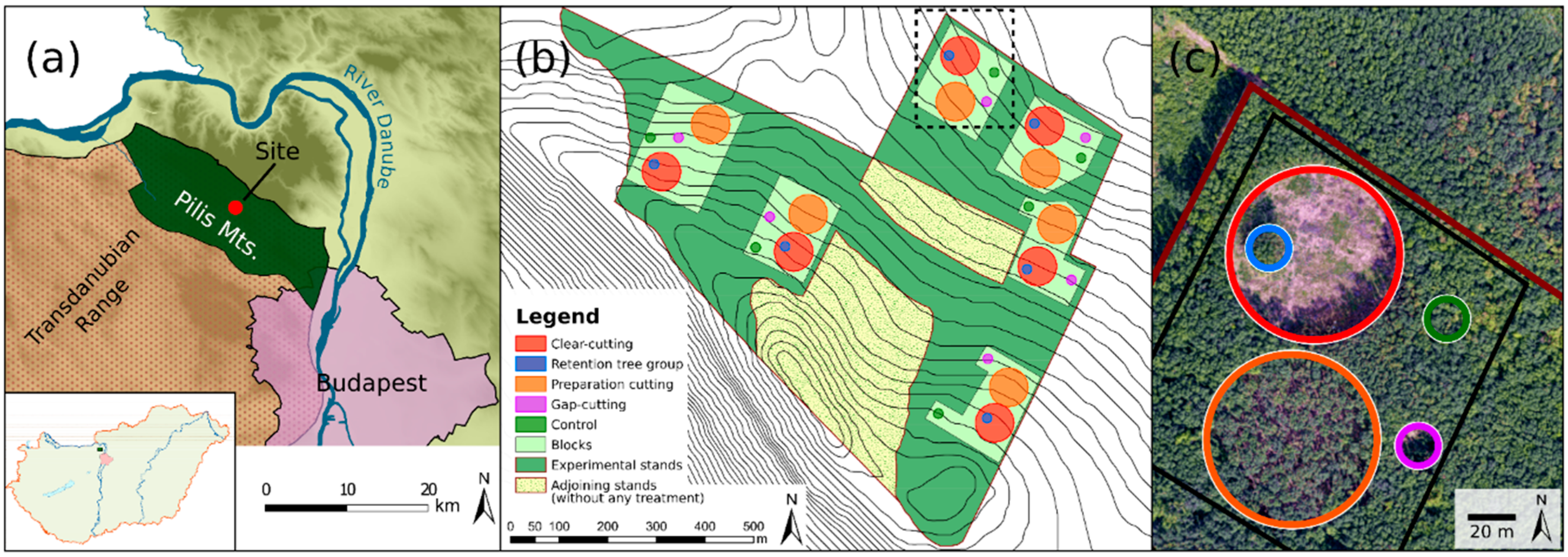
Figure 2.
Changes in means and interquartile ranges (IQR) of the relative values of the site condition variables among the forestry treatments in Pilis Mountains, Hungary, 2015. (a) Mean and (b) IQR of photosynthetically active radiation (PAR; μE m−2 s−1); (c) mean of relative diffuse light (DIFN; %); (d) mean and (e) IQR of air temperature (Tair; °C); (f) mean and (g) IQR of relative humidity (RH; %); (h) mean and (i) IQR of vapor pressure deficit (VPD; kPa); (j) mean and (k) IQR of soil temperature (Tsoil; °C); (l) mean of soil moisture (SWC; m3/m3); (m) total mass of collected litter on the surface (g/m2); (n) litter pH (pH in water); (o) gravimetric moisture content of litter samples (%); (p) soil pH (pH in water). The letter ‘d’ in the variable abbreviations refers to the differences from the mean values measured in the control plots. The treatment types are coded as follows: CC—clear-cutting; G—gap-cutting; P—preparation cutting; R—retention tree group. Full circles show the mean and vertical lines denote the standard deviation of the samples. Letters designate the significant differences among the treatments (all of the pairwise multiple comparisons based on the linear mixed effects models; Tukey-test, alpha = 0.05), while asterisks denote significant differences from the values measured at the control plots (linear mixed effects models without intercept, p < 0.05). The horizontal blue line shows the level of the control.

Figure 3.
Temporal variability of the selected microclimate variables among the experimental treatments and months in the Pilis Mountains, Hungary, 2015. (a) Mean of the photosynthetically active radiation ([PAR] μE m−2 s−1); (b) mean of vapor pressure deficit ([VPD] kPa); (c) mean of soil temperature ([Tsoil] °C); (d) mean of soil moisture ([SWC] m3/m3). The letter d in the variable abbreviations refers to the differences from the mean values measured in the control plots. Treatment types are coded as follows: CC—clear-cutting; G—gap-cutting; P—preparation cutting; R—retention tree group. Full circles show the mean and vertical lines denote the standard deviation of the samples. Letters designate the significant differences among the treatments and months (all of the pairwise multiple comparisons based on the linear mixed effects models: Tukey test, alpha = 0.05). The horizontal blue line shows the level of the control.
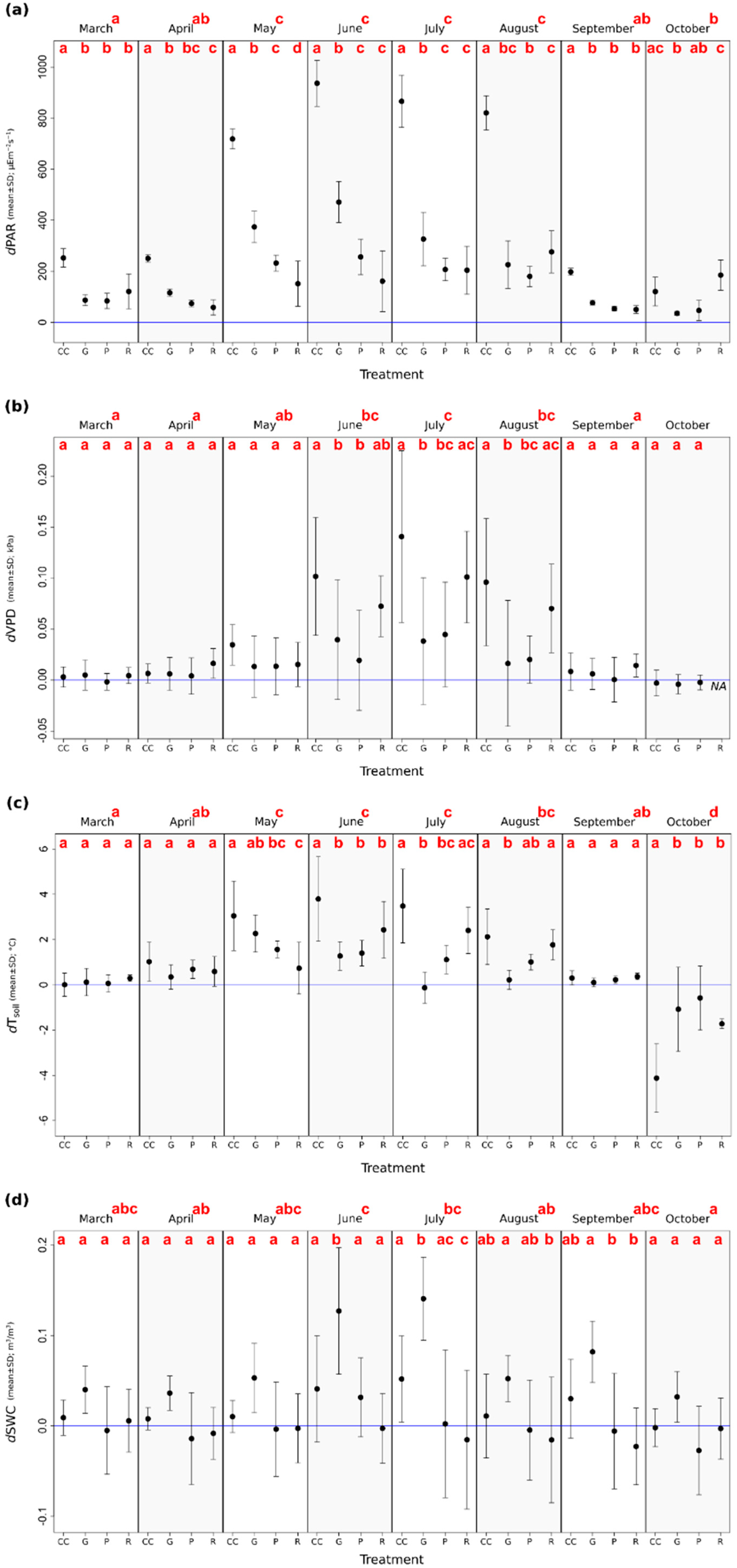
Figure 4.
Seasonal changes in selected soil and litter variables in Pilis Mountains, Hungary, 2015. (a) Total mass of collected litter on the surface (g/m2); (b) litter pH (pH in water); (c) gravimetric moisture content of litter samples (%); (d) soil pH (pH in water). The letter d in the variable abbreviations refers to the differences from the mean values measured in the ‘Control’ plots. Treatment types are coded as follows: CC—clear-cutting; G—gap-cutting; P—preparation cutting; R—retention tree group. Full circles show the mean and vertical lines denote the standard deviation of the samples. Letters designate the significant differences among the treatments (all of the pairwise multiple comparisons based on the linear mixed effects models; Tukey test, alpha = 0.05). The horizontal blue line shows the level of the control.

Figure 5.
Diurnal patterns of selected microclimate variables. Diurnal magnitudes of PAR (photosynthetically active radiation), VPD (vapor pressure deficit) and Tsoil (soil temperature) among treatments in the peak of the growing season (i.e., June, July, August; left) and during the transition period (March, April, September, October; right), respectively. Lines represent means calculated by LOWESS function (based on the 6 replicates for each variable per month), bands represent 95% confidence intervals. Colors are coding the treatments: control—green; clear-cutting—red; gap-cutting—purple; preparation cutting—orange and retention tree group—blue. Note that scales of y-axes vary between graphs.


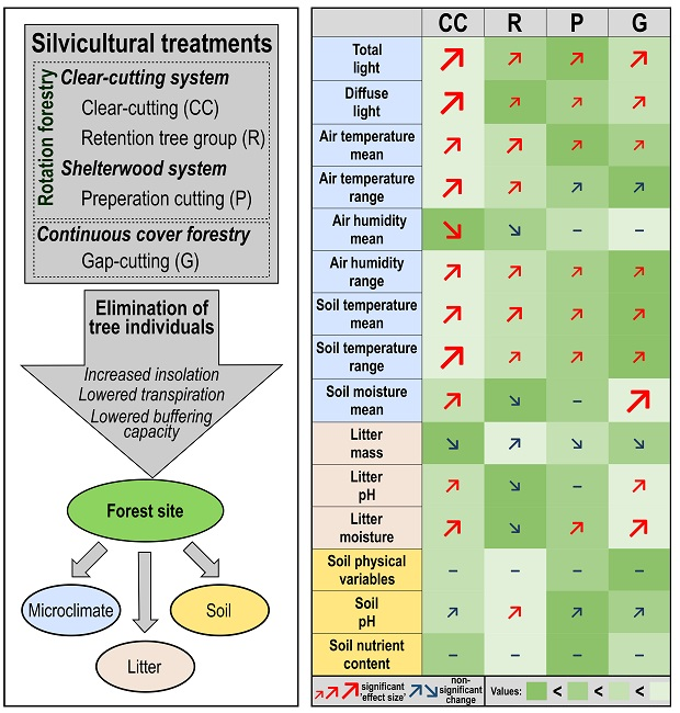
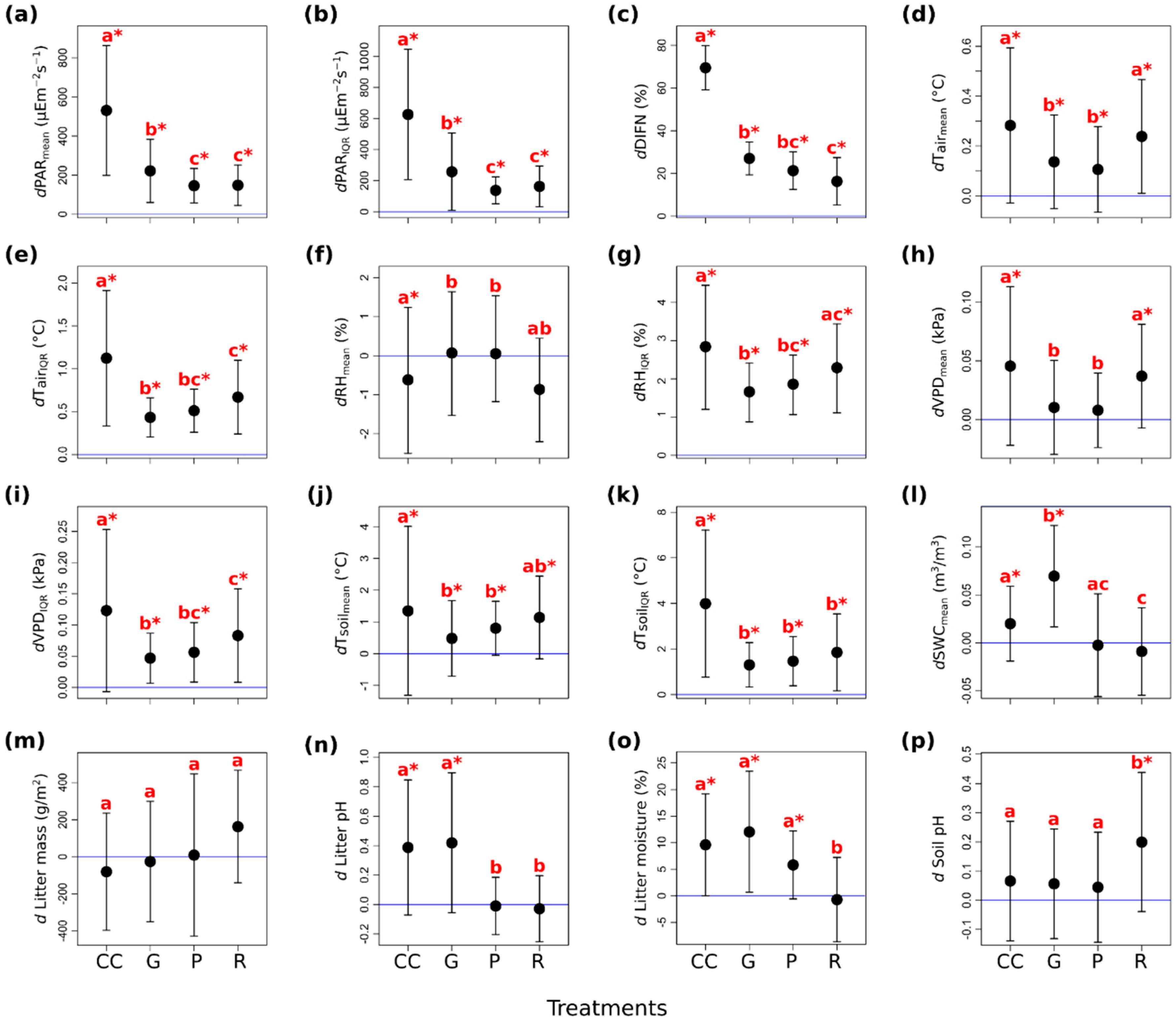
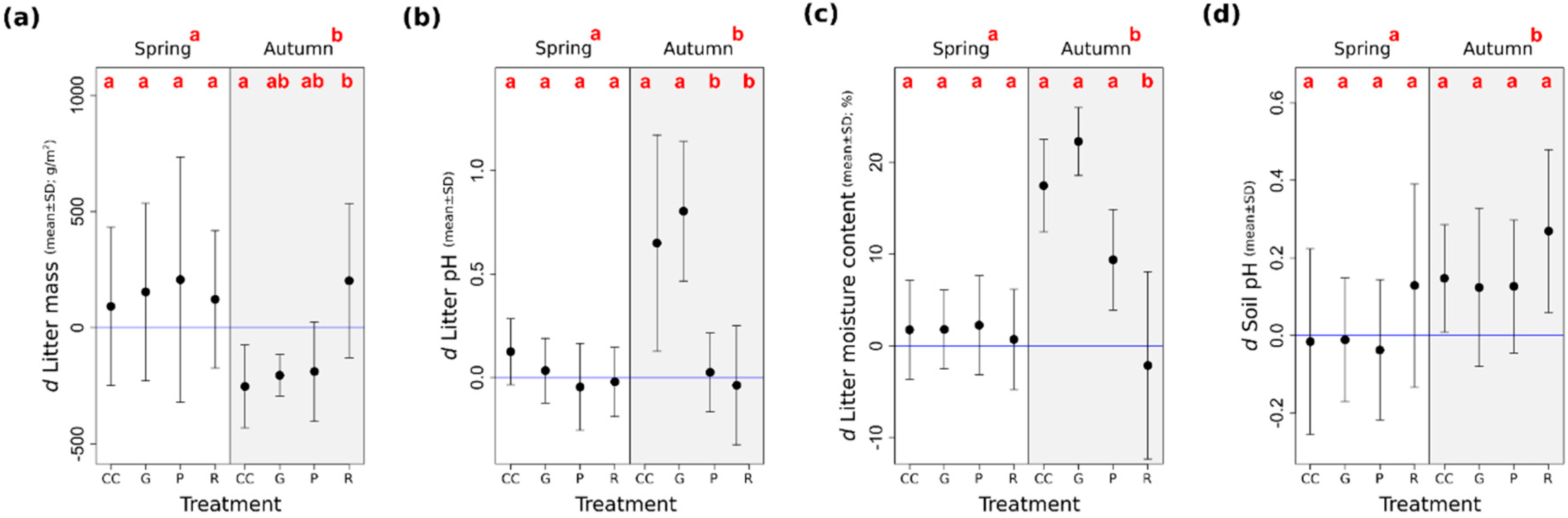
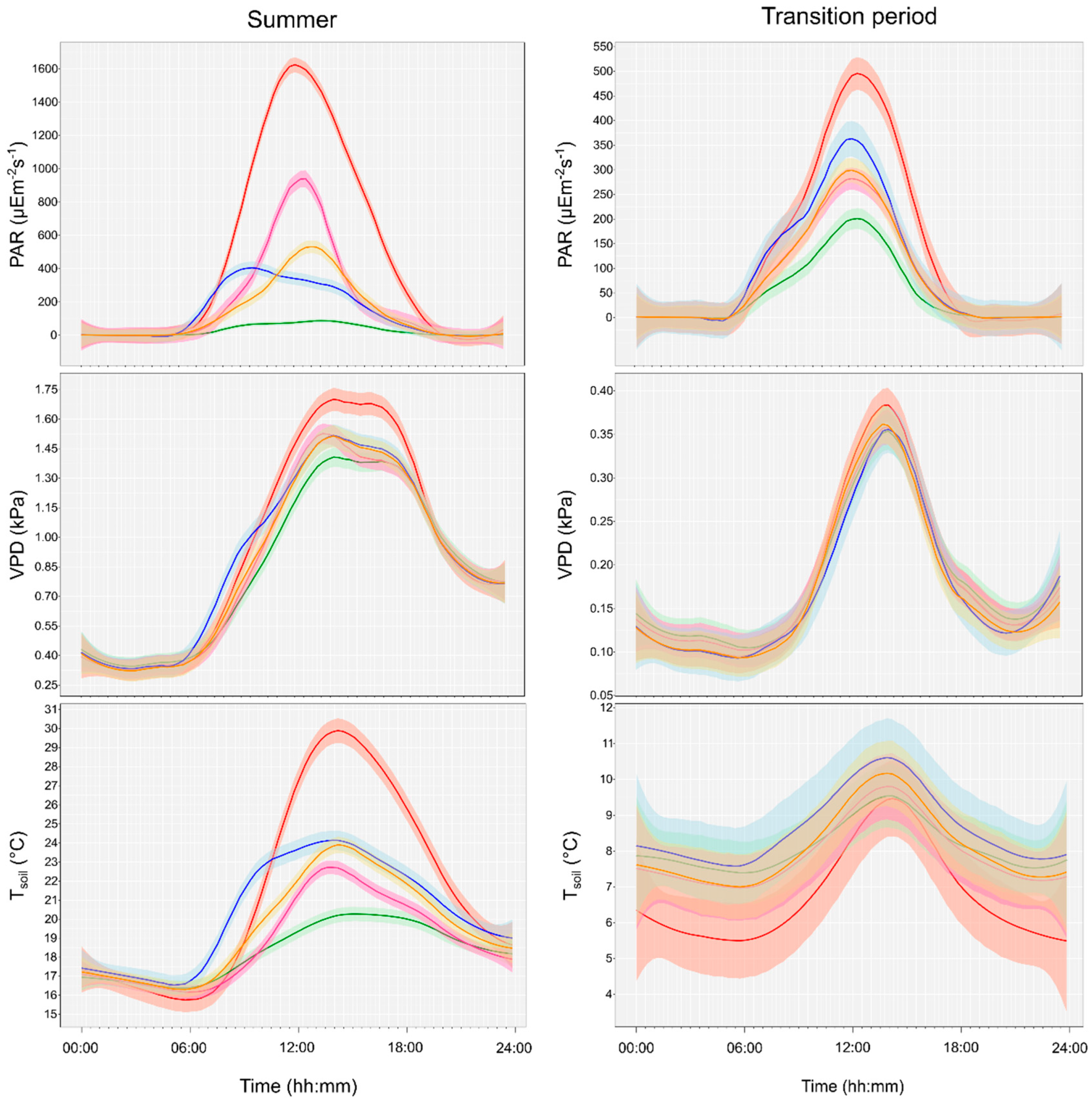
Table 1.
Characteristics of forest structure around the plots, before and after treatments. Structural attributes (mean ± standard deviation) presented here are the diameter at breast height ([DBH], cm), canopy height (m), basal area (m2 ha−1), and canopy closure (%). U—upper layer; S—sub-canopy layer; C—control; CC—clear-cutting; G—gap-cutting; P—preparation cutting; R—retention tree group. The mean and standard deviation were calculated based on the six replicates for each treatment type.
| Treatment | Pre-Treatment (2014) | Post-Treatment (2015) | ||||||||
|---|---|---|---|---|---|---|---|---|---|---|
| DBH | Height | Basal Area | Canopy Closure | Basal Area | Canopy Closure | |||||
| U | S | U | S | U | S | U | S | |||
| C | 28.0 ± 5.8 | 11.9 ± 3.8 | 20.9 ± 1.5 | 10.8 ± 3.5 | 29.32 ± 0.12 | 8.83 ± 0.10 | 89.8 ± 2.6 | 29.32 ± 0.12 | 8.83 ± 0.10 | 93.5 ± 3.9 |
| CC | 28.0 ± 5.7 | 11.8 ± 4.2 | 21.6 ± 1.6 | 10.4 ± 3.8 | 29.58 ± 6.47 | 9.98 ± 4.66 | 87.9 ± 3.6 | 0.00 | 0.00 | 2.5 ± 2.1 |
| G | 27.3 ± 5.3 | 12.5 ± 2.8 | 20.5 ± 1.1 | 11.2 ± 2.9 | 29.53 ± 9.03 | 9.33 ± 4.51 | 88.4 ± 4.4 | 0.00 | 0.00 | 44.8 ± 10.4 |
| P | 27.2 ± 5.3 | 10.9 ± 4.1 | 21.2 ± 1.4 | 10.0 ± 3.5 | 28.07 ± 2.10 | 8.03 ± 1.33 | 89.4 ± 4.4 | 19.67 ± 1.48 | 0.00 | 70.2 ± 6.9 |
| R | 27.3 ± 5.8 | 11.1 ± 3.4 | 20.4 ± 1.9 | 11.8 ± 3.9 | 30.47 ± 3.73 | 8.17 ± 2.35 | 88.7 ± 3.2 | 30.47 ± 3.73 | 8.17 ± 2.35 | 81.9 ± 9.2 |
Table 2.
The results of the linear mixed effects models performed for site condition variables. PAR—photosynthetically active radiation (μE m−2 s−1); DIFN—relative diffuse light (%); Tair—air temperature (°C); RH—relative humidity (%); VPD—vapor pressure deficit (kPa); Tsoil—soil temperature (°C); SWC—soil moisture (m3/m3); Litter mass—total mass of collected litter on the surface (g/m2); Litter pH—pH in water; Litter moisture content—gravimetric moisture content of litter samples (%); Soil pH—soil pH in water; hy—Kuron’s hygrscopicity (%); [SOC]—total soil carbon content (%); [N]—total nitrogen content (%); [PAL]—concentration of AL-soluble phosphorus (mg/100 g soil); [KAL]—concentration of AL-soluble potassium (mg/100 g soil). d refers to the difference from the values measured in the control plots. For modeling, 24 h means were used, except in the case of PAR, where the daytime (6:00–18:00 Coordinated Universal Time [UTC]) means were calculated.
| Dependent Variable | Model | Treatment | Time | Treatment: Time | |||||
|---|---|---|---|---|---|---|---|---|---|
| Chi2 | p | R2LR | F | p | F | p | F | p | |
| dPAR mean | 454.711 | <0.0001 | 0.922 | 225.579 | <0.0001 | 133.928 | <0.0001 | 8.941 | <0.0001 |
| dPAR IQR | 343.698 | <0.0001 | 0.852 | 114.259 | <0.0001 | 57.575 | <0.0001 | 6.292 | <0.0001 |
| dDIFN | 29.086 | <0.0001 | 0.766 | 21.699 | <0.0001 | - | - | - | - |
| dTair mean | 273.305 | <0.0001 | 0.781 | 21.888 | <0.0001 | 54.082 | <0.0001 | 4.903 | <0.0001 |
| dTair IQR | 265.160 | <0.0001 | 0.771 | 44.487 | <0.0001 | 47.139 | <0.0001 | 2.016 | 0.0086 |
| dRH mean | 46.096 | <0.0001 | 0.434 | 5.177 | 0.0021 | 2.939 | 0.0105 | 0.609 | 0.8866 |
| dRH IQR | 125.451 | <0.0001 | 0.569 | 14.054 | <0.0001 | 16.694 | <0.0001 | 1.275 | 0.2173 |
| dVPD mean | 122.668 | <0.0001 | 0.595 | 13.2782 | <0.0001 | 13.9286 | <0.0001 | 1.8528 | 0.0267 |
| dVPD IQR | 259.555 | <0.0001 | 0.823 | 37.279 | <0.0001 | 63.435 | <0.0001 | 5.491 | <0.0001 |
| dTsoil mean | 261.975 | <0.0001 | 0.768 | 9.107 | <0.0001 | 44.611 | <0.0001 | 7.368 | <0.0001 |
| dTsoil IQR | 201.537 | <0.0001 | 0.674 | 24.397 | <0.0001 | 24.166 | <0.0001 | 3.248 | <0.0001 |
| dSWC mean | 109.965 | <0.0001 | 0.534 | 29.145 | <0.0001 | 2.3129 | 0.0292 | 1.089 | 0.3666 |
| dLitter mass | 21.338 | 0.0033 | 0.424 | 2.164 | 0.1097 | 10.812 | 0.0057 | 1.955 | 0.1387 |
| dLitter pH | 35.390 | <0.0001 | 0.524 | 8.888 | 0.0002 | 8.685 | 0.0057 | 3.646 | 0.0218 |
| dLitter moisture | 47.003 | <0.0001 | 0.624 | 9.318 | 0.0001 | 16.478 | 0.0003 | 7.355 | 0.0009 |
| dSoil pH | 23.863 | 0.0012 | 0.544 | 3.633 | 0.0221 | 15.754 | 0.0003 | 0.041 | 0.9889 |
| dhy | 10.428 | 0.1656 | 0.219 | 2.824 | 0.0528 | 0.115 | 0.7369 | 0.426 | 0.7358 |
| d[SOC] | 5.008 | 0.6590 | 0.352 | 1.202 | 0.3242 | 0.159 | 0.6930 | 0.223 | 0.8799 |
| d[N] | 3.415 | 0.8442 | 0.357 | 0.912 | 0.4451 | 0.008 | 0.9316 | 0.074 | 0.9738 |
| d[PAL] | 10.308 | 0.1718 | 0.388 | 1.936 | 0.1418 | 1.034 | 0.3163 | 0.965 | 0.4200 |
| d[KAL] | 12.735 | 0.0788 | 0.299 | 1.641 | 0.1821 | 6.956 | 0.0124 | 0.173 | 0.9143 |
© 2018 by the authors. Licensee MDPI, Basel, Switzerland. This article is an open access article distributed under the terms and conditions of the Creative Commons Attribution (CC BY) license (http://creativecommons.org/licenses/by/4.0/).
Share and Cite
MDPI and ACS Style
Kovács, B.; Tinya, F.; Guba, E.; Németh, C.; Sass, V.; Bidló, A.; Ódor, P. The Short-Term Effects of Experimental Forestry Treatments on Site Conditions in an Oak–Hornbeam Forest. Forests 2018, 9, 406. https://doi.org/10.3390/f9070406
AMA Style
Kovács B, Tinya F, Guba E, Németh C, Sass V, Bidló A, Ódor P. The Short-Term Effects of Experimental Forestry Treatments on Site Conditions in an Oak–Hornbeam Forest. Forests. 2018; 9(7):406. https://doi.org/10.3390/f9070406
Chicago/Turabian StyleKovács, Bence, Flóra Tinya, Erika Guba, Csaba Németh, Vivien Sass, András Bidló, and Péter Ódor. 2018. "The Short-Term Effects of Experimental Forestry Treatments on Site Conditions in an Oak–Hornbeam Forest" Forests 9, no. 7: 406. https://doi.org/10.3390/f9070406
Note that from the first issue of 2016, this journal uses article numbers instead of page numbers. See further details here.