Modeling Production Processes in Forest Stands: An Adaptation of the Solow Growth Model

1
Sukachev Institute of Forest SB RAS, Federal Research Center “Krasnoyarsk Science Center SB RAS”, Akademgorodok 50-28, 660036 Krasnoyarsk, Russia
2
Institute of Biophysics SB RAS, Federal Research Center “Krasnoyarsk Science Center SB RAS”, Akademgorodok 50-50, 660036 Krasnoyarsk, Russia
*
Author to whom correspondence should be addressed.
Forests 2018, 9(7), 391; https://doi.org/10.3390/f9070391
Submission received: 28 May 2018
/
Revised: 27 June 2018
/
Accepted: 28 June 2018
/
Published: 2 July 2018
(This article belongs to the Special Issue Simulation Modeling of Forest Ecosystems)
Abstract
:The model of forest stand growth proposed in this study is based on R. Solow’s model of economic growth. The variables introduced into the model are the “capital” (the phytomass of the non-synthesizing tree components in the stand—the stem, roots, and branches) and the “labor” (the phytomass of the photosynthesizing tree components in the stand—leaves or needles). Root phytomass is calculated with a special independent model. The process of energy production by the trees is described with the Cobb-Douglas equation. The proposed approach is used to describe growth processes in the forest stands comprising various species in Siberia and the age dynamics of net primary production. The model can explain a number of effects (such as death of the forest stand after the needles have been consumed by defoliating insects) that cannot be explained by standard logistic models.
1. Introduction
The growth of individuals and populations can be presented as the totality of all births (the birth of a new individual or a change in the population density, biomass of an individual, or biomass of the entire population) and dissipation (the death of an individual or a population). Growth processes are usually described by using logistic models, including the Verhulst, Gompertz, Mitscherlich, Chapman-Richards functions, etc. [1,2,3,4,5,6,7,8]. Such models describe the growth process with one independent variable x, which characterizes the state of the system (the number of individuals in the population, the mass of one individual or the entire population) and a set of free parameters such as birth rates or biomass synthesis rates.
However, descriptions of processes observed in forest stands by growth models are not in complete agreement with the real processes occurring in the forest.
For instance, the death of the forest stand is as natural as its growth, and mortality processes should be described in the model too [9]. According to logistic models, consumption at an arbitrary time of any amount of phytomass that is smaller than its current value never causes the death of a forest stand. However, a fir tree (Abies sibirica Ledeb.) dies if larvae of the Siberian silk moth (Dendrolimus sibiricus Tschetv.) have consumed all its needles, although the phytomass of the needles constitutes about 3% of the total phytomass of a 100-year-old tree [10,11].
In a valid model of forest stand growth, there must be a steady state with x = 0, which describes a rather common situation when the forest is dead or cut down, but no reforestation occurs. In the logistic models, however, there is only one steady state, with x = A, while the state with x = 0 is not steady.
Logistic models only evaluate phytomass growth rate, but GPP (gross primary production) and NPP (net primary production) cannot be determined by using those models. Phytomass loss in the forest stand, a very significant ecological parameter, cannot be estimated either. Finally, those growth models do not take into account the effects of climate factors on forest stand growth.
Today, the most common approach to estimating the NPP of forest stands is the use of balance equations, which contain the data on the increment, fall-off, and loss of forest stand phytomass, standing timber volume, and allometries. However, despite the apparent conceptual simplicity of balance equations, it is very difficult to exactly evaluate the NPP by using the forest inventory data. Exact evaluations are only possible regarding the increment in the standing timber volume or phytomass between ages T and T + ΔT. The increments in branch and leaf phytomass can be evaluated with lower accuracy [12,13]. The main challenge associated with NPP evaluation is the difficulty or even impossibility of measuring the phytomass and phytomass increment of the tree roots. Another challenge is the evaluation of the phytomass loss, as there are no exact data on the rates of dying of roots, branches, and bark [14,15,16].
In many cases, the data on the phytomass of tree parts and changes in the phytomass are lacking, and the only available data are inventories of the standing timber or measurements of the height and diameter of the trees in the stand. Then, calculations of the phytomass of each tree part and subsequent NPP evaluations are performed using regression equations that characterize relationships between the phytomasses of tree parts and the standing timber stock or tree diameters and heights [10,11,17,18,19,20]. For instance, evaluations of the NPP of Russian forests based on these approaches vary widely [21].
In the present study, growth processes of tree stands are estimated using a model based on R. Solow’s model of economic growth, which is more complex than logistic models and which includes two independent variables describing processes of product generation and accumulation in the model system. The Solow growth model [22] assumes that manufacturability of products is related to the presence of two major factors: capital, K (total costs of equipment, manufacturing premises, transport, current assets, etc.) and labor force, L. The Solow model also includes the production function, which characterizes production volume, Y, as related to values of K and L [22,23]. According to Solow’s model, a certain percentage of the revenue received from the sale of the products is consumed, and the other fraction is invested into the manufacturing system, increasing the amount of the capital and compensating for its loss due to depreciation of the equipment and manufacturing premises. The production volume in the next manufacturing cycle is determined by the new values of K and L.
2. Materials and Methods
2.1. The EcoSolow Model of Production Processes in the Forest Stand
In this study, we have adapted Solow’s model of economic growth to describe the growth of forest stands and estimate their NPP. In our adaptation of the Solow model—the EcoSolow model (ESM), the process of phytomass growth in a forest stand is regarded as analogous to a manufacturing process, which is determined by two production factors: capital and labor. In the ESM, capital, K, consists of the non-photosynthesizing components of the phytomass—tree stem, roots, and branches, and labor force, L, is represented by leaves (or needles), which carry out photosynthesis. The GPP energy produced during photosynthesis is partly expended for the current “consumption” (respiration) of the plant, and the other part is “invested” and transformed into new phytomass, which is distributed between the non-photosynthesizing components of the trees and their photosynthetic apparatus. Tree mortality in the ESM is regarded as analogous to capital depreciation (wear and tear of the equipment etc.) in the manufacturing process.
The non-photosynthesizing component, K(T), of the forest stand of age T comprises phytomasses of stems MS(T), roots MR(T), and branches MB(T):
The photosynthesizing component consists of needles (leaves) of the trees in the forest stand with phytomass ML(T). Energy production, GPP, by trees during photosynthesis will be described by the Cobb-Douglas production function [24,25]:
where T is the forest stand age, A, and α and β are coefficients.
Let us then consider the simplest case, when in Equation (2), , and, hence, in Equation (2) there are only two free parameters: A and α.
Part of the energy generated during photosynthesis is expended for maintaining the current functions of the trees (in fact, respiration). These expenditures, Z(T), will be assumed to be related to the total phytomass of the stand, :
where is the function of current expenditures.
In the simplest case, current expenditures can be assumed to be directly proportional to the stand phytomass, i.e., . Coefficient s can be regarded as expenditure for the functioning of the unit phytomass (we assume that these expenditures do not differ between tree components).
The difference between production Y and current expenditures of energy Z(T) will characterize net primary production, NPP:
In Equation (4), the values of coefficients of elasticity α and (1 − α) characterize an increase in the photosynthesis rate of the trees with an increase in the per unit values of K and ML:
As can be inferred from Equation (2), production cannot occur if at least one production factor, K or L, is equal to zero. Ecologically speaking, the death of the foliage due to some reasons (insect damage, fire, effects of pollutants, etc.) stops the “production” and leads to the death of the tree irrespective of the value of K of the non-photosynthesizing phytomass. The condition that follows from Equation (2) is ecologically valid, in contrast to the ecologically incorrect solution for the logistic models. This condition enables describing the processes of tree death caused by critical natural or human-induced events.
If net primary production of the stand at age T is completely “invested” in the stand phytomass increment, values of K(T) and ML(T), and coefficients A, α, s of Equation (4) must be known to be able to model the production process in the forest stand.
To verify the EcoSolow model, let us consider the following balance equation for the phytomass of the forest stand of adjacent ages T and T + ΔT. For coniferous species, the youngest age classes are ΔT = 20 years, and for hardwood species, ΔT = 10 years:
where NPP (T, T + ΔT) is primary production of the forest stand aged between T and T + ΔT years; M(T) and M (T + ΔT) are phytomasses of the forest stand aged T and T + ΔT; D(ΔT) and W(ΔT) are phytomass loss and fall-off for ΔT years.
Let us rewrite Equation (5) as follows:
By inserting the NPP value from Equation (4) into the left-hand part of Equation (6), we obtain a recurrent equation relating the phytomasses of the forest stand of adjacent ages T and T + ΔT:
To accurately evaluate the forest stand phytomass, one needs to know all phytomass values in Equation (7), including root phytomass, and determine the distribution of the phytomass synthesized at ages between T and T + ΔT between the photosynthesizing and non-photosynthesizing components (Equation (7) does not enable this evaluation). Unfortunately, forest inventories usually either contain no data on root phytomass, as it is very difficult to measure it in the field, or present results of calculations performed by unreliable methods [26,27,28,29,30]. In this study, calculations of root phytomass were based on the data on the phytomass of aboveground components and the phytomass distribution between the photosynthesizing and non-photosynthesizing components. We calculated the root phytomass by using a model proposed previously, in which root phytomass of a tree or a forest stand was estimated from the data on the phytomasses of the stem (with the bark), branches and leaves (needles) [31,32,33]. The Appendix A section contains the description of the model used to calculate the root phytomass in the forest stand and the distribution of the phytomass at age T + ΔT between the photosynthesizing and non-photosynthesizing components.
The leaf (needle) fall-off is determined by using Equation . ML(T) is needle phytomass, Θ is the average lifespan of the foliage. For the birch, aspen, and larch, Θ = 1 year. For conifers, Θ varies between 2 and 6 years. Then the ML(T)/θ ratio is the needle phytomass loss over 1 year, and is the mass of the leaf (needle) fall-off over the time ΔT, between two successive inventories.
The loss of trees in the forest stand, in the case when the stand density ρ(T) and total phytomass are known for each age, is estimated as follows:
If the time series of the phytomass components in the forest stand, MS(T), MR(T), MB(T), and ML(T), and the time series of the fall-off D(ΔT) and the loss W(ΔT) of the forest stand phytomass are available, Equation (7) can be regarded as a nonlinear regression equation with unknown coefficients A, α and s. Coefficients A, α and s in Equation (7) were calculated using the least squares method, with a nonlinear regression model. The coefficient of determination R2 is used to evaluate the quality of data approximation by model Equation (7).
2.2. Model Data
Inventory data on single-species even-aged pine, larch, spruce, fir, and birch stands in Siberia reported by different authors were collected in summaries [10,11]. The data on the stand density, ρ, and phytomass of aboveground components are given for each stand at different ages. Table 1 lists typical inventory data on phytomasses of pine stands of different ages in taiga forests.
3. Results
In the adaptation of the Solow model—the EcoSolow model (ESM)—proposed in this study, the process of phytomass growth in a forest stand is regarded as analogous to a manufacturing process. Capital, K, consists of the non-photosynthesizing components of the phytomass—tree stem, roots, and branches, and labor force, L, is represented by leaves (or needles), which carry out photosynthesis. Figure 1 shows estimations of growth dynamics of pine stands in Siberia calculated with the EcoSolow model. Inventory data and model calculations are evidently in good agreement (coefficients of determination R2 are higher than 0.98).
The ESM can be used to describe the nonmonotonic phytomass change observed in forest ecosystems, when, having reached its peak value at a certain age, the phytomass begins decreasing.
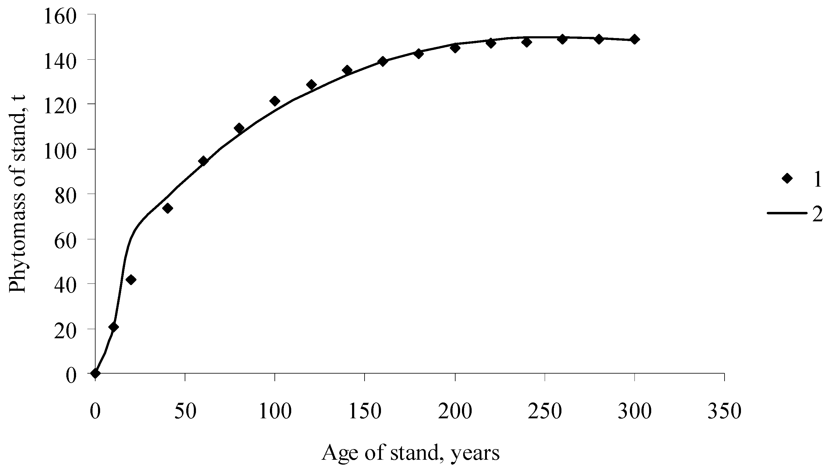
How do the calculations with the EcoSolow model differ from the NPP calculations with the balanced model (5)? Figure 2 and Figure 3 show the curves of the temporal growth dynamics of forest stand phytomass (including the root phytomass) and the NPP calculated with the balance model and the EcoSolow model. Calculations of the NPP by different methods yielded very similar results (particularly for older ages). However, in contrast to the nonparametric balance method of NPP calculation, the EcoSolow model provides estimations of three free parameters, A, α, and s. By analyzing the relationships between these parameters and the tree species and environmental conditions, one can obtain more information on the photosynthetic processes in woody plants.
We certainly do not know the “true” NPP curve, which could be compared to the ESM. The data in Figure 3 show that calculations based on the ESM and on the balanced model yield similar results. We did not attempt to force the ESM to fit the balanced model. Figure 3 shows that the NPP curves are similar. However, the main difference between the balanced model and the ESM is that the balanced model is a nonparametric one and it cannot be used to estimate changes in the NPP depending on the species and habitat. The ESM is a parametric model with parameters A, α, s and can be used to compare different tree stands using these parameters and correlate the parameters with the tree species and characteristics of the habitats. That is why the ESM is more suitable for analyzing growth processes of trees.
The approach proposed in this study description of growth processes in forest stands as analogous to manufacturing of products can be considered as an alternative to growth model calculations. The EcoSolow model is able to describe different events occurring in the forest (such as death of trees in forest stands), which cannot be explained by logistic models.
4. Discussion
Table 2 gives the values of the ESM parameters for different stands in the Siberian taiga forests, where the maximal values of coefficient A are characteristic of such deciduous species as larch and birch. For the Scots pine and the Siberian fir, parameters of the EcoSolow model are similar for forest stands growing under different climatic conditions.
As can be seen from the data in Table 2, for all tree species the elasticity (1 − α) in changing the photosynthesizing phytomass is significantly higher than the non-photosynthesizing phytomass elasticity. Thus, the NPP of the trees is less influenced by changes in the value of K than by changes in the mass of the photosynthesizing apparatus, ML.
If, initially, we assumed that , results of calculations showed that in this version of the model, α + β = 1.05, and this is very close to 1 (Table 2). Thus, we do not need to introduce the additional free parameter, β, into the model.
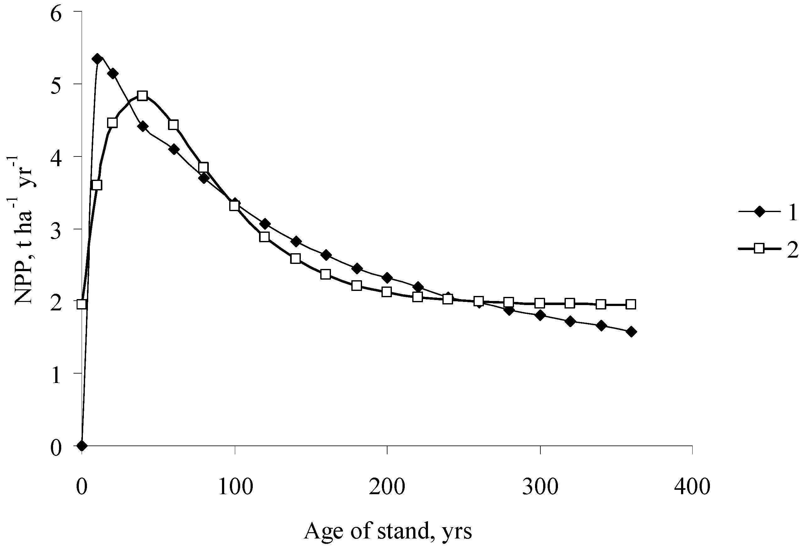
Figure 4 shows the age dynamics of the NPP of forest stands calculated from the values obtained for coefficients A, α, and s. The graph shows that the age trends of the NPP of pine stands (with the NPP maximum at the age of 40 years and NPP minimum at older ages up to 300 years) are similar for the stands growing in different geographical zones.
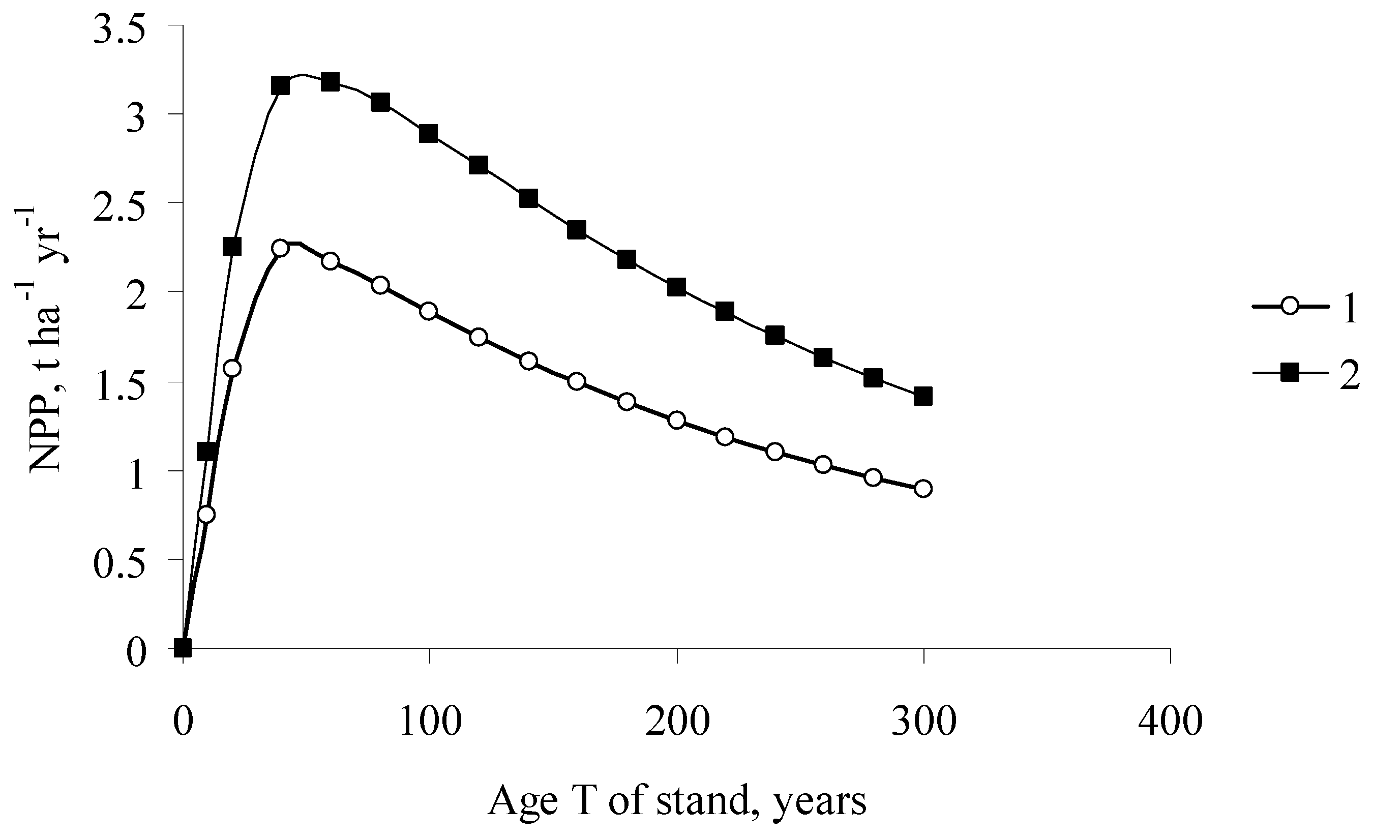
However, the absolute NPP values of the pine stands of all ages are higher for the stands growing in more favorable climatic conditions. The age dynamics of NPP were also similar for the single-species even-aged stands of various tree species in Siberia (Figure 5).
Note that for the dominant Siberian taiga species fir and larch, the NPP values are quite close in the same age group, although the characteristic lifespans of their needles differ considerably.
Since we know the values of GPP and NPP, we can characterize the effectiveness of the photosynthetic process as . It is obvious that , and that the closer the value of ŋ(T) to unity, the more effectively photosynthesis produces energy. Figure 6 shows the dynamics of parameters of photosynthesis effectiveness for pine stands in different geographical regions of Siberia. The effectiveness of photosynthesis monotonically decreases with the stand age. Interestingly, the highest effectiveness of photosynthesis was shown by the stands in the north taiga zone and the lowest by the stands in South Siberia.
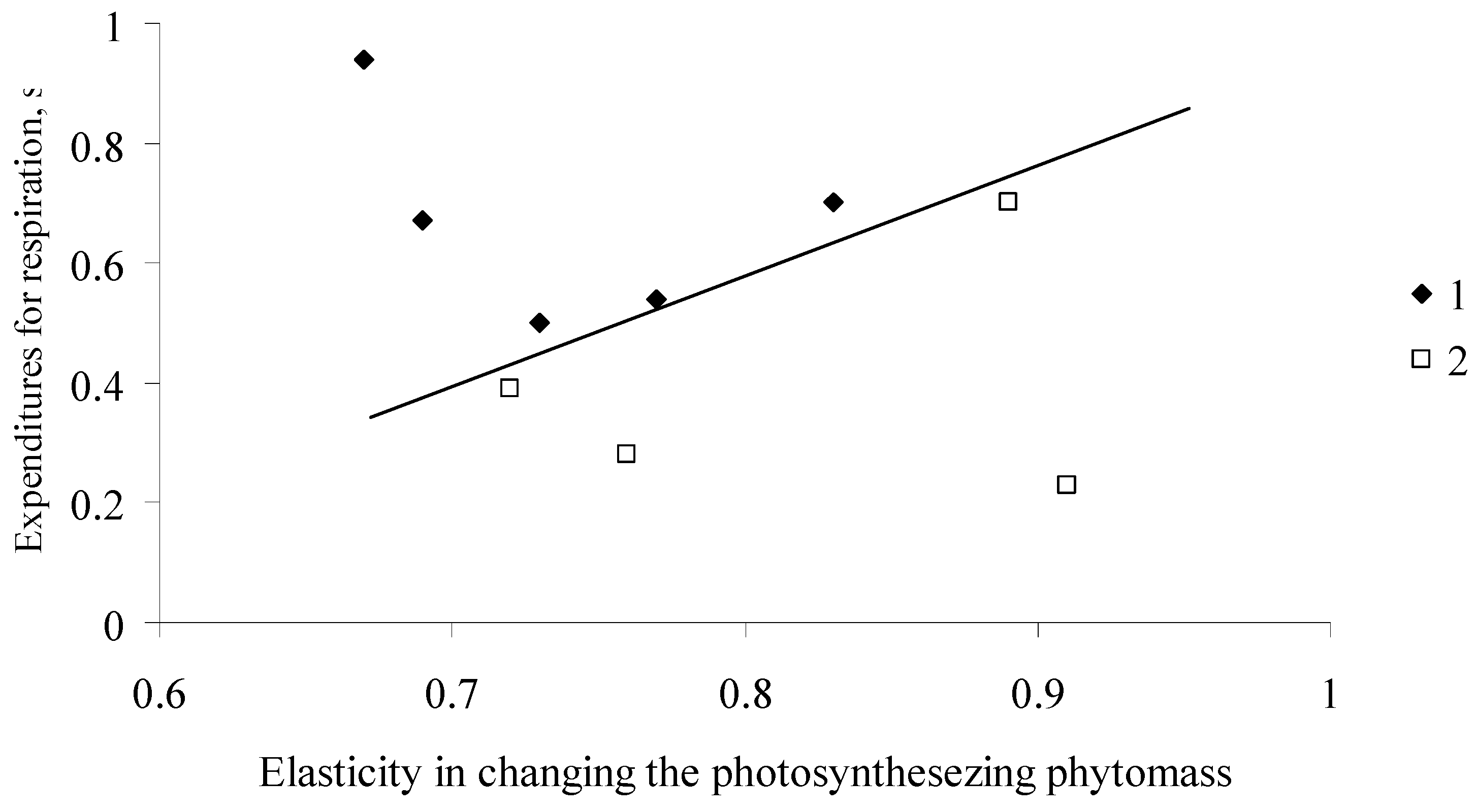
Figure 7, in the plane, shows the values of parameters of forest stands consisting of different tree species in Siberia. Here, we can differentiate between the regions of values α and s for the south and north of Siberia. North and South Siberia differ quite substantially in their average winter and summer temperatures and total solar irradiance values.
For the trees in the north of Siberia, the values of (1 − α), which characterize changes in the photosynthesis rate with the increase in the photosynthesizing phytomass, are greater, while the values of coefficient s, which characterizes expenditures for respiration, are smaller.
Thus, in the northern regions of Siberia, a rather small increase in needle phytomass will cause a considerable increase in the photosynthesis rate, and this may be a factor of a fast increase in the forest stand phytomass during the years with favorable weather conditions. Trees growing in the less severe climate of South Siberia have somewhat lower values of coefficients (1 − α), and the response of the photosynthesizing system to the increase in the mass of the photosynthesizing apparatus is weaker.
5. Conclusions
Can growth processes in ecosystems be regarded as replicas of economic processes? No, definitely not. While economic models prove the existence of a steady trajectory of stationary growth, the ecological model proposed in this study describes the finite limited growth of phytomass. Despite the differences between economic and ecological production models, economic principles applied to ecological production models seem to be more appropriate for the description of the processes occurring in forest ecosystems than the basic principles of “classical” growth models. Moreover, the ESM can be modified quite easily to enable detailed modeling of growth processes in forest stands as related to the species of the woody plants and landscape and climatic conditions in their habitats.
The Solow model is a non-closed model (that is, not all variables are determined within the model), and its free variable is labor force, L, which is determined independently by the Malthusian Equation [22]. In the ESM, the mass of the photosynthetic component, ML, is closed, and it is related to the amount of the “phyto-capital” and coefficient b of the Zipf-Pareto equation, which describes the competitive distribution of the phytomass of the forest stand among its structural components. However, the ESM is non-closed regarding the tree loss function, which is given by the independent Equation (8). This is a considerable limitation of the EcoSolow model, and, maybe, we should introduce an additional limitation on the amount of phytomass at age T, which may enable tree loss processes in the forest stand within the framework of the model. The EcoSolow model may also be improved by introducing a delay in the energy production process during photosynthesis relative to the phytomass accumulation process. Economic models of production include a corresponding delay [34].
The climate factor in the ESM can be regarded as analogous to the factor of technological advances in economic models, characterized in the Solow model by the value of coefficient A in (2). However, economic models do not contain any factor analogous to the effects of weather conditions, which change from year to year, on forest stand growth, causing high-frequency variations (characteristically occurring every several years) in the radial growth of tree stems and height increments. The effects of climate conditions in the ESM can be taken into account by specifying exogenously the functions of climate influences on model coefficient A. However, this is associated with a certain arbitrariness in the description of the growth processes.
A very interesting problem to solve is construction of an EcoSolow model suitable for describing growth processes in mixed forests. An additive EcoSolow model that describes growth processes separately for every species constituting the stand is unable to take into account diverse interactions (competition, cooperation, commensalism, amensalism) between trees of different species. Therefore, EcoSolow models that will take into account interactions between species in mixed forest stands should be constructed.
EcoSolow models taking into account landscape and soil properties of the region could be of interest. Comparison of the growth models for the north and south taiga suggests that landscape and soil properties could be reflected in the values of coefficients in Equation (7). The effects of forest management (such as improvement cutting) could be regarded as phytomass loss at a certain stage of forest development. Whether the values of the model coefficients would remain the same is a question to be answered in future studies.
Thus, despite the differences between the economic and ecological production models, the principles of the proposed “manufacturing” ecological model seem to be more appropriate for describing processes occurring in forest ecosystems than the basic principles of balanced growth models. Moreover, the ESM can be modified quite easily to enable detailed modeling of growth processes in forest stands as dependent on the tree species, landscape and climate conditions in the habitats of the trees.
Author Contributions
V. Soukhovolsky is responsible for the idea to use the Solow model for description of growth processes in forest stands as analogous to manufacturing of products; Y. Ivanova analyzed the data and wrote the main part of the paper.
Funding
The research was funded by RFBR grant number No. 18-04-00119.
Conflicts of Interest
The authors declare no conflict of interest.
Appendix A
Calculating the root phytomass in a forest stand based on the data on the phytomasses of the stem with the bark, branches, and leaves (needles).
The total phytomass of the non-photosynthesizing components of the forest stand, K(T), includes root phytomass (usually 15–29% of the total phytomass in the stand). However, the root phytomass of the trees in the stand usually cannot be measured in field studies. It was previously proposed to describe the distribution of the phytomass among tree or forest stand components by the Zipf-Pareto equation in the rank form [31,32,33]:
Or
where i is the rank of the phytomass component (the stem with the bark, roots, branches, leaves or needles) (starting with the component that has the greatest phytomass, M1); Mi is the phytomass of the rank i component; and b(T) is the coefficient characterizing percentages of phytomasses of different ranks.
If b(T) → 0, the phytomasses of all components are approximately equal to each other; when b(T) is increased, the phytomass of the rank 1 component (usually tree stems) is considerably greater than the phytomass of any other tree component in the stand. Regarding (A2) as a regression equation with the known values of the phytomass and ranks of phytomasses of aboveground components (stems, branches, leaves (needles)), one can find coefficient b and then calculate root phytomass:
From (1S) one can derive a formula for the total phytomass of the stand, M(T), at any age:
Function G(b(T)) is not related to the current values of the stand phytomass; it characterizes the proportions of phytomass components at age T. As the rank of the phytomass of leaves (needles) of forest stands aged above 10 years is always equal to 4 [33], by taking into account (A1) and (A4) we obtain:
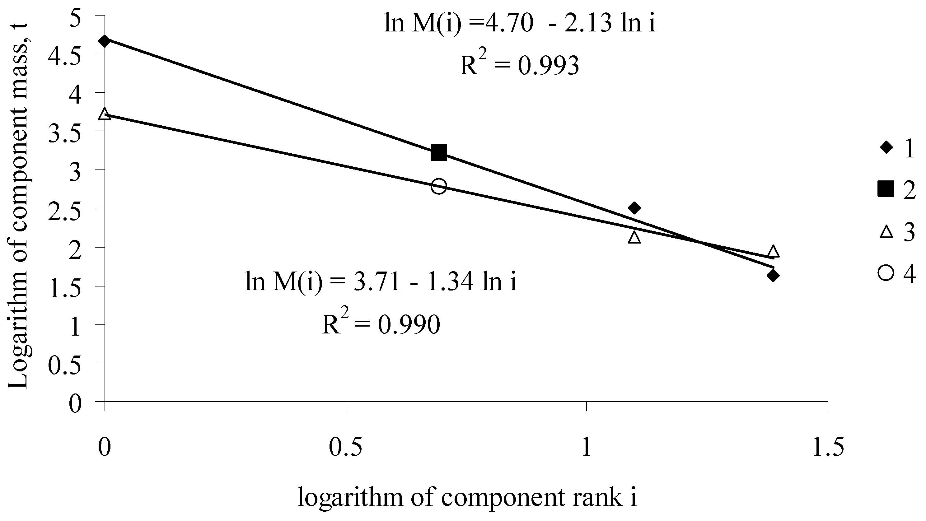
Thus, knowing function b(T), from the Zipf-Pareto equation for phytomass distribution, we can obtain the values of “phyto-capital” K(T) and the mass of the photosynthetic apparatus ML(T) for the forest stand of age T. Figure A1 shows a typical function of the rank distribution of fir stand phytomass components at ages between 40 and 300 years.
Figure A1.
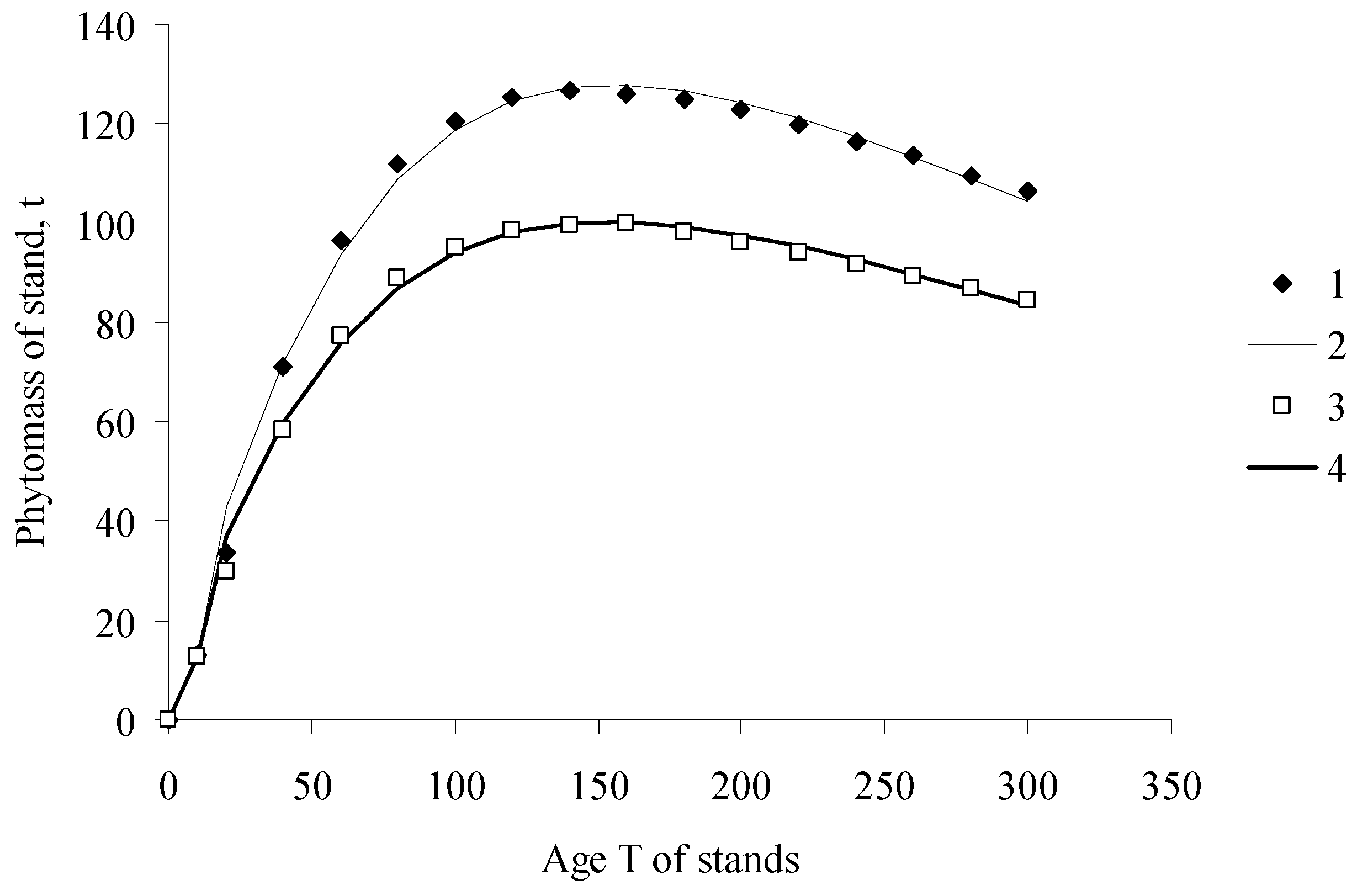
Functions of phytomass distribution among components of the Siberian fir Abies sibirica Ldb. stand (the West Sayan Mountains, the upper reaches of the Kebezh River, 52°N, 89°E) at ages of 40 and 300 years. (1) aboveground components of tree phytomass in the 300-year-old stand; (2) calculated root phytomass in the 300-year-old stand; (3) aboveground components of tree phytomass in the 40-year-old stand; (4) calculated root phytomass in the 40-year-old stand [10].
Figure A1.
Functions of phytomass distribution among components of the Siberian fir Abies sibirica Ldb. stand (the West Sayan Mountains, the upper reaches of the Kebezh River, 52°N, 89°E) at ages of 40 and 300 years. (1) aboveground components of tree phytomass in the 300-year-old stand; (2) calculated root phytomass in the 300-year-old stand; (3) aboveground components of tree phytomass in the 40-year-old stand; (4) calculated root phytomass in the 40-year-old stand [10].

Equation (A2) can be regarded as a regression equation with the known values of phytomasses and ranks of phytomasses, for which one should calculate its coefficients. Assuming that the root phytomass of the Siberian fir is a rank 2 component, the values of the phytomasses of aboveground tree components are described with high accuracy (R2 > 0.99) by Equation (A2) (Figure A1). Knowing coefficients of regression Equation (A2), one can calculate root phytomass.
The method described above was used to determine the ranks of roots and to calculate the values of root phytomass in forest stands. Is Equation (A2) sufficiently accurate? Figure A2 shows the distribution of coefficients of determination, R2, for the data on the distribution of phytomass in forest stands among tree components.
Figure A2.
The distribution of the coefficient of determination R2 of the linearized Zipf-Pareto Equation (A2) for the phytomass distribution among tree components.
Figure A2.
The distribution of the coefficient of determination R2 of the linearized Zipf-Pareto Equation (A2) for the phytomass distribution among tree components.
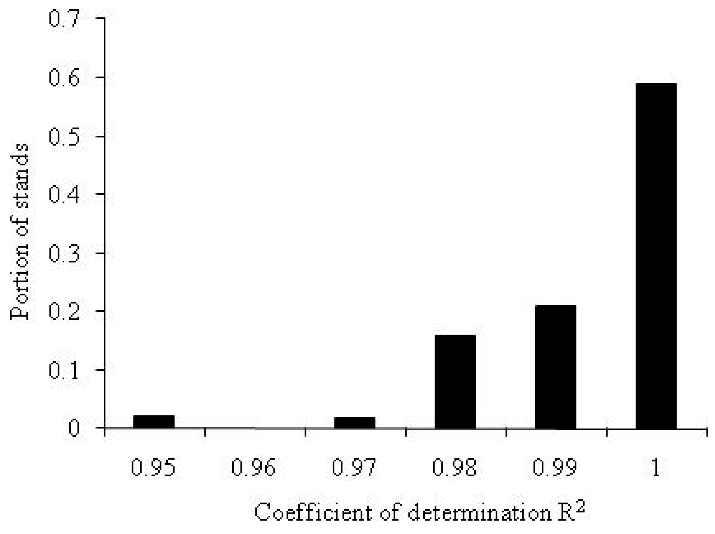
As shown in Figure 2A, for 97% of the datasets on the distribution of phytomass among tree components analyzed here, the value of the coefficient of determination of the rank distribution equation is higher than R2 = 0.98. Thus, the theoretical Equation (A2) is in very good agreement with the field measurement data.
Having calculated the root phytomass, one can use the data on all phytomass components of the forest stand to verify the EcoSolow model.
References
- Tjørve, E.; Tjørve, K.M.C. A unified approach to the Richards-model family for use in growth analyses: Why we need only two model forms. J. Theor. Biol. 2010, 267, 417–425. [Google Scholar] [CrossRef] [PubMed]
- Tsoularis, A.; Wallace, J. Analysis of logistic growth models. Math. Biosci. 2002, 179, 21–55. [Google Scholar] [CrossRef]
- Khamanis, A.; Ismail, Z.; Haron, K.; Mohammed, A.T. Nonlinear growth models for modeling oil palm yield growth. J. Math. Stat. 2005, 1, 225–233. [Google Scholar]
- Skene, K.R. The energetics of ecological succession: A logistic model of entropic output. Ecol. Model. 2013, 250, 287–293. [Google Scholar] [CrossRef]
- Aspinall, R.J. Use of logistic regression for validation of maps of the spatial distribution of vegetation species derived from high spatial resolution hyperspectral remotely sensed data. Ecol. Model. 2002, 157, 301–312. [Google Scholar] [CrossRef]
- Kumar, R.; Nandy, S.; Agarwal, R.; Kushwaha, S.P.S. Forest cover dynamics analysis and prediction modeling using logistic regression model. Ecol. Indic. 2014, 45, 444–455. [Google Scholar] [CrossRef]
- Koralewski, T.E.; Wang, H.H.; Grant, W.E.; Byram, T.D. Plants on the move: Assisted migration of forest trees in the face of climate change. For. Ecol. Manag. 2015, 344, 30–37. [Google Scholar] [CrossRef]
- Acevedoa, M.A.; Marcanob, M.; Fletcher, R.J., Jr. A diffusive logistic growth model to describe forest recovery. Ecol. Model. 2012, 244, 13–19. [Google Scholar] [CrossRef]
- Odum, H.T. Systems Ecology: An Introduction; Wiley: New York, NY, USA, 1983; p. 644. [Google Scholar]
- Usoltsev, V.A. Phytomass of the Forests in North Eurasia: Database and Geography; Ural Branch of the Russian Academy of Sciences: Ekaterinburg, Russia, 2001; pp. 183–702. (In Russian) [Google Scholar]
- Usoltsev, V.A. Fitomassa i Pervichnaya Produktsiya Lesov Evrazii (Phytomass and Primary Production of Eurasian Forests); Ural Branch of the Russian Academy of Sciences: Yekaterinburg, Russia, 2010; pp. 18–512. (In Russian) [Google Scholar]
- Clark, D.A.; Brown, S.; Kicklighter, D.W.; Chambers, J.Q.; Thomlinson, J.R.; Ni, J. Measuring net primary production in forests: concepts and field methods. Ecol. Appl. 2001, 11, 356–370. [Google Scholar] [CrossRef]
- Kloeppel, B.D.; Harmon, M.E.; Fahey, T.J. Estimating aboveground net primary productivity in forest-dominated ecosystems. In Principles and Standards for Measuring Primary Production; Fahey, T.J., Knapp, A.K., Eds.; Oxford University Press: New York, NY, USA, 2007; pp. 63–81. [Google Scholar]
- Sala, O.E.; Biondini, M.E.; Lauenroth, W.K. Bias in estimates of primary production: An analytical solution. Ecol. Model. 1988, 44, 43–55. [Google Scholar] [CrossRef]
- Waring, R.H.; Landsberg, J.J.; Williams, M. Net primary production of forests: A constant fraction of gross primary production? Tree Physiol. 1998, 18, 129–134. [Google Scholar] [CrossRef] [PubMed]
- Meng, S.; Jia, Q.; Zhou, G.; Zhou, H.; Lui, Q.; Yu, J. Fine Root Biomass and Its Relationship with Aboveground Traits of Larix gmelinii Trees in Northeastern China. Forests 2018, 9, 35. [Google Scholar] [CrossRef]
- Wang, B.; Li, M.; Fan, W.; Yu, Y.; Chen, J.M. Relationship between Net Primary Productivity and Forest Stand Age under Different Site Conditions and Its Implications for Regional Carbon Cycle Study. Forests 2018, 9, 5. [Google Scholar] [CrossRef]
- Sisay, K.; Thurnher, C.; Belay, B.; Lindner, G.; Hasenauer, H. Volume and Carbon Estimates for the Forest Area of the Amhara Region in Northwestern Ethiopia. Forests 2017, 8, 122. [Google Scholar] [CrossRef]
- Kolchugina, T.P.; Vinson, T.S. Equilibrium analysis of carbon pools and fluxes of forest biomes in the former Soviet Union. Can. J. For. Res. 1993, 23, 81–88. [Google Scholar] [CrossRef]
- Shvidenko, A.; Schepschenko, D.; Nilsson, S.; Bouloui, Y. Semi-empirical models for assessing biological productivity of Northern Eurasian forests. Ecol. Model. 2007, 204, 163–179. [Google Scholar] [CrossRef]
- Shvidenko, A.; Schepaschenko, D.; McCallum, I.; Nilsson, S. Can the uncertainty of full carbon accounting of forest ecosystems be made acceptable to policymakers? Clim. Chang. 2010, 103, 137–157. [Google Scholar] [CrossRef]
- Solow, R.M. A Contribution to the Theory of Economic Growth. Q. J. Econ. 1956, 70, 65–94. [Google Scholar] [CrossRef]
- Houthakker, H.S. The Pareto Distribution and the Cobb–Douglas Production Function in Activity Analysis. Rev. Econ. Stud. 1955, 23, 27–31. [Google Scholar] [CrossRef]
- Cobb, C.W.; Douglas, P.H. A Theory of Production. Am. Econ. Rev. 1928, 18, 139–165. [Google Scholar]
- Jesus, F.; Gerard, A.F. The Estimation of the Cobb-Douglas Function: A Retrospective View. East. Econ. J. 2005, 31, 427–445. [Google Scholar]
- Jackson, R.B.; Canadell, J.; Ehleringer, J.R.; Mooney, H.A.; Sala, O.E.; Schulze, E.D. A global analysis of root distributions for terrestrial biomes. Oecologia 1996, 108, 389–411. [Google Scholar] [CrossRef] [PubMed]
- Vogt, K.A.; Vogt, D.J.; Bloomfield, J. Analysis of some direct and indirect methods for estimating root biomass and production of forests at an ecosystem level. Plant Soil 1998, 200, 71–89. [Google Scholar] [CrossRef]
- Chen, W.; Zhang, Q.; Cihlar, J.; Bauhus, J.; Price, D.T. Estimating fine-root biomass and production of boreal and cool temperate forests using aboveground measurements: A new approach. Plant Soil 2004, 265, 31–46. [Google Scholar] [CrossRef]
- Curt, T.; Lucot, E.; Bouchaud, M. Douglas-fir root biomass and rooting profile in relation to soils in a mid-elevation area (Beaujolais Mounts, France). Plant Soil 2001, 233, 109–125. [Google Scholar] [CrossRef]
- Li, Z.; Kurz, W.A.; Apps, M.J.; Beukema, S.J. Belowground biomass dynamics in the carbon budget model of the Canadian forest sector: Recent improvements and implications for the estimation of NPP and NEP. Can. J. For. Res. 2003, 33, 126–136. [Google Scholar] [CrossRef]
- Sukhovolsky, V.G. Free competition of tree parts for resources and allometric correlations. J. Gen. Biol. 1997, 5, 80–88. (In Russian) [Google Scholar]
- Soukhovolsky, V.G.; Ivanova, J.D. Estimation of Forest Stand Net Primary Productivity Using Fraction Phytomass Distribution Model. Contemp. Probl. Ecol. 2013, 6, 700–707. [Google Scholar] [CrossRef]
- Ivanova, Y.; Soukhovolsky, V. Net primary production in forest ecosystem of middle siberia: Assessment using a model of tree component phytomass distribution. In Climate Change Impacts on High-Altitude Ecosystems; Ozturk, M., Hakeem, K.R., Faridah-Hanum, I., Efe, R., Eds.; Springer International Publishing: Basel, Switzerland, 2015; pp. 627–635. [Google Scholar]
- Ferrara, M.; Guerrini, L.; Mavilia, R. Modified Neoclassical Growth Models with Delay: A Critical Survey and Perspectives. Appl. Math. Sci. 2013, 7, 4249–4257. [Google Scholar] [CrossRef]
Figure 1.
Phytomass of pine stands. (1) inventory data, Middle Siberia; (2) calculation with the ESM; (3) inventory data, South Siberia; (4) calculation with the ESM; (calculations were based on the data of different authors systematized [10,11]).

Figure 2.
Dynamics of the forest stand phytomass, including root phytomass of Larix gmelinii Rupr., Middle Siberia, (1) field data ([10], p. 589); (2) EcoSolow model calculations.
Figure 2.
Dynamics of the forest stand phytomass, including root phytomass of Larix gmelinii Rupr., Middle Siberia, (1) field data ([10], p. 589); (2) EcoSolow model calculations.

Figure 3.
NPP calculation with the balanced Equation (1), taking into account root phytomass, and with the EcoSolow Equation (2). Larix gmelinii Rupr., Middle Siberia ([10], p. 589).
Figure 3.
NPP calculation with the balanced Equation (1), taking into account root phytomass, and with the EcoSolow Equation (2). Larix gmelinii Rupr., Middle Siberia ([10], p. 589).

Figure 4.
Age dynamics of the NPP of single-species even-aged pine stands (1) South Siberia, (2) Middle Siberia).
Figure 4.
Age dynamics of the NPP of single-species even-aged pine stands (1) South Siberia, (2) Middle Siberia).

Figure 5.
Age dynamics of the NPP of forest stands in the taiga zone of Siberia [11]. (1) Larix sibirica Ledeb.; (2) Abies sibirica Ledeb.; (3) Picea obovata Ledeb.; (4) Betula pendula Rotsch.; (5) Pinus sylvestris L.
Figure 5.
Age dynamics of the NPP of forest stands in the taiga zone of Siberia [11]. (1) Larix sibirica Ledeb.; (2) Abies sibirica Ledeb.; (3) Picea obovata Ledeb.; (4) Betula pendula Rotsch.; (5) Pinus sylvestris L.

Figure 6.
Changes in the effectiveness of photosynthesis in the Scots pine trees as related to the age of the stands (1) South Siberia; (2) Middle Siberia; (3) North Siberia.
Figure 6.
Changes in the effectiveness of photosynthesis in the Scots pine trees as related to the age of the stands (1) South Siberia; (2) Middle Siberia; (3) North Siberia.
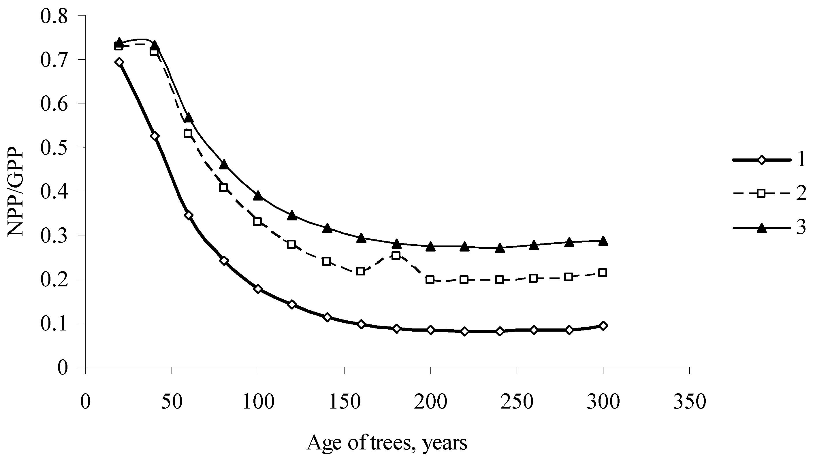
Figure 7.
The relationship between coefficients (1 − α) and s of the EcoSolow model for forest stands of different species in the northern and southern regions of Siberia. (1) in the southern regions of Siberia (Pinus sylvestris L., Larix sibirica Ledeb., Betula pendula Roth.); (2) in the northern regions of Siberia (Larix sibirica Ledeb., Abies sibirica Ledeb., Picea obovata Ledeb.).


Table 1.
Middle Siberia, south taiga.
| Age, Years | Density, Trees/ha | Phytomass, t/ha | |||
|---|---|---|---|---|---|
| Stem with Bark | Needles | Branches | Roots * | ||
| 10 | 13,522 | 7.4 | 3.13 | 2.5 | 4.3 |
| 20 | 7528 | 25.7 | 3.64 | 4.2 | 8.9 |
| 40 | 3604 | 61.2 | 3.8 | 6.2 | 14.9 |
| 60 | 2167 | 85.4 | 3.71 | 7.4 | 18.0 |
| 80 | 1477 | 100.2 | 3.56 | 8.1 | 19.6 |
| 100 | 1075 | 108.3 | 3.41 | 8.6 | 20.4 |
| 120 | 827 | 113.1 | 3.27 | 8.9 | 20.8 |
| 140 | 656 | 114.4 | 3.13 | 9.1 | 20.8 |
| 160 | 542 | 113.8 | 3.0 | 9.2 | 20.6 |
| 180 | 453 | 112.6 | 2.89 | 9.3 | 20.4 |
| 200 | 382 | 110.7 | 2.78 | 9.4 | 20.1 |
| 220 | 331 | 107.7 | 2.68 | 9.4 | 19.7 |
| 240 | 289 | 104.5 | 2.59 | 9.4 | 19.2 |
| 260 | 255 | 101.5 | 2.51 | 9.4 | 18.7 |
| 280 | 226 | 97.8 | 2.42 | 9.3 | 18.3 |
| 300 | 202 | 94.7 | 2.35 | 9.3 | 17.9 |
* Estimated—Appendix A.
| Woody Species, Location | ESM Parameters | ||
|---|---|---|---|
| A | α | s | |
| Pinus sylvestris L., 53°50′ N 92° E | 0.72 | 0.23 | 0.54 |
| Pinus sylvestris L., 51°45′ N 94°30′ E | 0.56 | 0.27 | 0.50 |
| Larix sibirica Ledeb., 54° N, 91°E | 1.60 | 0.09 | 0.23 |
| Larix sibirica Ledeb., 52° N, 95°30′ E | 1.39 | 0.17 | 0.70 |
| Picea obovata Ledeb., 56°35′ N, 57°40′ E | 1.10 | 0.11 | 0.70 |
| Picea obovata Ledeb., 59° N, 61° E | 0.73 | 0.28 | 0.39 |
| Abies sibirica Ledeb., 59° N, 93° E | 0.67 | 0.24 | 0.28 |
| Betula pendula Roth., 57° N, 93° E | 2.03 | 0.33 | 0.94 |
| Betula pendula Roth., 55°10′ N, 92° E | 1.83 | 0.31 | 0.67 |
| Pinus sylvestris L., 59°30′ N, 101°50′ E | 0.61 | 0.25 | 0.50 |
© 2018 by the authors. Licensee MDPI, Basel, Switzerland. This article is an open access article distributed under the terms and conditions of the Creative Commons Attribution (CC BY) license (http://creativecommons.org/licenses/by/4.0/).
Share and Cite
MDPI and ACS Style
Soukhovolsky, V.; Ivanova, Y. Modeling Production Processes in Forest Stands: An Adaptation of the Solow Growth Model. Forests 2018, 9, 391. https://doi.org/10.3390/f9070391
AMA Style
Soukhovolsky V, Ivanova Y. Modeling Production Processes in Forest Stands: An Adaptation of the Solow Growth Model. Forests. 2018; 9(7):391. https://doi.org/10.3390/f9070391
Chicago/Turabian StyleSoukhovolsky, Vlad, and Yulia Ivanova. 2018. "Modeling Production Processes in Forest Stands: An Adaptation of the Solow Growth Model" Forests 9, no. 7: 391. https://doi.org/10.3390/f9070391
Note that from the first issue of 2016, this journal uses article numbers instead of page numbers. See further details here.