Short-Term Vegetation Responses Following Windthrow Disturbance on Preserved Forest Lands

Abstract

Invasive exotic plants pose a serious threat to the ecological integrity of forests in the eastern United States. Presence and expansion of these plants are closely associated with human-caused disturbances. Land preservation to exclude human-caused disturbances could protect against invasions, yet natural disturbances persist. We ask if windthrow forest disturbances in preserved National Park lands facilitate exotic species invasions. We hypothesized that exotic plant expansion is positively correlated with forest canopy disturbance from windthrow and proximity of disturbed area to forest edge. Pre and post-disturbance data from National Park Service long-term vegetation monitoring were used to analyze exotic plant richness and abundance in four National Park Service units affected by 2012 severe storms. No significant difference in exotic plant richness or cover occurred between disturbed (n = 18) and undisturbed plots (n = 262) over three years following disturbance. Exotic plant cover prior to disturbance was positively correlated with the amount of nearby linear edge habitat, but there were no significant correlations between edge and change in exotic plant cover following disturbance. Lack of increase in exotic plants after windthrow disturbance suggests that land preservation provides short-term resistance to invasion.

1. Introduction

Land preservation, a key strategy of conservation biology, is the effort to protect habitat from human-caused impacts such as fragmentation, development, species loss, and the encroachment of invasive exotic plants [1,2]. The establishment and range expansion of exotic plants are closely associated with human disturbances such as logging, mining, road construction, agriculture, horticulture, and development [3,4,5]. This link between exotic plants and anthropogenic disturbance is the result of both direct and indirect effects. Not only are humans often responsible for the disturbances that facilitate exotic plant invasion, they often are directly responsible for the dispersal of exotic plants into these areas through propagule transport [2,6,7]. Invasive exotic plants tend to be pioneer species with high reproductive rates and effective propagule dispersal mechanisms [8], traits amenable to colonizing newly disturbed areas [9]. Disturbed areas tend to harbor exotic plants and can act as propagule sources [3,10,11]. As a result, contiguously forested areas near disturbed habitats are more likely to become invaded than interior forests [12]. Even within preserved lands, roads and private lands can be pervasive, creating a patchwork of edge habitat (e.g., roads, fields, recent logging, and developments). Forest roads in particular are important vectors for the spread of invasive exotic plants [11,13]. This link between anthropogenic disturbance and exotic plants has justified setting aside large tracts of land to maintain ecological integrity [14,15]. However, despite efforts to limit anthropogenic disturbance, natural disturbances such as tree canopy windthrow, fire, and flooding continue unabated. Given natural disturbances will continue unabated: Is removal of human disturbances through land preservation effective in limiting exotic plants?

Invasive exotic plants pose a serious threat to native ecosystems through mechanisms such as competition, allelopathy, and habitat manipulation [16,17,18]. Exotic plants can outcompete and displace native plants, as is the case for species such as tree-of-heaven (Ailanthus altissima (Mill.) Swingle) and Japanese stiltgrass (Microstegium vimineum (Trin.) A. Camus) [11,19]. Furthermore, exotic plants may decrease biodiversity, which can have cascading impacts across species and trophic levels [20,21,22,23]. Invasion can disrupt ecological communities and may limit native tree re-establishment following a disturbance [24,25]. Given the tendency of invasive plants to take advantage of available resources, disturbed areas present a prime opportunity for invasive plants to exploit.

Canopy disturbances in forests tend to increase the amount of sunlight reaching the forest floor, promoting new plant growth and forest heterogeneity through variable forest structure and new species composition [5,15,26]. Canopy disturbances have the potential to affect all forests; however, forests without a preservation mandate are commonly salvage logged following natural disturbance events [27]. Salvage logging increases exotic plant abundance due to more light reaching the forest floor, along with more exposed soil [26,27]. Preserved lands on the other hand present an opportunity to observe whether exotic plants opportunistically invade following natural disturbance despite the absence of anthropogenic disturbance.

In this study we focus on two natural disturbance events, severe storm systems Hurricane Sandy and a wind event known as the 29 June Derecho, which impacted the Central Appalachians in 2012 and caused a patchwork of tree windthrow and canopy gaps. These events generated a prime opportunity to investigate species responses to forest canopy disturbances in preserved lands. We used data from National Park Service (NPS) long-term vegetation monitoring plots [28], located in areas affected by storm windthrow, to answer the following two questions. First, in preserved lands, does natural disturbance facilitate exotic vascular plant species invasion? We compared vegetation measured in plots before and after the 2012 forest canopy windthrow from severe storms to quantify changes in species richness and cover as a result of natural disturbance. We hypothesized that canopy disturbance and exotic plant colonization were positively correlated. Secondly, does proximity to edge habitat increase the abundance of exotic plants in naturally disturbed preserved areas? To address this question, we studied the interaction between plot proximity to edge habitat and plant species composition in disturbed and undisturbed areas. We hypothesized that canopy gaps with more adjacent edge habitats would have greater exotic plant cover pre-disturbance and a proportionally greater increase in these plants post-disturbance correlating to the amount of edge.

2. Materials and Methods

2.1. Study Areas

The study areas were located in four United States National Park Service (NPS) units in the Central Appalachian Mountains: Bluestone National Scenic River (BLUE) in West Virginia (WV), Delaware Water Gap National Recreation Area (DEWA) in Pennsylvania (PA) and New Jersey (NJ), Gauley River National Recreation Area (GARI) in WV, and New River Gorge National River (NERI) in WV. The dominant forest types included dry oak-hickory-heath and mesic sugar maple-beech-basswood forests, though these parks cover a wide range of vegetation types, land-use histories, and baseline exotic plant prevalence [29,30,31,32]. DEWA, located along the Delaware River, has had longer and more intensive agricultural use than the other NPS units, as well as having a much greater human population density both historically (post-European colonization) and currently. These factors have led to a higher proportion of exotic plants in DEWA compared to the NPS units in West Virginia [33].

These four NPS units contain 282 long-term vegetation monitoring plots that were established to monitor the long-term health of these forests and are intended to be sampled in perpetuity. The intensive sampling design prevents all 282 plots from being sampled in one growing season, and, therefore, the plots are sampled on a rotating panel design over a four-year period with one quarter of all plots sampled each year between 2007 and 2010, and resampled between 2011 and 2014 with a third round of sampling beginning in 2015 [28]. A detailed justification of the sampling design and data collection methods can be found in Perles et al. 2014a [28]. Here we only present an overview of the sampling methods. Protocols from the US Forest Service’s Forest Inventory Analysis program [34] and four NPS Inventory and Monitoring protocols from networks in the eastern U.S. were fundamental in establishing these methods [35,36,37,38].

Monitoring plots were selected from a regular grid of possible sampling points using a Generalized Random-Tessellation Stratified design [39] to ensure a balanced sample while still maintaining a random design. Points that fell on managed lands (i.e., parking lots, lawns, roads, etc.) were removed, as were sites that had >30 degree slope. Selected plot locations were installed and sampled in a four-year rotating panel design, meaning that a quarter of the total plots were installed each year from 2007 to 2010 and resampled between 2011 and 2014 with a third round of sampling beginning in 2015. All plots were resampled within two weeks of the date of original installation to capture a similar suite of the flora present at that time of year.

In October 2012 Hurricane Sandy brought high winds, heavy rains, and flooding to parts of the Mid-Atlantic including DEWA, while the 2012 Derecho (June 2012) swept across the upper Mid-West and Mid-Atlantic including BLUE, GARI, and NERI. A total of 18 plots (6.3% of all plots) were disturbed by these storms, one in BLUE, five in DEWA, seven in GARI, and five in NERI.

2.2. Field Methods

Plots were comprised of a 15-m radius circle, within which an array of forest condition measurements were sampled including live tree basal area (LBA), coarse woody debris (CWD), and vascular understory plant richness and cover. Plots were marked with metal spikes to ensure that the same areas were sampled each visit. A center point marked with rebar and a metal cap was installed, along with 25 cm galvanized metal nails that mark the ends of transects along the 0, 60, 120, 180, 240, and 300 degree azimuths from plot center.

Along the six transects, 12 1 m × 1 m quadrats were sampled to capture cover of all vascular plants by species covering an area under 2 m in height. In each quadrat, each species was given a cover class (0%, 1–2%, 2–5%, 5–10%, 10–25%, 25–50%, 50–75%, 75–95%, and 95–100%), and the midpoints of these cover classes were used in the analysis to represent species cover. The midpoint value of each cover class represents the mean of the two values at each end of each range. The average total cover of all species for a plot was calculated by summing the cover midpoints from all species within each quadrat and then averaging the summed values across the 12 quadrats. Total cover for a quadrat or average total cover for a plot may exceed 100% (or 1 m²) due to overlap of species canopies. Average species richness for each plot was calculated by determining species richness in each quadrat and then averaging those values across the 12 quadrats.

All plant taxa were classified as native or exotic and those designations were used to calculate native and exotic cover and richness using the formulas described above. Invasive exotic species can be difficult to define, let alone classify into a system to rank invasiveness. Therefore, we did not differentiate the degree of invasiveness between the different species and pooled exotic species in order to simplify the study. However, nearly all of the exotic plant species found in the disturbed plots are considered moderately or highly invasive according to NatureServe’s Invasive Species Impact Rank (I-Rank) classification system (Appendix A,

Table A8. List of exotic plants by NPS unit with their U.S. Invasive Species Impact Rank (I-Rank). This table shows all of the exotic plants present in the quadrats of the disturbed plots. I-Rank is a ranking system established by NatureServe, The Nature Conservancy, and the NPS, which assesses exotic plants within the U.S. to determine which species may have the most detrimental impacts to native species and ecosystems. Not all species have been assessed for level of invasiveness. Unassessed species are ranked “N/A.” (For more information see http://explorer.natureserve.org/impact_rank.htm).

NPS Unit	Species (Scientific Name)	Taxonomic Authority	Species (Common Name)	I-Rank
BLUE	Lonicera japonica	Thunb.	Japanese honeysuckle	High/Medium
BLUE	Rubus phoenicolasius	Maxim.	Wineberry	Medium
DEWA	Alliaria petiolata	(M. Beib) Cavara and Grande	Garlic mustard	High/Medium
DEWA	Berberis thunbergii	DC.	Japanese barberry	High/Medium
DEWA	Cardamine impatiens	L.	Narrowleaf bittercress	Low
DEWA	Celastrus orbiculatus	Thunb.	Oriental bittersweet	High/Medium
DEWA	Elaeagnus umbellata	Thunb.	Autumn-olive	High
DEWA	Hesperis matronalis	L.	Dame’s rocket	Medium/Low
DEWA	Lonicera morrowii	A. Gray	Morrow’s honeysuckle	High/Medium
DEWA	Microstegium vimineum	(Trin.) Camus	Japanese stiltgrass	High/Medium
DEWA	Polygonum caespitosum	Blume	Oriental lady’s thumb	N/A
DEWA	Rhamnus cathartica	L.	European buckthorn	High/Medium
DEWA	Rosa multiflora	Thunb.	Multiflora rose	Medium/Low
DEWA	Rubus phoenicolasius	Maxim.	Wineberry	Medium
GARI	Ailanthus altissima	(Mill.) Swingle	Tree-of-heaven	Medium
GARI	Microstegium vimineum	(Trin.) Camus	Japanese stiltgrass	High/Medium
NERI	Ailanthus altissima	(Mill.) Swingle	Tree-of-heaven	Medium
NERI	Alliaria petiolata	(M. Beib) Cavara and Grande	Garlic mustard	High/Medium
NERI	Cardamine impatiens	L.	Narrowleaf bittercress	Low
NERI	Glechoma hederacea	L.	Creeping charlie	Low
NERI	Lonicera morrowii	A. Gray	Morrow’s honeysuckle	High/Medium
NERI	Polygonum persicaria	L.	Spotted lady’s thumb	N/A
NERI	Rosa multiflora	Thunb.	Multiflora rose	Medium/Low

), which provides some context for the invasiveness of the exotic plants encountered in this study. An I-Rank protocol was developed to rank invasive exotic plant species primarily by their detrimental impact to biodiversity [40].

CWD was sampled along the six transects for fallen wood greater than 7.5 cm in diameter at its intersection with each transect. Huber’s formula [41] was used to estimate CWD volume from line intersect transect data using the diameter of each CWD piece measured at the point of intersection with the transect line [42]. This calculation was slope-corrected by converting the slope-length of each line intersect transect to its equivalent horizontal distance [43]. Inserting a correction factor into the formula allows calculation of CWD volume per hectare (m³∙ha⁻¹) as

$$CWD=CWD=\frac{{\pi }^2\sqrt{1+{\left(\frac{\% Slope}{100}\right)}^2}}{8\times Slope\_length}\times {\sum }_i^{n}Dia{m}_i^2$$

where %Slope is percent slope of the transect, Slope_length is the slope length of the transect in meters (i.e., 15 m), and Diam_i is the recorded diameter in centimeters of each piece of coarse woody debris. CWD volume was then averaged across the six transects to generate average CWD volume per plot, expressed as a volume (m³∙ha⁻¹).

Trees were measured for diameter at breast height (dbh) in cm, which is 1.37 m from the base of the tree on the uphill side, and scribed 5 cm below dbh to ensure precise measurements between sampling periods. Trees greater than 10 cm at dbh and within 15 m horizontal distance of the plot center were sampled. DEWA had five undisturbed plots without any trees present and those plots were excluded from the analyses because there were no trees that could have been blown over. Live tree basal area in square meters was calculated from dbh (cm) using the following formula below. Plot live basal area was calculated as the sum of the basal area of all the live trees in that plot. This value was converted to m²∙ha⁻¹ by dividing by the plot area (707 m²) and converting to hectares:

$$\mathrm{LBA}={{\displaystyle \sum }}_i^n\left[\pi \times {\left(\frac{dbh}{2\times 100}\right)}^2\right]\times \left(\frac{\mathrm{10,000}}{707}\right)$$

2.3. Disturbance Criteria

Plots were identified as disturbed if they experienced windstorm disturbance damage (i.e., stem breakage or tip-up) since the time of last sampling to >25% of all trees in a plot, or a disturbance (i.e., trees and tree tops falling into a plot) to >25% of the soil surface, understory vegetation, or canopy trees. These thresholds were coarse measurements designed to record disturbances that may have influenced the plot structure.

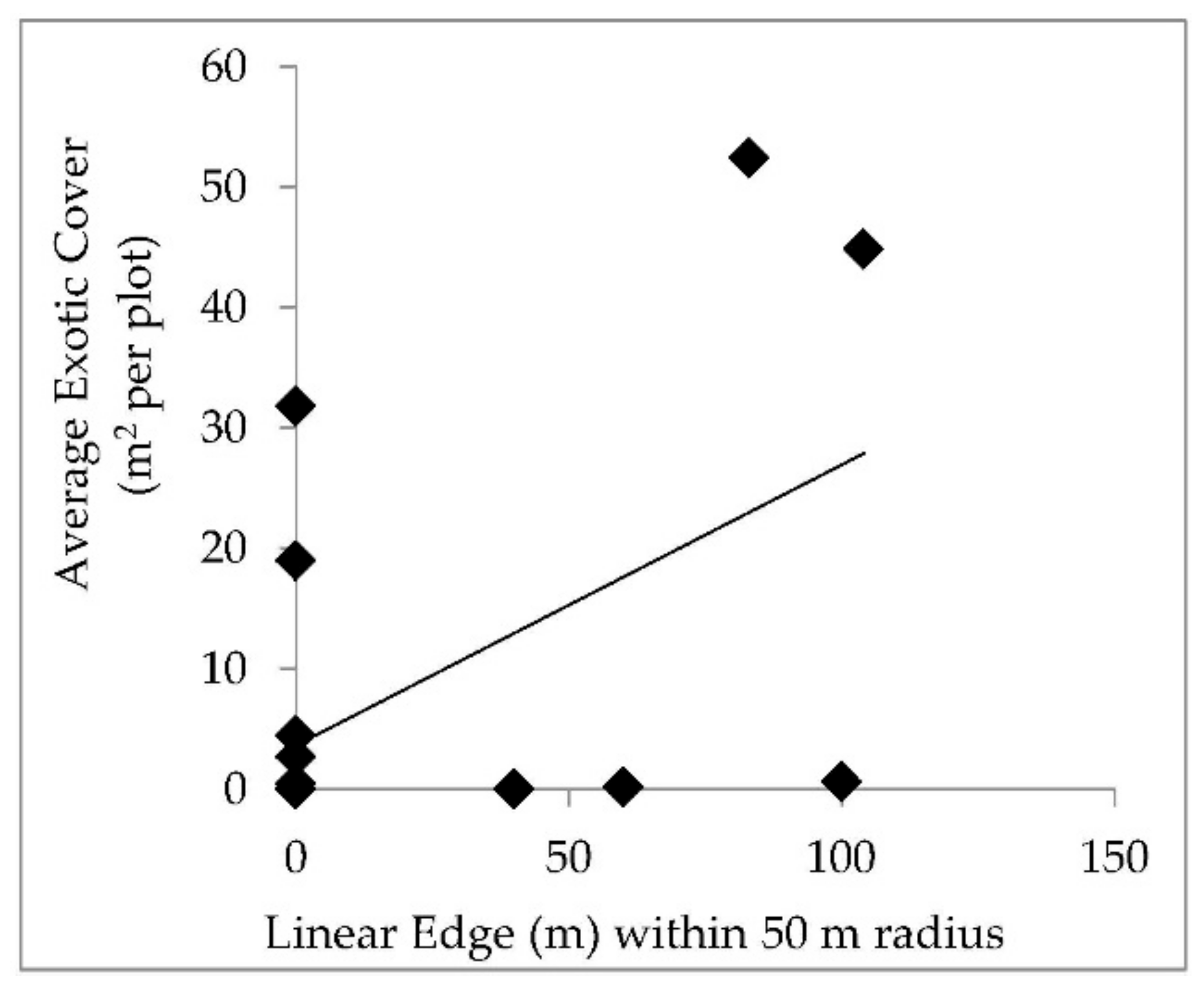
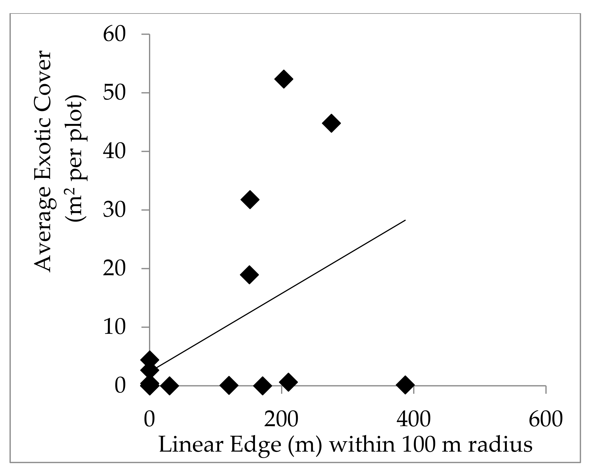
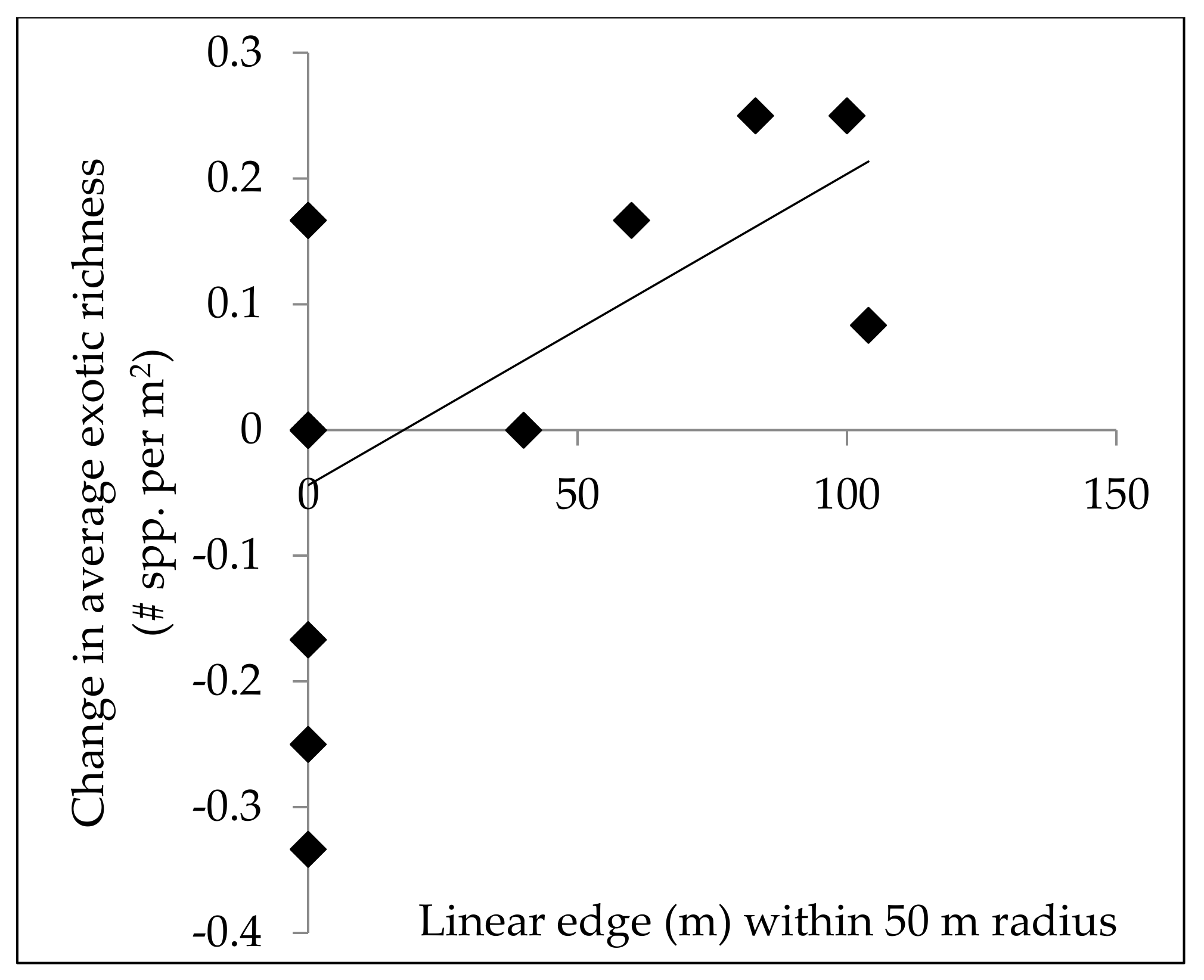
Edge habitat is ideal for invasive exotic plants due to high light availability, and can act as a source of propagule pressure for the surrounding area, so we quantified the amount of edge habitat for disturbed plots to relate to invasive exotic plant richness and abundance. The amount of linear edge surrounding each disturbed plot was measured using Google Earth Pro’s “Ruler” tool. Linear edge was defined as the edges of roads, fields, and other human developments. Measurements of total linear edge within 50 m, 100 m, and 250 m of the plot center were recorded. These distances were chosen based on research from Mortensen et al. 2009 [11]. To determine if roads had a distinct impact on exotic plant recruitment in plots, the edge habitat along roads was analyzed separately, as well as grouped with other sources of edge habitat.

2.4. Data Analyses

Vegetation monitoring data from the NPS were used to study forest changes following disturbance. These data are made publicly available here: https://irma.nps.gov/DataStore/. Data prior to disturbance from disturbed and undisturbed plots were compared to establish if disturbed plots were representative of NPS unit conditions. The amount of linear edge habitat to exotic plant cover and richness in plots that were later disturbed was compared to determine if edge habitat was associated with exotic plant abundance.

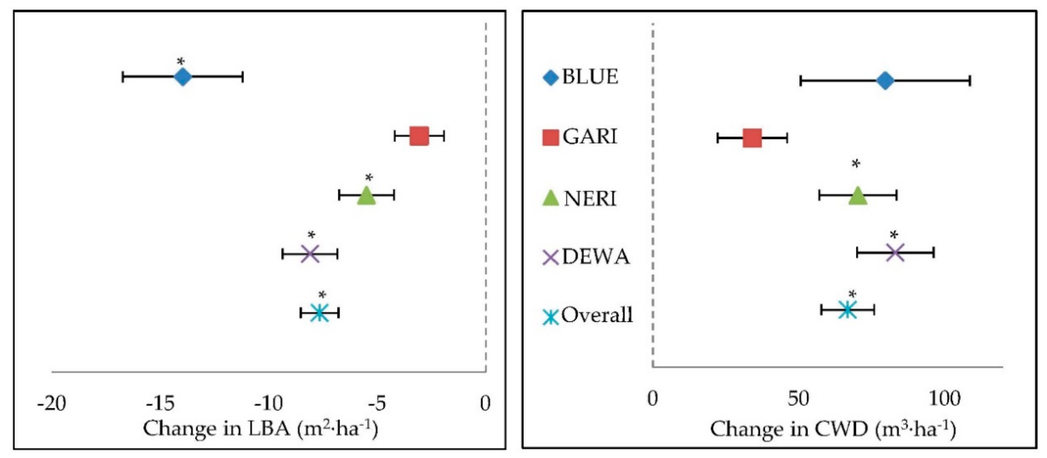
Vegetation responses to disturbance were compared by assessing post-disturbance forest structure (LBA and CWD) in disturbed versus undisturbed plots to confirm that disturbance impacted disturbed plots. Changes in plant species richness and cover in disturbed plots were compared from pre- to post-disturbance sampling; amount of linear edge habitat was then compared to these changes to determine if edge habitat was associated with exotic plant colonization.

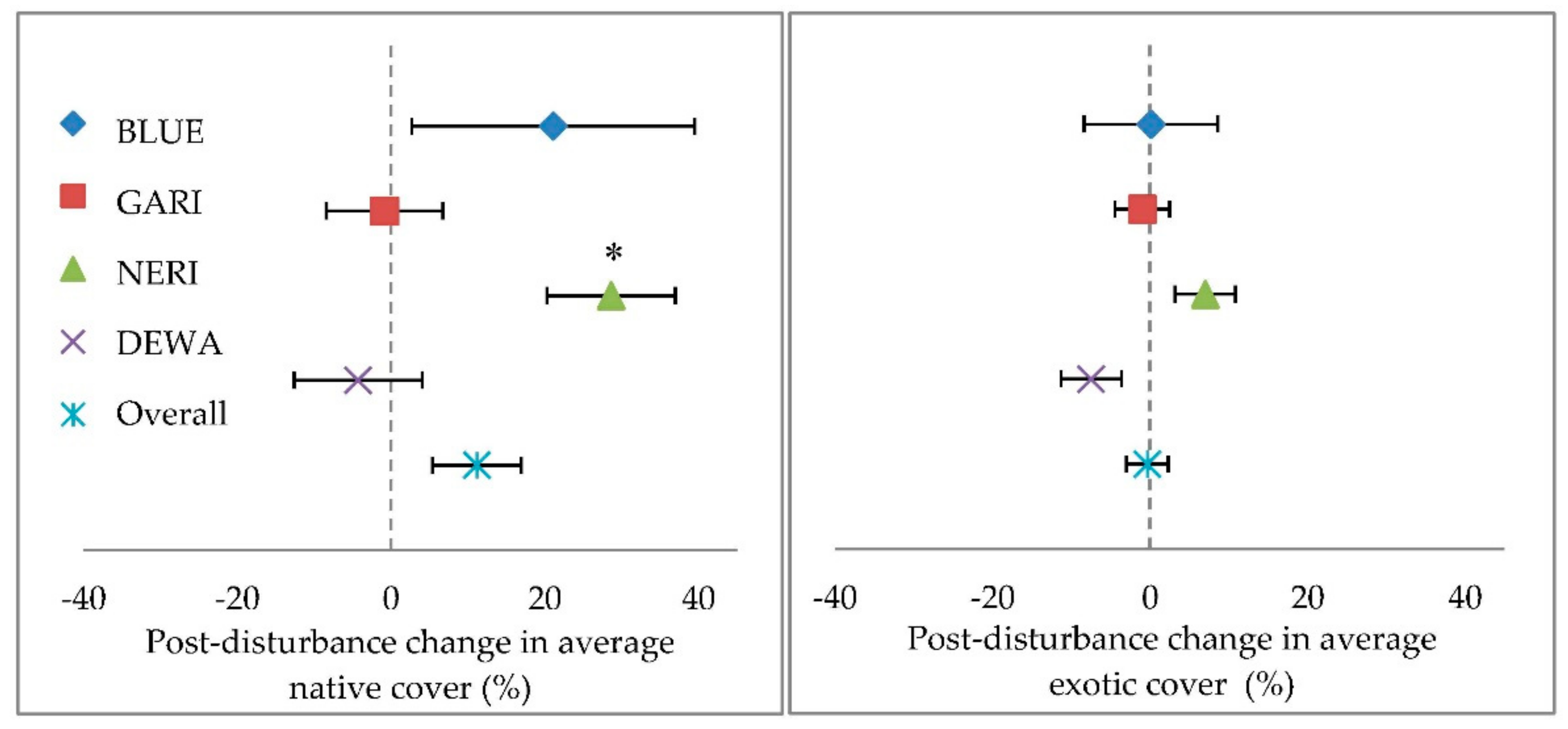
The statistical programs Minitab and Microsoft Excel were used to analyze LBA, CWD, plant species richness, plant cover, and edge habitat data. Tukey’s method was used to calculate differences of means for LBA, CWD, and native and exotic plant richness. Native and exotic plant cover were analyzed using a general linear mixed model ANOVA in Minitab. NPS unit, plot condition (disturbed or undisturbed), and disturbance event (pre- or post-disturbance) were fixed factors in the ANOVA and interactions between NPS unit and plot condition, NPS unit and disturbance events, and plot condition and disturbance events were added into the model. Significant differences of means between LBA, CWD, native and exotic plant richness, as well as native and exotic plant cover, were identified at a = 0.05.

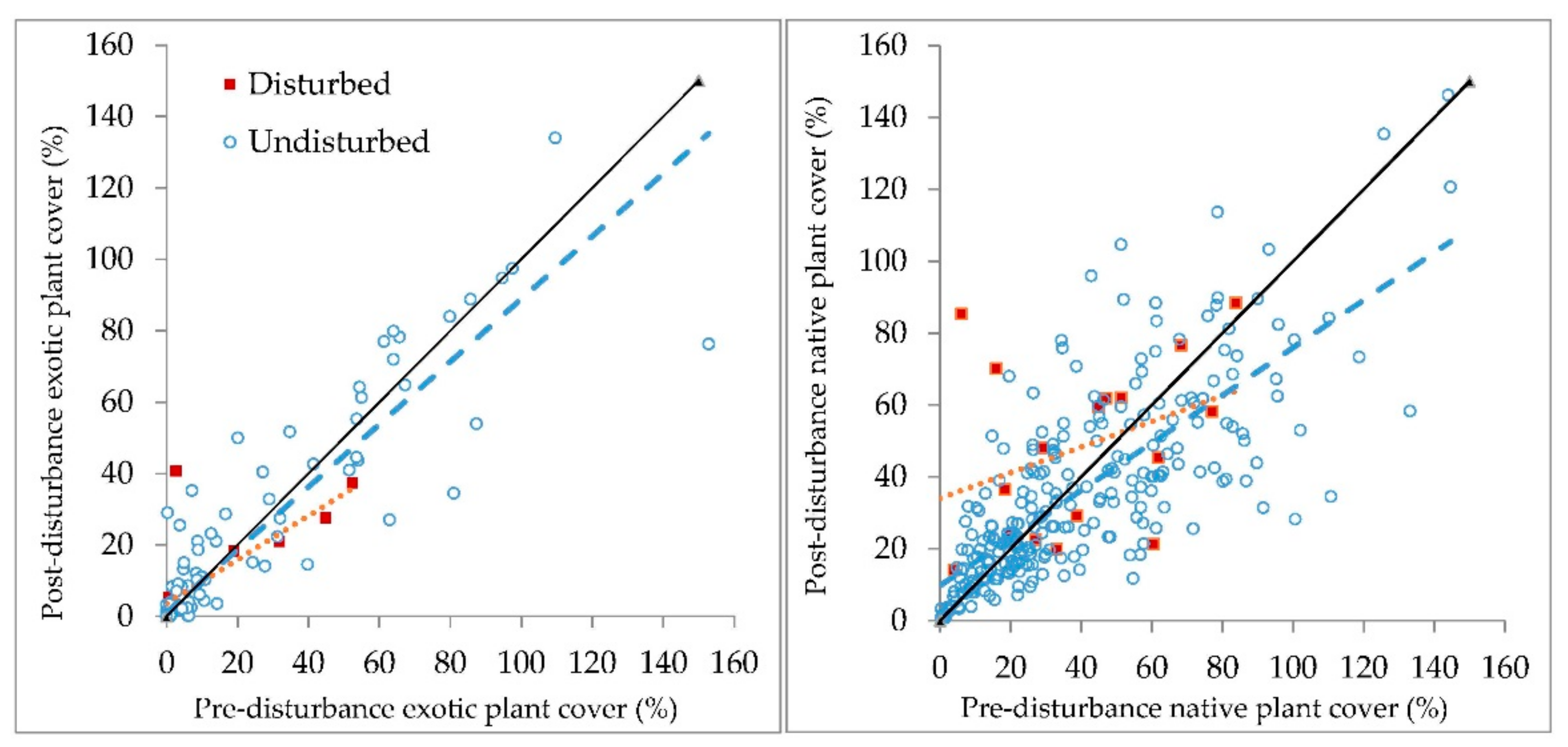
Amount of linear edge was compared by linear regression to plant cover and richness prior to disturbance and to the changes in plant cover (post-disturbance minus pre-disturbance) and richness for disturbed plots. Pre- and post-disturbance plant cover in disturbed and undisturbed plots were compared by linear regression, and the slope of those lines compared to the equation y = x that represents no change in cover or richness from pre- to post-disturbance.

2.5. Limitations

This study used data from an NPS long-term vegetation monitoring program that were not originally designed to capture in-depth details about the impacts of natural and stochastic disturbance events. However, pre-disturbance forest vegetation data from these plots presented a unique and exciting opportunity to investigate the impacts of these storms. The opportunistic nature of the study leads to particular limitations. For example, the monitoring protocol allowed for a coarse identification of canopy disturbance and does not capture gap size, which would be a better metric for the study of vegetation response to natural canopy disturbance. In addition, disturbance impacts would ideally be compared between disturbed and control plots, however we were unable to identify control plots that matched disturbed plots in all ways except disturbance, therefore we compared the 18 disturbed plots to the population of 262 monitoring plots. The limited number of disturbed plots should also be considered in the interpretation of results. Post-disturbance sampling happened over four field seasons following the 2012 storms. We did not separate plots by the time relative to disturbance because the number of plots in each time period varied widely. Plots were sampled from <1 to 3 years following disturbance, but one year had as many as ten disturbed plots while another year only had one disturbed plot. Years since disturbance was initially included as a covariate for most analyses, however it was removed in the final models because it explained little of the model variation. Ultimately, the time between the disturbance events and plot sampling was relatively short (<3 years). These findings only offer a view into initial vegetation responses and further work exploring long-term changes would certainly help demonstrate if these trends continue as the canopy re-establishes overtime. Finally, the inventory protocol uses a two-dimensional estimate of percent cover by species, which could be highly influenced by coarse woody debris dropping from the canopy from the wind disturbance.

3. Results

3.1. Pre-Disturbance Comparisons

Prior to the 2012 canopy disturbance events, average plot CWD volume in BLUE, NERI, and DEWA did not differ significantly between the disturbed and undisturbed plots, whereas GARI disturbed plots had significantly more CWD than the remaining park plots prior to the disturbance event (Figure S1, Table S1). This higher pre-disturbance CWD volume in GARI disturbed plots is likely due to the older forests found within that park unit [33]. Pre-disturbance LBA was also higher in the GARI disturbed plots compared to the undisturbed plots (Table S1). Higher CWD and LBA in disturbed plots prior to disturbance at GARI suggests that these plots could have been more susceptible to disturbance, whether due to larger trees or perhaps loss of wind protection for trees adjacent to the canopy gaps that produced the CWD. In BLUE, GARI, and NERI, average LBA of the disturbed plots prior to disturbance were not significantly different from the undisturbed plots (Figure S1). The LBAs of disturbed plots in DEWA were significantly higher prior to the disturbance events because many of the undisturbed plots in DEWA were located on early successional abandoned agricultural fields with extremely low LBA (Figure S1). These early successional systems were not susceptible to wind disturbance effects because there were very few trees.

Prior to disturbance, no NPS unit had significant differences between the disturbed and undisturbed plots in average native or exotic plant cover or species richness (Figures S2 and S3). Overall, the pre-disturbance exotic plant cover and richness for disturbed plots was highly variable. Species richness was roughly 13 times greater for native plants compared to exotic plants (Table S2).

Prior to disturbance, edge habitat may have generally aided the expansion of exotic plants into these forests because the linear edge of forest within 50 and 100 m radii of the plots was positively correlated with average total cover of exotic plants (y = 0.23x + 3.69, p-value = 0.022, and R² = 0.28, y = 0.07x + 2.38, p-value = 0.042, and R² = 0.22, respectively; Appendix A and Figure A1 and Figure A2). The linear edge within 250 m radii around plots was not significantly correlated with average total cover of exotic plants (y = 0.01x + 0.81, p-value = 0.15, and R² = 0.13), suggesting propagule pressure declines relative to distance from edge habitat. Average exotic plant richness prior to disturbance was not correlated to amount of linear edge within 50, 100, or 250 m from plot centers (y = 0.397 + 0.01x and p-value = 0.07, y= 0.299 + 0.004x and p-value = 0.07, and y = 0.131 + 0.001x and p-value = 0.1, respectively). Focusing solely on linear edge from roads, exotic plant cover and richness were compared to road linear edge; however, no significant trends were observed (Appendix A,

Table A4. R² and p-values for pre-disturbance mean total exotic plant cover (%) and species richness (# spp. per m²) compared to amount of linear edge habitat from roads (m) within 50 m, 100 m, and 250 m of plot centers.

Measurement and Units	Area of Measurement (Radius in Meters around Plot Centers)	p-Value	R2
Average total exotic plant cover (%)	50	0.20	0.10
Average total exotic plant cover (%)	100	0.21	0.10
Average total exotic plant cover (%)	250	0.20	0.10
Average exotic species richness (# spp. per m2)	50	0.73	0.01
Average exotic species richness (# spp. per m2)	100	0.69	0.01
Average exotic species richness (# spp. per m2)	250	0.34	0.06

).

3.2. Vegetation Responses to Forest Canopy Disturbance

Following the disturbance events, LBA decreased significantly overall in the disturbed plots with all parks combined. Analyzing each park separately, LBA decreased significantly in BLUE, NERI, and DEWA disturbed plots (Figure 1). LBA decreased in GARI as well, but the change was not significantly different from the park’s undisturbed plots as a whole. In GARI, we observed trees that snapped off halfway up a stem and re-sprouted above DBH that were tallied as live. As such, plots can experience significant canopy disturbance with little effect on LBA.

Coarse woody debris increased in the disturbed plots compared to the undisturbed plots following the disturbance events (Figure 1). Increases in disturbed plots in both BLUE and GARI were not significantly different compared to the parks’ undisturbed plots (p = 0.11 and 0.08, respectively). NERI and DEWA significantly increased in CWD and decreased in LBA, which is a strong indicator of significant canopy damage in those forests. Likewise, although BLUE and GARI disturbed plots did not increase significantly in CWD, they did decrease significantly in LBA by 0.9 m²∙ha⁻¹ for BLUE and 0.3 m²∙ha⁻¹ for GARI compared to the undisturbed plots, which remained unchanged for BLUE and increased by 0.1 m²∙ha⁻¹ for GARI.

3.3. Plant Richness and Cover

Following disturbance, native and exotic plant richness did not change in disturbed plots relative to the undisturbed plots in individual NPS units and as a whole (Figure 2, Table S2). Seven of the 18 disturbed plots contained zero exotic plants present in the quadrats (GARI n = 5 and NERI n = 2), and of those sites, only one plot increased (to an average of one exotic species) following the disturbance events. Many of the plants that existed on the site prior to the disturbance would likely continue to have some presence despite the disturbance. However, the lack of increases in richness indicates that new species are not recruiting in these sites immediately following disturbance.

Average native cover in disturbed plots did not change significantly following the disturbance events for BLUE, GARI, and DEWA when compared to the undisturbed plots (Table S2). NERI disturbed plots had a significant (124%) increase in average native plant cover from 25.4 % to 57.0% following disturbance, while the undisturbed plots only increased 10% from 29.9 % to 32.8% (Table S2).

Following the disturbance, change in average exotic plant cover did not differ significantly between the disturbed and undisturbed plots (Figure 3). In DEWA, which had the highest average exotic cover prior to the disturbance, exotic plant cover decreased 28% following the disturbance events (

Table A2. Tukey method comparison for differences of means (disturbed–undisturbed) for average plant cover (%) for all undisturbed plots versus the disturbed plots for each NPS unit and all units combined prior to the disturbance events.

NPS Unit	Number of Plots	Status	Difference of Means	SE Difference of Means	p-Value
BLUE	1	Native	−22.70	28.40	0.99
BLUE	39	Exotic	−3.10	19.70	1.00
GARI	7	Native	12.70	11.70	0.96
GARI	33	Exotic	−0.81	8.09	1.00
NERI	5	Native	−4.50	12.90	1.00
NERI	93	Exotic	−0.65	8.93	1.00
DEWA	5	Native	2.50	12.90	1.00
DEWA	92	Exotic	11.77	8.92	0.89
Overall	18	Native	−3.01	8.92	0.74
Overall	262	Exotic	1.80	6.19	0.77

), though that change was not significantly different from the undisturbed plots (p-value = 0.89) (Figure 3). NERI experienced the largest increase of average exotic plant cover in disturbed plots (12.6%) compared to a < 1% increase for undisturbed plots. The large increase in NERI exotic cover was caused largely by one plot in which the exotic plant Glechoma hederacea L. increased in abundance 14-fold following disturbance. This apparent disparity between DEWA and the rest of the NPS units is likely related to the disproportionately higher pre-disturbance exotic plant cover in DEWA, and may speak to a larger trend that separates responses in forests with high exotic plant cover and richness from those that have less. DEWA, in particular, contained the tree plots with the highest pre-disturbance exotic cover and also saw the greatest reduction in exotic cover. The trend of exotic cover declining in plots with high exotic plant cover was unexpected and merited further analysis with regression methods.

When disturbed and undisturbed plots were compared using regression analysis, there was far less variability observed between the pre and post-disturbance levels for average exotic plant cover compared to native plant cover (Figure 4). The slope of exotic cover in disturbed plots was 0.61, which means that cover in the disturbed plots decreased from pre- to post-disturbance. In disturbed plots, pre-disturbance native plant cover only explained a little of the variance of the post-disturbance cover (13%). In contrast, pre-disturbance exotic plant cover explained 57% of the variance of post-disturbance exotic cover in disturbed plots and 85% in undisturbed plots, suggesting less year-to-year variability in the exotic plant cover compared to native.

We hypothesized that the amount of linear edge would be positively associated with exotic plant cover following natural disturbance. Despite the link between prior to disturbance exotic plant cover and linear edge within 50 and 100 m radii of the disturbed plots, the change in average exotic plant cover in disturbed plots did not correlate to amount of linear edge (p-value = 0.15, R² = 0.12 and p-value = 0.13, R² = 0.14, respectively). However, average exotic species richness following disturbance was significantly positively correlated with the amount of linear edge within a 50 m radius of the plots (Appendix A,Figure A3) (y = −0.04394 + 0.003x, p-value = 0.011, R² = 0.34), suggesting greater exotic plant propagule pressure from edge habitats near disturbed plots.

Although changes in exotic plants were not assessed at the species level, Appendix A and Table A8 provide a list of the exotic plants observed in the disturbed plots and their U.S. Invasive Species Impact Rank (I-Rank) scores. The majority of the exotic plants observed in the disturbed plots were ranked “high/medium”, indicating that most of these species are well known invasives that cause harm to biodiversity. The rankings are intended to be aids in assessing the potential risks associated with each species and do not necessarily indicate likelihood of a species to invade forested systems. However, the species ranked “high/medium” are concerns for the future of these forests.

4. Discussion

Canopy disturbance in preserved forests caused a reduction in live tree basal area and an increase in coarse woody debris from fallen trees and broken limbs. Canopy damage increases light penetrating the canopy, which has the potential to change the forest structure and species composition [5,15,26]. We hypothesized that exotic plant cover and richness would increase in the understory of these forests following disturbances as most of eastern North America’s invasive exotic plants are disturbance adapted [3,5,9]. However, exotic plant richness and cover in these disturbed forests did not increase relative to undisturbed forests in the three years following disturbance. Native plant cover and richness increased to a greater extent in response to canopy disturbance than that of exotic plants, though native plant cover change was highly variable between both disturbed and undisturbed plots.

In the majority of plots, exotic plant cover or richness did not increase following canopy disturbance despite the decrease in forest basal area and increase in coarse woody debris. The acute increase of Glechoma hederacea at one plot underscores the stochasticity of plant responses to disturbance, while the dramatic reduction in exotic plant cover observed in the three most heavily invaded plots before disturbance suggests that fallen tree canopies and branches crushed or covered these plants. Consequentially, the fallen woody debris may have created ground-level shade and cover that prevented the generally more shade-intolerant exotics from establishing in the forest understory. In contrast, the increase in average native plant cover following disturbance may reflect the more shade-tolerant nature of the extant native plants that are common in the understory of forests in the study region [4,30,31,32].

The suggestion that windthrow did not create conditions that favor exotic species is further supported by the lack of a positive relationship between linear edge and exotic plant cover or richness following disturbance events, which contradicts expectations for our second hypothesis. Baseline exotic plant cover independent of the recent storm disturbance was correlated to linear edge within 50 m and 100 m radii surrounding plots. Yet, plots that likely have more exotic propagule pressure and seed banks did not experience increased exotic cover following disturbance. The short window between the disturbance and sampling of these forests may not have been enough time for plant cover to respond to canopy disturbance. The positive relationship between species richness and nearby forest edge habitat (within 50 m) following disturbance may reflect the propagule pressure coming from the edge habitat, which lead to the appearance of new exotic species in the plots.

Invasive exotic plants are generally considered to be fast colonizers of disturbed land [8,44]. Despite this, it is possible that the speed at which these plants colonize disturbed sites may not have been rapid enough to be detected during this study. The majority of these plots were sampled within two years of the disturbance events. Trends observed in this window of time following the disturbance may not necessarily reflect the future trajectory of these disturbed forests. Over time, we except that propagule pressure will play a major role in the expansion of exotic plants and will continue to affect these forests in the future. Seed sources include existing edge habitat, river systems that cut through each of these NPS units, pre-existing and now expanding human populations in surrounding lands widely planted with exotic horticultural plants, and increasing recreational visitation to parks [45]. Further complicating matters, lag times in exotic plant invasions that operate on timescales ranging from years to decades are difficult to account for, but can have an important role in the establishment and expansion of invasive exotic plants [46]. Once exotic species become established, they can maintain a foothold as the forest recovers [3,5,8,47]. Future sampling of these long-term vegetation monitoring plots will not only aid in understanding the trajectory of plant community assembly of these forests, but could assess the power of the short-term responses observed here as indicators for future composition of preserved forests following natural disturbance.

Continued study of variability in vegetation community, soils, topography, and land use history of the disturbed sites may lend insight in the short-term responses reported here, as well as document vegetative changes that will occur over the long term in these forests. The six plots in GARI and NERI that contained zero exotic species before and after disturbance also merit further investigation. Less adjacent edge habitat and relatively light historical land-use disturbance for these parks are likely contributing factors in preventing exotic species establishment. However, investigating the link between higher native diversity and increased resistance to invasion, as observed by Gilbert and Lechowicz 2005 [48] and others, may help to understand which factors contribute forest resistance to exotic plant encroachment [49,50,51]. Understanding which forest habitats and conditions are most vulnerable is critical to informing management of these forests following disturbance events [52].

In contrast to exotic plant species in this study, native plants showed high temporal and spatial variability. For example, native plant cover in undisturbed plots measured before 2012 only explains 57% of the variance of native plant cover when the plots were resampled (Figure 4). This variability may be the result of year-to-year variability in native plant cover that could be driven by factors such as annual variability in weather or population dynamics of annual species; the richness of understory plants in similar forests have high temporal variability [53]. Abiotic measures of light, gap size, temperature, and moisture would offer much-needed insight into the nature of the understory plant responses observed.

If windthrown tree tops and branches shading the forest floor limit the expansion of exotic plants into disturbed areas of these forests, these benefits would be lost by salvage logging. Salvage logging is common practice on forested lands following disturbance events [26,54]. Not only are tree trunks removed in salvage logging operations, but tree limbs and canopies are generally stacked in piles allowing much more light to hit the forest floor than in a non-salvage logged site. Salvage logging also tends to bring in invasive exotic plant seeds directly through logging equipment [44,55]. Fallen trees play an important role in forest resiliency following disturbance [26,56]. In our disturbed plots we measured increases in coarse woody debris on the forest floor following disturbance and no rapid response of invasive species. These plots are within National Park Service land, where salvage logging is typically not employed to protect the parks’ natural resources.

Natural disturbance events such as wildfires, flooding, and intense storms in forests are expected to increase with continued changing of the climate [56,57]. As land managers work to promote ecological integrity within managed lands, understanding the impacts of projected increases in disturbance regimes [57] is critical. Increased temperatures and changes in annual precipitation will likely further complicate native forest vegetation recovery following disturbance.

Protected areas comprise 14.8% of the Earth’s land area and 13.9% of the United States [58]. However, conservation practices do not always translate to preservation. In the eastern United States, many of the conserved forested areas owned by local, state, or federal agencies are still actively managed for timber and other anthropogenic uses. The findings of this study underscore the importance of how preserved lands are managed during forest recovery following natural disturbance events. Lands set aside from direct anthropogenic exploitation may be resistant to exotic plant invasive following disturbance because of the initial shade provided by the debris.

5. Conclusions

Exotic plants did not increase following windthrow disturbance in preserved forests. The lack of increased exotic plant cover and richness following windthrow canopy disturbance indicated short-term (one to three year) resistance to invasion in preserved forests. The linear edge surrounding disturbed plots was not a significant predictor of exotic plant encroachment in the short-term, despite the link between those variables prior to disturbance. The findings of this study expand our understanding of how forests respond to windthrow disturbances. Further research is needed to determine whether the short-term resilience of preserved areas to post-disturbance invasion by exotic species will persist in the long-term. Preserving land from anthropogenic disturbance may protect forests from near-term invasions and allow them to maintain ecological integrity now and into the future.

References

1. Hansen, L.; Hoffman, J.; Drews, C.; Mielbrecht, E. Designing Climate-Smart Conservation: Guidance and Case Studies. Conserv. Biol. 2010, 24, 63–69. [Google Scholar] [CrossRef] [PubMed]
2. Genovesi, P.; Monaco, A. Guidelines for Addressing Invasive Species in Protected Areas. In Plant Invasions in Protected Areas; Invading Nature—Springer Series in Invasion Ecology 7; Foxcroft, L.C., Pyšek, P., Richardson, D.M., Genovesi, P., Eds.; Springer Netherlands: Dordrecht, The Netherlands, 2013; pp. 487–506. [Google Scholar] [CrossRef]
3. Yates, E.D.; Levia, D.F., Jr.; Williams, C.L. Recruitment of Three Non-Native Invasive Plants into a Fragmented Forest in Southern Illinois. For. Ecol. Manag. 2004, 190, 119–130. [Google Scholar] [CrossRef]
4. Martin, P.H.; Canham, C.D.; Marks, P.L. Why Forests Appear Resistant to Exotic Plant Invasions: Intentional Introductions, Stand Dynamics, and the Role of Shade Tolerance. Front. Ecol. Environ. 2009, 7, 142–149. [Google Scholar] [CrossRef]
5. Eschtruth, A.K.; Battles, J.J. Assessing the Relative Importance of Disturbance, Herbivory, Diversity, and Propagule Pressure in Exotic Plant Invasion. Ecol. Monog. 2009, 79, 265–280. [Google Scholar] [CrossRef]
6. Sakai, A.K.; Allendorf, F.W.; Holt, J.S.; Lodge, D.M.; Molofsky, J.; With, K.A.; Baughman, S.; Cabin, R.J.; Cohen, J.E.; Ellstrand, N.C.; et al. The Population Biology of Invasive Specie. Ann. Rev. Ecol. Syst. 2001, 32, 305–332. [Google Scholar] [CrossRef]
7. Wilson, J.R.; Dormontt, E.E.; Prentis, P.J.; Lowe, A.J.; Richardson, D.M. Richardson. Something in the Way You Move: Dispersal Pathways Affect Invasion Success. Trends Ecol. Evol. 2009, 24, 136–144. [Google Scholar] [CrossRef] [PubMed]
8. Lockwood, J.L.; Simberloff, D.; McKinney, M.L.; Von Holle, B. How Many, And Which, Plants Will Invade Natural Areas? Biol. Invasions 2001, 3, 1–8. [Google Scholar] [CrossRef]
9. Reichard, S.E. Prevention of Invasive Plant Introductions on National and Local Levels. In Assessment and Management of Plant Invasions; Springer Series on Environmental Management; Luken, J.O., Thieret, J.W., Eds.; Springer: New York, NY, USA, 1997; pp. 215–227. [Google Scholar]
10. Holway, D.A. Edge Effects of an Invasive Species across a Natural Ecological Boundary. Biol. Conserv. 2005, 121, 561–567. [Google Scholar] [CrossRef]
11. Mortensen, D.A.; Rauschert, E.S.; Nord, A.N.; Jones, B.P. Forest Roads Facilitate the Spread of Invasive Plants. Invasive Plant Sci. Manag. 2009, 2, 191–199. [Google Scholar] [CrossRef]
12. Kuhman, T.R.; Pearson, S.M.; Turner, M.G. Effects of Land-Use History and the Contemporary Landscape on Non-Native Plant Invasion at Local and Regional Scales in the Forest-Dominated Southern Appalachians. Landsc. Ecol. 2010, 25, 1433–1445. [Google Scholar] [CrossRef]
13. Watkins, R.Z.; Chen, J.; Pickens, J.; Brosofske, K.D. Effects of Forest Roads on Understory Plants in a Managed Hardwood Landscape. Conserv. Biol. 2003, 17, 411–419. [Google Scholar] [CrossRef]
14. Sousa, W.P. The Role of Disturbance in Natural Communities. Ann. Rev. Ecol. Syst. 1984, 151, 353–391. [Google Scholar] [CrossRef]
15. Pickett, S.T. The Ecology of Natural Disturbance and Patch Dynamics; Academic Press: Cambridge, MA, USA, 1985. [Google Scholar]
16. Mack, R.N.; Simberloff, D.; Lonsdale, W.M.; Evans, H.; Clout, M.; Bazzaz, F.A. Biotic Invasions: Causes, Epidemiology, Global Consequences, and Control. Ecol. Appl. 2000, 10, 689. [Google Scholar] [CrossRef]
17. Orr, S.P.; Rudgers, J.A.; Clay, K. Invasive Plants Can Inhibit Native Tree Seedlings: Testing Potential Allelopathic Mechanisms. Plant Ecol. 2005, 181, 153–165. [Google Scholar] [CrossRef]
18. Foxcroft, L.C.; Richardson, D.M.; Pyšek, P.; Genovesi, P. (Eds.) Plant Invasions in Protected Areas: Outlining the Issues and Creating the Links. In Plant Invasions in Protected Areas; Invading Nature—Springer Series in Invasion Ecology 7; Springer Netherlands: Dordrecht, The Netherlands, 2013; pp. 3–18. [Google Scholar]
19. Ding, J.; Wu, Y.; Zheng, H.; Fu, W.; Reardon, R.; Liu, M. Assessing Potential Biological Control of the Invasive Plant, Tree-of-Heaven, Ailanthus altissima. Biocontrol Sci. Technol. 2006, 16, 547–566. [Google Scholar] [CrossRef]
20. Veitch, C.R.; Clout, M.N. (Eds.) Turning the Tide: The Eradication of Invasive Species; IUCN SSC Invasive Species Specialist Group: Gland, Switzerland; Cabridge, UK, 2002. [Google Scholar]
21. Vilà, M.; Espinar, J.L.; Hejda, M.; Hulme, P.E.; Jarošík, V.; Maron, J.L.; Pergl, J.; Schaffner, U.; Sun, Y.; Pyšek, P. Ecological Impacts of Invasive Alien Plants: A Meta-Analysis of Their Effects on Species, Communities and Ecosystems. Ecol. Lett. 2011, 14, 702–708. [Google Scholar] [CrossRef] [PubMed]
22. Pyšek, P.; Jarošík, V.; Hulme, P.E.; Pergl, J.; Hejda, M.; Schaffner, U.; Vilà, M. A Global Assessment of Invasive Plant Impacts on Resident Species, Communities and Ecosystems: The Interaction of Impact Measures, Invading Species’ Traits and Environment. Glob. Chang. Biol. 2012, 18, 1725–1737. [Google Scholar] [CrossRef]
23. Simberloff, D.; Martin, J.L.; Genovesi, P.; Maris, V.; Wardle, D.A.; Aronson, J.; Courchamp, F.; Galil, B.; García-Berthou, E.; Pascal, M.; et al. Impacts of Biological Invasions: What’s What and the Way Forward. Trends Ecol. Evol. 2013, 28, 58–66. [Google Scholar] [CrossRef] [PubMed] [Green Version]
24. Walker, R.L.; Smith, S.D. Impacts of Invasive Plants on Community and Ecosystem Properties. In Assessment and Management of Plant Invasion; Springer Series on Environmental Management; Luken, J.O., Thieret, J.W., Eds.; Springer: New York, NY, USA, 1997; pp. 69–86. [Google Scholar]
25. Gorchov, L.D.; Trisel, D.E. Competitive effects of the invasive shrub, Lonicera maackii (Rupr.) Herder (Caprifoliaceae), on the growth and survival of native tree seedlings. Plant Ecol. 2003, 166, 13–24. [Google Scholar] [CrossRef]
26. Brewer, J.S.; Bertz, C.A.; Cannon, J.B.; Chesser, J.D.; Maynard, E.E. Do Natural Disturbances or the Forestry Practices That Follow Them Convert Forests to Early-Successional Communities? Ecol. Appl. A Publ. Ecol. Soc. Am. 2012, 22, 442–458. [Google Scholar] [CrossRef]
27. Lindenmayer, B.D.; Noss, R.F. Salvage Logging, Ecosystem Processes, and Biodiversity Conservation: Overview of Salvage Logging. Conserv. Biol. 2006, 20, 949–958. [Google Scholar] [CrossRef] [PubMed]
28. Perles, S.; Finley, J.; Manning, D.; Marshall, M. Vegetation and Soil Monitoring Protocol for the Eastern Rivers and Mountains Network, Version 3; Natural Resource Report NPS/ERMN/NRR—2014/758; National Park Service: Fort Collins, CO, USA, 2014.
29. Perles, J.S.; Podniesinski, G.S.; Eastman, E.; Sneddon, L.A.; Gawler, S.C. Classification and Mapping of Vegetation and Fire Fuel Models at Delaware Water Gap National Recreation Area: Volume 1 of 2; Technical Report NPS/NER/NRTR—2007/076; National Park Service: Philadelphia, PA, USA, 2007.
30. Vanderhorst, J.; Jeuck, J.; Gawler, S. Vegetation Classification and Mapping of New River Gorge National River, West Virginia; Technical Report NPS/NER/NRTR—2007/092; National Park Service: Philadelphia, PA, USA, 2007.
31. Vanderhorst, P.J.; Streets, B.P.; Jeuk, J.; Gawler, S.C. Vegetation Classification and Mapping of Bluestone National Scenic River, West Virginia; Technical Report NPS/NER/NRTR—2008/106; National Park Service: Philadelphia, PA, USA, 2008.
32. Vanderhorst, P.J.; Streets, B.P.; Arcaro, Z.; Gawler, S.C. Vegetation Classification and Mapping of Gauley River National Recreation Area, West Virginia; Technical Report NPS/NER/NRTR—2010/148; National Park Service: Philadelphia, PA, USA, 2010.
33. Perles, J.S.; Manning, D.R.; Callahan, K.K.; Marshall, M.R. Forest Health Monitoring in the Eastern Rivers and Mountains Network: 2009–2012 Summary Report; Natural Resource Report NPS/ERMN/NRR—2014/803; National Park Service: Fort Collins, CO, USA, 2014b.
34. United States Forest Service (USFS). Forest Inventory and Analysis National Core Field Guide; Version 4.0; United States Forest Service: Washington, DC, USA, 2007.
35. Sanders, S.; Johnson, S.E.; Waller, D.M. General Vegetation Monitoring Protocol for the Great Lakes Network, Version 1.0; National Park Service, Great Lakes Network: Ashland, WI, USA, 2006.
36. Comiskey, J.A.; Schmit, J.P.; Tierney, G. Mid-Atlantic Network Forest Vegetation Monitoring Protocol; Natural Resource Report NPS/MIDN/NRR—2009/119; National Park Service: Fort Collins, CO, USA, 2009.
37. Schmit, J.P.; Chojnacky, D.C.; Milton, M. Forest Monitoring Protocol, Version 1.0; National Park Service, National Capital Region Network: Washington, DC, USA, 2006.
38. Tierney, G.; Faber-Langendoen, D. Analyzing and Reporting Ecological Integrity; National Park Service, Northeast Temperate Network, Woodstock: Washington, DC, USA, 2007b.
39. Stevens, D.L.; Olsen, A.R. Spatially Balanced Sampling of Natural Resources. J. Am. Stat. Assoc. 2004, 99, 262–278. [Google Scholar] [CrossRef]
40. Randall, J.M.; Morse, L.E.; Benton, N.; Hiebert, R.; Lu, S.; Killeffer, T. The Invasive Species Assessment Protocol: A Tool for Creating Regional and National Lists of Invasive Nonnative Plants That Negatively Impact Biodiversity. Invasive Plant Sci. Manag. 2008, 1, 36–49. [Google Scholar] [CrossRef]
41. Husch, B.; Miller, C.I.; Beers, T.W. Forest Mensuration; Ronald: New York, NY, USA, 1972; p. 140. [Google Scholar]
42. Marshall, P.L.; Davis, G.; LeMay, V.M. Using Line Intersect Sampling for Coarse Woody Debris; Forest Research Technical Report TR-003; Vancouver Forest Region, British Columbia Ministry of Forests: Nanaimo, BC, Canada, 2000; p. 34.
43. Van Wagner, C.E. Practical Aspects of the Line Intersect Method; Petawawa National Forestry Institute Information Report PI-X-12; Canadian Forestry Service: Chalk River, ON, Canada, 1982; p. 11.
44. McDonald, I.R.; Motzkin, G.; Foster, D.R. Assessing the Influence of Historical Factors, Contemporary Processes, and Environmental Conditions on the Distribution of Invasive Species. J. Torrey Bot. Soc. 2008, 135, 260–271. [Google Scholar] [CrossRef]
45. Simberloff, D. The Role of Propagule Pressure in Biological Invasions. Ann. Rev. Ecol. Evol. Syst. 2009, 40, 81–102. [Google Scholar] [CrossRef]
46. Crooks, J.A. Lag Times and Exotic Species: The Ecology and Management of Biological Invasions in Slow-motion1. Écoscience 2005, 12, 316–329. [Google Scholar] [CrossRef]
47. Soler, R.M.; Schindler, S.; Lencinas, M.V.; Peri, P.L.; Pastur, G.M. Why biodiversity increases after variable retention harvesting: A meta-analysis for southern Patagonian forests. For. Ecol. Manag. 2016, 369, 161–169. [Google Scholar] [CrossRef]
48. Gilbert, B.; Lechowicz, M.J. Invasibility and Abiotic Gradients: The Positive Correlation between Native and Exotic Plant Diversity. Ecology 2005, 86, 1848–1855. [Google Scholar] [CrossRef]
49. Huenneke, L.F.; Hamburg, S.P.; Koide, R.; Mooney, H.A.; Vitousek, P.M. Effects of soil resources on plant invasion and community structure in California serpentine grassland. Ecology 1990, 71, 478–491. [Google Scholar] [CrossRef]
50. Gross, K.L.; Mittelbach, G.G.; Reynolds, H.L. Grassland invasibility and diversity: Responses to nutrients, seed input, and disturbance. Ecology 2005, 86, 476–486. [Google Scholar] [CrossRef]
51. Stohlgren, J.T.; Flather, C.; Jarnevich, C.S.; Barnett, D.T.; Kartesz, J. The Myth of Plant Species Saturation. Ecol. Lett. 2008, 11, 313–326. [Google Scholar] [CrossRef] [PubMed]
52. Hobbs, R.J.; Huenneke, L.F. Disturbance, Diversity, and Invasion: Implications for Conservation. Conserv. Biol. 1992, 6, 324–337. [Google Scholar] [CrossRef]
53. Small, C.J.; McCarthy, B.C. Spatial and temporal variability of herbaceous vegetation in an eastern deciduous forest. Plant Ecol. 2003, 164, 37. [Google Scholar] [CrossRef]
54. Peterson, C.J. Catastrophic Wind Damage to North American Forests and the Potential Impact of Climate Change. Sci. Total Environ. 2000, 262, 287–311. [Google Scholar] [CrossRef]
55. Veldman, J.W.; Putz, F.E. Long-distance Dispersal of Invasive Grasses by Logging Vehicles in a Tropical Dry Forest. Biotropica 2010, 42, 697–703. [Google Scholar] [CrossRef]
56. Cooper-Ellis, S.; Foster, D.R.; Carlton, G.; Lezberg, A. Forest response to catastrophic wind disturbance: Results from an experimental hurricane. Ecology 1999, 80, 2683–2696. [Google Scholar] [CrossRef]
57. Field, C.B.; Barros, V.R.; Intergovernmental Panel on Climate Change (Eds.) Climate Change 2014: Impacts, Adaptation, and Vulnerability: Working Group II Contribution to the Fifth Assessment Report of the Intergovernmental Panel on Climate Change; Cambridge University Press: New York, NY, USA, 2014. [Google Scholar]
58. World Bank 2016. Terrestrial Protected Areas (% of Total Land Area). Available online: https://data.worldbank.org/indicator/ER.LND.PTLD.ZS?end=2016&start=1990&view=chart (accessed on 6 March 2018).
Figure 1. Tukey method comparison for differences of means (disturbed–undisturbed) for change in live basal area (m2∙ha−1) (left panel) and coarse woody debris (m3∙ha−1) (right panel) between disturbed and undisturbed plots for each National Park Service (NPS) unit and for all the units combined following the disturbance events. The error bars represent +/− one standard error of the difference. Asterisks represent a p-value of <0.05, indicating a significant difference in the changes in LBA between disturbed and undisturbed plots. Table A1 contains a list of the means and sample sizes. Appendix A and Table A5 contain the values for the differences of means, standard error, and p-values. The y-axis (dashed line) meets the x-axis (solid line) at zero. Pre- and post-disturbance means as well as standard errors can be found in Table S1.
Forests 09 00278 g001
Figure 2. Tukey method comparison for differences of means (disturbed–undisturbed) in changes observed in average richness (number of species per m2) for native (left panel) and exotic (right panel) plant species between disturbed and undisturbed plots for each NPS unit and for all the units combined following the disturbance events. Error bars represent +/− one standard error of the difference. Asterisks represent a p-value of <0.05. Table A2 and Table A3 contains a list of the means and sample sizes. Appendix A and Table A6 contain the values for the differences of means, standard error, and p-values. The y-axis (dashed line) meets the x-axis (solid line) at zero. Pre- and post-disturbance means as well as standard errors can be found in Table S2.
Forests 09 00278 g002
Figure 3. Tukey method comparison for differences of means (disturbed–undisturbed) for changes observed in average plant cover (%) for native (left panel) and exotic (right panel) average plant species cover (%) between the disturbed and undisturbed plots for each NPS unit and for all the units combined following the disturbance events. There were no significant differences observed except for the difference in change of average native plant cover in NERI. Error bars represent +/− one standard error of the difference. Asterisks represent a p-value of <0.05. Appendix A and Table A7 contain a list of the means and sample sizes. The y-axis (dashed line) meets the x-axis (solid line) at zero. Pre- and post-disturbance means as well as standard errors can be found in Table S2.
Forests 09 00278 g003
Figure 4. Regression analysis of the average cover (%) of exotic plants (left panel) in disturbed, dotted line (n = 18, y = 0.61x + 3.6, R2 = 0.56), and undisturbed, dashed line (n = 262, y = 0.88x + 1.13, R2 = 0.85), plots before and after the disturbance events. Regression analysis of the average cover (%) of native plants (right panel) in disturbed (n = 18, y = 0.36x + 34.0, R2 = 0.13) and undisturbed plots (n = 262, y = 0.66x + 9.8, R2 = 0.57) before and after the disturbance events. Solid line illustrates a slope of one and represents no change between sampling periods. Note that many of the disturbed plots had low exotic plant cover before and after the disturbance events and are therefore obscured among the abundant undisturbed plots also grouped there.
Forests 09 00278 g004