Visualizing Individual Tree Differences in Tree-Ring Studies

 ,
, 
Abstract
:1. Introduction
1.1. Background
1.2. Sampling and Data Processing
1.3. Individual Based Assessments
2. Materials and Methods
2.1. Site, Sampling and Data
2.2. Climate Correlations
2.3. Jitterplots of Climate Correlations
2.4. Individual Tree Moving Window Correlations
2.5. Spatial Distribution Maps
2.6. The t-SNE Method to Assess Tree Similarities
3. Results
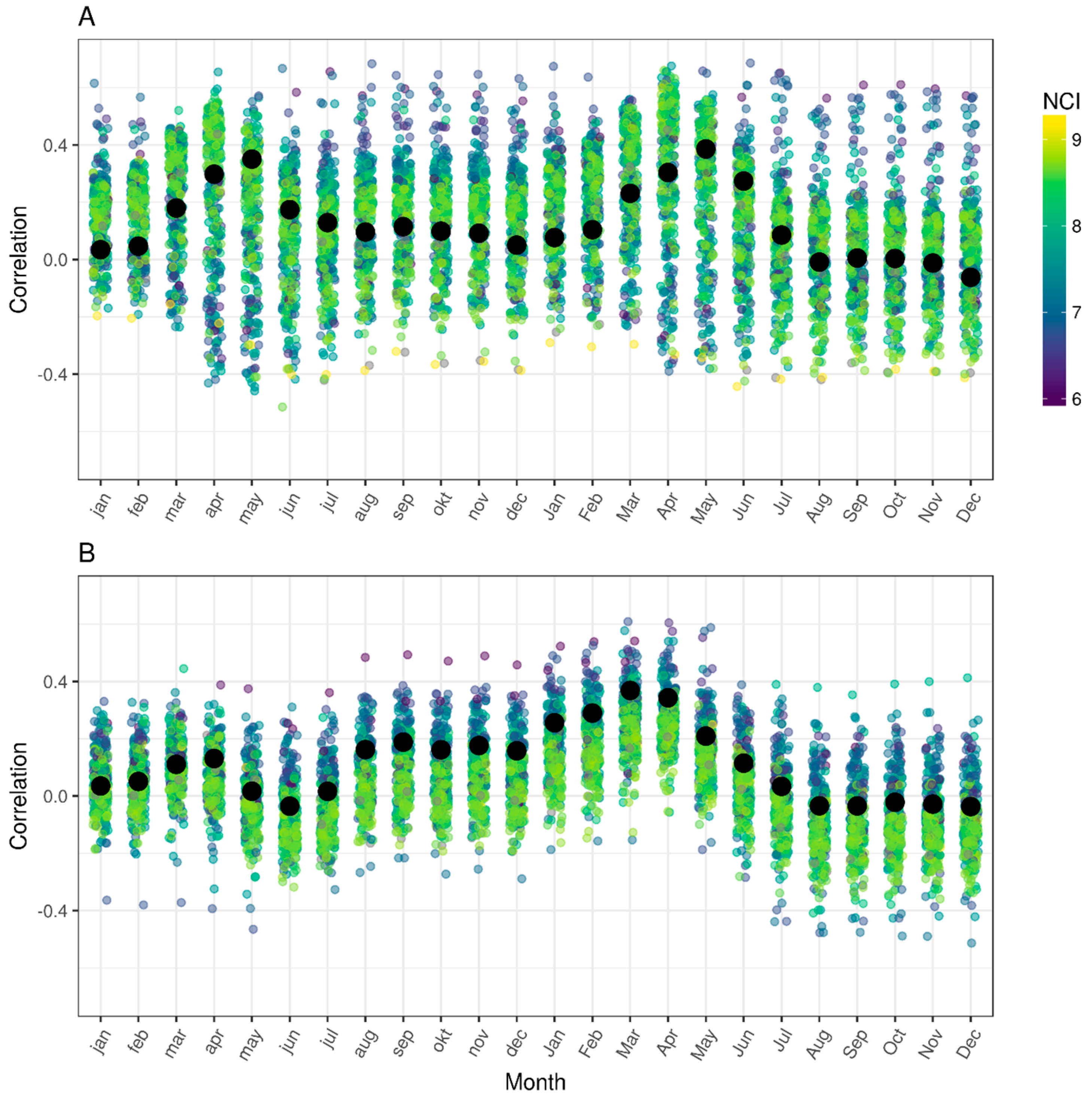
3.1. Jitterplots
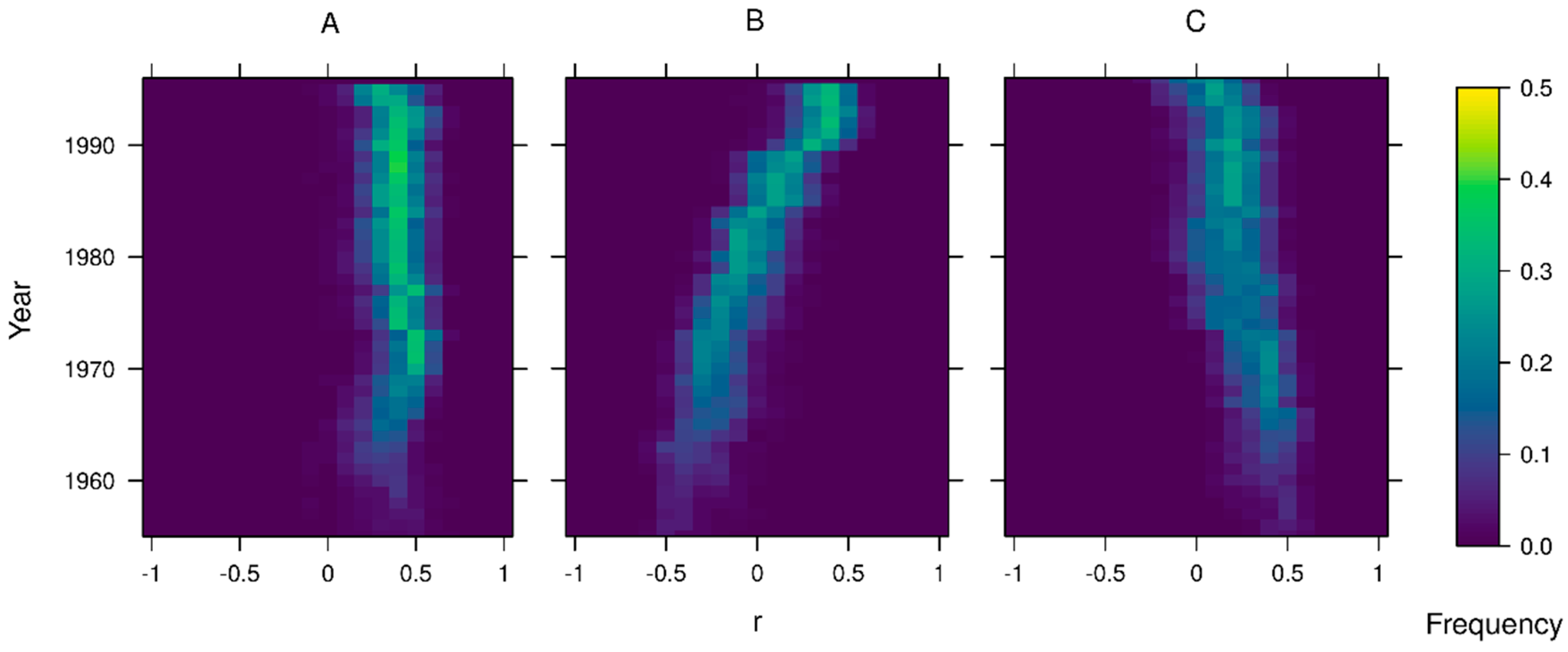
3.2. Individual Tree Moving Window Correlations
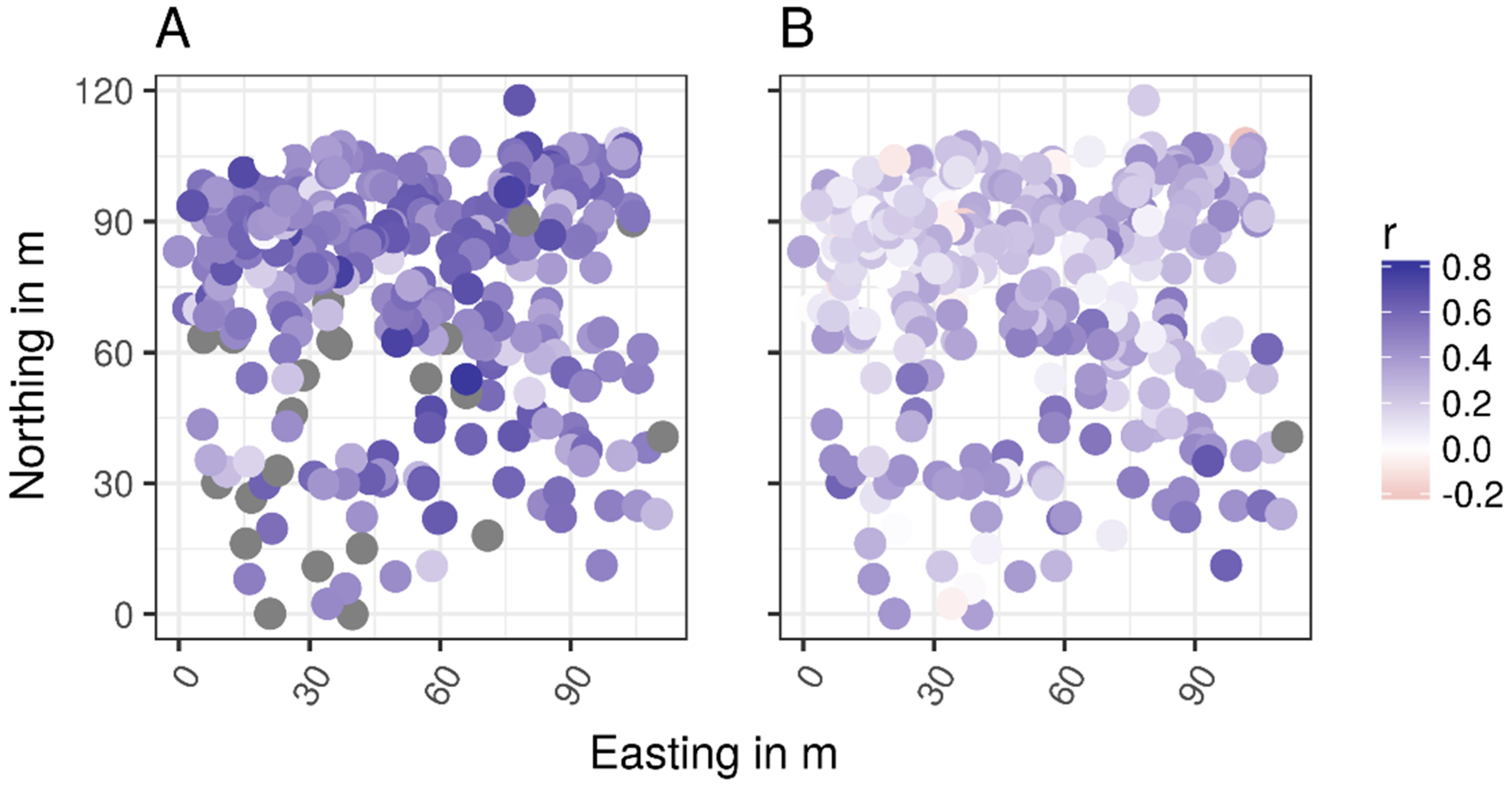
3.3. Spatial Distribution Maps
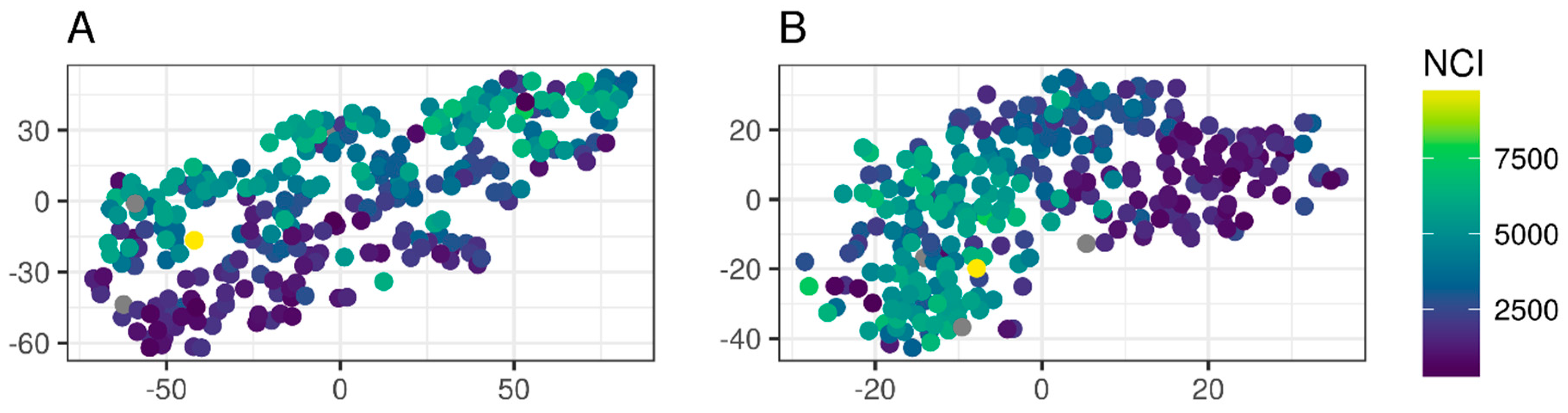
3.4. Similar Tree Ring Patterns and Climate Sensitivity
4. Discussion
4.1. Variances
4.2. Individual Metadata Effects on Climate Sensitivity
4.3. Potential Further Analyses
5. Conclusions
Supplementary Materials
Acknowledgments
Author Contributions
Conflicts of Interest
References
- Cook, E.R.; Kairiukstis, L.A. Methods of Dendrochronology: Applications in the Environmental Sciences; Springer Science & Business Media: Dordrecht, The Netherlands, 2013; ISBN 978-94-015-7879-0. [Google Scholar]
- Fritts, H.C. Tree Rings and Climate; The Blackburn Press: Caldwell, NJ, USA, 1976; ISBN 978-1-930665-39-2. [Google Scholar]
- Speer, J.H. Fundamentals of Tree-Ring Research; University of Arizona Press: Tucson, AZ, USA, 2010. [Google Scholar]
- Hurlbert, S.H. Pseudoreplication and the design of ecological field experiments. Ecol. Monogr. 1984, 54, 187–211. [Google Scholar] [CrossRef]
- Zuur, A.F. Mixed Effects Models and Extensions in Ecology with R; Statistics for Biology and Health; Springer: New York, NY, USA, 2009. [Google Scholar]
- Lloyd, A.H.; Sullivan, P.F.; Bunn, A.G. Integrating dendroecology with other disciplines improves understanding of upper and latitudinal treelines. In Dendroecology; Ecological Studies; Springer: Cham, Switzerland, 2017; pp. 135–157. [Google Scholar]
- Cook, E.R. A Time Series Analysis Appoach to Tree Ring Standardization. Ph.D. Thesis, University of Arizona, Tucson, AZ, USA, 1985. [Google Scholar]
- Kelly, D. The evolutionary ecology of mast seeding. Trends Ecol. Evol. 1994, 9, 465–470. [Google Scholar] [CrossRef]
- Martin-Benito, D.; Kint, V.; del Río, M.; Muys, B.; Cañellas, I. Growth responses of West-Mediterranean Pinus nigra to climate change are modulated by competition and productivity: Past trends and future perspectives. For. Ecol. Manag. 2011, 262, 1030–1040. [Google Scholar] [CrossRef]
- Sullivan, P.F.; Pattison, R.R.; Brownlee, A.H.; Cahoon, S.M.P.; Hollingsworth, T.N. Limited evidence of declining growth among moisture-limited black and white spruce in interior Alaska. Sci. Rep. 2017, 7, 15344. [Google Scholar] [CrossRef] [PubMed]
- Sherriff, R.L.; Miller, A.E.; Muth, K.; Schriver, M.; Batzel, R. Spruce growth responses to warming vary by ecoregion and ecosystem type near the forest-tundra boundary in south-west Alaska. J. Biogeogr. 2017, 44, 1457–1468. [Google Scholar] [CrossRef]
- Schweingruber, F.H.; Kairiukstis, L.; Shiyatov, S. Sample Selection. In Methods of Dendrochronology: Applications in the Environmental Sciences; Cook, E.R., Kairiukstis, L.A., Eds.; Springer Science & Business Media: Dordrecht, The Netherlands, 1990. [Google Scholar]
- Körner, C. Alpine Treelines: Functional Ecology of the Global High Elevation Tree Limits; Springer Science & Business Media: Basel, Switzerland; Heidelberg, Germany; New York, NY, USA; Dordrecht, The Netherlands; London, UK, 2012. [Google Scholar]
- Wigley, T.M.L.; Briffa, K.R.; Jones, P.D. On the average value of correlated time series, with applications in dendroclimatology and hydrometeorology. J. Clim. Appl. Meteorol. 1984, 23, 201–213. [Google Scholar] [CrossRef]
- Douglass, A. Climate Cycles and Tree-growth; Carnegie Institution of Washington: Washington, DC, USA, 1936. [Google Scholar]
- Bunn, A.G.; Jansma, E.; Korpela, M.; Westfall, R.D.; Baldwin, J. Using simulations and data to evaluate mean sensitivity (ζ) as a useful statistic in dendrochronology. Dendrochronologia 2013, 31, 250–254. [Google Scholar] [CrossRef]
- Buras, A. A comment on the expressed population signal. Dendrochronologia 2017, 44, 130–132. [Google Scholar] [CrossRef]
- Trugman, A.T.; Medvigy, D.; Anderegg, W.R.L.; Pacala, S.W. Differential declines in Alaskan boreal forest vitality related to climate and competition. Glob. Chang Biol. 2018. [Google Scholar] [CrossRef] [PubMed]
- Price, D.T.; Cooke, B.J.; Metsaranta, J.M.; Kurz, W.A. If forest dynamics in Canada’s west are driven mainly by competition, why did they change? Half-century evidence says: Climate change. Proc. Natl. Acad. Sci. USA 2015, 112, E4340. [Google Scholar] [CrossRef] [PubMed]
- Zhang, J.; Huang, S.; He, F. Half-century evidence from western Canada shows forest dynamics are primarily driven by competition followed by climate. Proc. Natl. Acad. Sci. USA 2015, 112, 4009–4014. [Google Scholar] [CrossRef] [PubMed]
- Wang, Y.; Pederson, N.; Ellison, A.M.; Buckley, H.L.; Case, B.S.; Liang, E.; Julio Camarero, J. Increased stem density and competition may diminish the positive effects of warming at alpine treeline. Ecology 2016, 97, 1668–1679. [Google Scholar] [CrossRef] [PubMed]
- Konter, O.; Krusic, P.J.; Trouet, V.; Esper, J. Meet Adonis, Europe’s oldest dendrochronologically dated tree. Dendrochronologia 2017, 42, 12. [Google Scholar] [CrossRef]
- Turney, C.S.M.; Palmer, J.; Maslin, M.A.; Hogg, A.; Fogwill, C.J.; Southon, J.; Fenwick, P.; Helle, G.; Wilmshurst, J.M.; McGlone, M.; et al. Global peak in atmospheric radiocarbon provides a potential definition for the onset of the anthropocene epoch in 1965. Sci. Rep. 2018, 8, 3293. [Google Scholar] [CrossRef] [PubMed]
- Carrer, M. Individualistic and time-varying tree-ring growth to climate sensitivity. PLoS ONE 2011, 6, e22813. [Google Scholar] [CrossRef] [PubMed]
- Gleason, K.E.; Bradford, J.B.; Bottero, A.; D’Amato, A.W.; Fraver, S.; Palik, B.J.; Battaglia, M.A.; Iverson, L.; Kenefic, L.; Kern, C.C. Competition amplifies drought stress in forests across broad climatic and compositional gradients. Ecosphere 2017, 8. [Google Scholar] [CrossRef]
- Choler, P.; Michalet, R.; Callaway, R.M. Facilitation and competition on gradients in alpine plant communities. Ecology 2001, 82, 3295–3308. [Google Scholar] [CrossRef]
- Callaway, R.M.; Walker, L.R. Competition and facilitation: A synthetic approach to interactions in plant communities. Ecology 1997, 78, 1958–1965. [Google Scholar] [CrossRef]
- Rohner, B.; Waldner, P.; Lischke, H.; Ferretti, M.; Thürig, E. Predicting individual-tree growth of central European tree species as a function of site, stand, management, nutrient, and climate effects. Eur. J. For. Res. 2017, 1–16. [Google Scholar] [CrossRef]
- Konter, O.; Büntgen, U.; Carrer, M.; Timonen, M.; Esper, J. Climate signal age effects in boreal tree-rings: Lessons to be learned for paleoclimatic reconstructions. Quat. Sci. Rev. 2016, 142, 164–172. [Google Scholar] [CrossRef]
- Galván, J.D.; Camarero, J.J.; Gutiérrez, E. Seeing the trees for the forest: Drivers of individual growth responses to climate in Pinus uncinata mountain forests. J. Ecol. 2014, 102, 1244–1257. [Google Scholar] [CrossRef]
- Buras, A.; van der Maaten-Theunissen, M.; van der Maaten, E.; Ahlgrimm, S.; Hermann, P.; Simard, S.; Heinrich, I.; Helle, G.; Unterseher, M.; et al. Tuning the voices of a choir: Detecting ecological gradients in time-series populations. PLoS ONE 2016, 11, e0158346. [Google Scholar] [CrossRef] [PubMed]
- Ibáñez, I.; Zak, D.R.; Burton, A.J.; Pregitzer, K.S. Anthropogenic nitrogen deposition ameliorates the decline in tree growth caused by a drier climate. Ecology 2018, 99, 411–420. [Google Scholar] [CrossRef] [PubMed]
- Driscoll, W.W.; Wiles, G.C.; D’Arrigo, R.D.; Wilmking, M. Divergent tree growth response to recent climatic warming, Lake Clark National Park and Preserve, Alaska. Geophys. Res. Lett. 2005, 32, L20703. [Google Scholar] [CrossRef]
- Zhang, Y.; Wilmking, M. Divergent growth responses and increasing temperature limitation of Qinghai spruce growth along an elevation gradient at the northeast Tibet Plateau. For. Ecol. Manag. 2010, 260, 1076–1082. [Google Scholar] [CrossRef]
- Wilmking, M.; D’Arrigo, R.; Jacoby, G.C.; Juday, G.P. Increased temperature sensitivity and divergent growth trends in circumpolar boreal forests. Geophys. Res. Lett. 2005, 32, L15715. [Google Scholar] [CrossRef]
- Ponocná, T.; Chuman, T.; Rydval, M.; Urban, G.; Migaɬa, K.; Treml, V. Deviations of treeline Norway spruce radial growth from summer temperatures in East-Central Europe. Agric. For. Meteorol. 2018, 253–254, 62–70. [Google Scholar] [CrossRef]
- D’Arrigo, R.; Wilson, R.; Liepert, B.; Cherubini, P. On the ‘Divergence Problem’ in Northern Forests: A review of the tree-ring evidence and possible causes. Glob. Planet. Chang. 2008, 60, 289–305. [Google Scholar] [CrossRef]
- Wilmking, M.; Juday, G.P. Longitudinal variation of radial growth at Alaska’s northern treeline—recent changes and possible scenarios for the 21st century. Glob. Planet. Chang. 2005, 47, 282–300. [Google Scholar] [CrossRef]
- Wilmking, M.; Buras, A.; Eusemann, P.; Schnittler, M.; Trouillier, M.; Würth, D.; Lange, J.; van der Maaten-Theunissen, M.; Juday, G.P. High frequency growth variability of White spruce clones does not differ from non-clonal trees at Alaskan treelines. Dendrochronologia 2017, 44, 187–192. [Google Scholar] [CrossRef]
- Housset, J.M.; Nadeau, S.; Isabel, N.; Depardieu, C.; Duchesne, I.; Lenz, P.; Girardin, M.P. Tree rings provide a new class of phenotypes for genetic associations that foster insights into adaptation of conifers to climate change. New Phytol. 2018. [Google Scholar] [CrossRef] [PubMed]
- King, G.M.; Gugerli, F.; Fonti, P.; Frank, D.C. Tree growth response along an elevational gradient: Climate or genetics? Oecologia 2013, 173, 1587–1600. [Google Scholar] [CrossRef] [PubMed]
- Gärtner, H.; Nievergelt, D. The core-microtome: A new tool for surface preparation on cores and time series analysis of varying cell parameters. Dendrochronologia 2010, 28, 85–92. [Google Scholar] [CrossRef]
- Cybis Elektronik & Data AB. In CooRecorder; Saltsjöbaden, Sweden. Available online: http://www.cybis.se/indexe.htm (accessed on 19 April 2018).
- Canham, C.D.; LePage, P.T.; Coates, K.D. A neighborhood analysis of canopy tree competition: Effects of shading versus crowding. Can. J. For. Res. 2004, 34, 778–787. [Google Scholar] [CrossRef]
- SNAP Scenarios Network for Alaska and Arctic Planning 2016; University of Alaska, Fairbanks, USA. Available online: http://ckan.snap.uaf.edu/dataset (accessed on 19 April 2018).
- Vicente-Serrano, S.M.; Beguería, S.; López-Moreno, J.I. A multiscalar drought index sensitive to global warming: The standardized precipitation evapotranspiration index. J. Clim. 2009, 23, 1696–1718. [Google Scholar] [CrossRef]
- Beguería, S.; Vicente-Serrano, S.M. SPEI: Calculation of the Standardised Precipitation-Evapotranspiration Index; R Package Version 1.6. 2013. Available online: https://CRAN.R-project.org/package=SPEI (accessed on 19 April 2018).
- Bunn, A.G. A dendrochronology program library in R (dplR). Dendrochronologia 2008, 26, 115–124. [Google Scholar] [CrossRef]
- R Core Team. R: A Language and Environment for Statistical Computing; R Foundation for Statistical Computing: Vienna, Austria, 2015. [Google Scholar]
- Zang, C.; Biondi, F. treeclim: An R package for the numerical calibration of proxy-climate relationships. Ecography 2015, 38, 431–436. [Google Scholar] [CrossRef]
- Wickham, H. ggplot2: Elegant Graphics for Data Analysis; Springer: New York, NY, USA, 2009. [Google Scholar]
- Wilmking, M.; Scharnweber, T.; van der Maaten-Theunissen, M.; van der Maaten, E. Reconciling the community with a concept—The uniformitarian principle in the dendro-sciences. Dendrochronologia 2017, 44, 211–214. [Google Scholar] [CrossRef]
- Lloyd, S. Least squares quantization in PCM. IEEE Trans. Inf. Theory 1982, 28, 129–137. [Google Scholar] [CrossRef]
- Van der Maaten, L.; Hinton, G. Visualizing Data using t-SNE. J. Mach. Learn. Res. 2008, 9, 2579–2605. [Google Scholar]
- Krijthe, J.H. Rtsne: T-Distributed Stochastic Neighbor Embedding Using Barnes-Hut Implementation. 2015. Available online: https://github.com/jkrijthe/Rtsne (accessed on 19 April 2018).
- Mencuccini, M.; Hölttä, T.; Petit, G.; Magnani, F. Sanio’s laws revisited. Size-dependent changes in the xylem architecture of trees. Ecol. Lett. 2007, 10, 1084–1093. [Google Scholar] [CrossRef] [PubMed]
- Carrer, M.; Urbinati, C. Age-dependent tree-ring growth responses to climate in Larix Decidua and Pinus Cembra. Ecology 2004, 85, 730–740. [Google Scholar] [CrossRef]
- King, D.A. The Adaptive Significance of Tree Height. Am. Nat. 1990, 135, 809–828. [Google Scholar] [CrossRef]
- Koch, G.W.; Sillett, S.C.; Jennings, G.M.; Davis, S.D. The limits to tree height. Nature 2004, 428, 851–854. [Google Scholar] [CrossRef] [PubMed]
- Weiner, J. Asymmetric competition in plant populations. Trends Ecol. Evol. 1990, 5, 360–364. [Google Scholar] [CrossRef]
- Pretzsch, H.; Biber, P. Size-symmetric versus size-asymmetric competition and growth partitioning among trees in forest stands along an ecological gradient in central Europe. Can. J. For. Res. 2010, 40, 370–384. [Google Scholar] [CrossRef]
- Linares, J.-C.; Delgado-Huertas, A.; Camarero, J.J.; Merino, J.; Carreira, J.A. Competition and drought limit the response of water-use efficiency to rising atmospheric carbon dioxide in the Mediterranean fir Abies pinsapo. Oecologia 2009, 161, 611–624. [Google Scholar] [CrossRef] [PubMed]
- Sanio, K. Uber die Grosse der Holzzellen bei der Gemeinen Kiefer (Pinus silvestris); Leipzig publisher: Leipzig, Saxony, Germany, 1872; pp. 401–420. [Google Scholar]
- Ryan, M.G.; Yoder, B.J. Hydraulic limits to tree height and tree growth. BioScience 1997, 47, 235–242. [Google Scholar] [CrossRef]
- Ryan Michael, G.; Phillips, N.; Bond Barbara, J. The hydraulic limitation hypothesis revisited. Plant Cell Environ. 2006, 29, 367–381. [Google Scholar] [CrossRef]
- Alam, S.A.; Huang, J.-G.; Stadt, K.J.; Comeau, P.G.; Dawson, A.; Gea-Izquierdo, G.; Aakala, T.; Hölttä, T.; Vesala, T.; Mäkelä, A.; Berninger, F. Effects of competition, drought stress and photosynthetic productivity on the radial growth of White Spruce in Western Canada. Front. Plant Sci. 2017, 8. [Google Scholar] [CrossRef] [PubMed]
- Bates, D.; Mächler, M.; Bolker, B.; Walker, S. Fitting linear mixed-effects models using lme4. arXiv 2014, 67, 1. [Google Scholar] [CrossRef]
- Vaganov, E.A.; Hughes, M.K.; Shashkin, A.V. Growth Dynamics of Conifer Tree Rings: Images of Past and Future Environments; Springer Science & Business Media: Dordrecht, The Netherlands, 2006. [Google Scholar]
- Vaganov, E.A.; Anchukaitis, K.J.; Evans, M.N. How Well Understood Are the Processes that Create Dendroclimatic Records? A Mechanistic Model of the Climatic Control on Conifer Tree-Ring Growth Dynamics. In Dendroclimatology; Developments in Paleoenvironmental Research; Springer: Dordrecht, The Netherlands, 2011; pp. 37–75. [Google Scholar]
- Pretzsch, H.; Biber, P.; Ďurský, J.; von Gadow, K.; Hasenauer, H.; Kändler, G.; Kenk, G.; Kublin, E.; Nagel, J.; Pukkala, T.; et al. Recommendations for standardized documentation and further development of forest growth simulators. Forstw. Cbl. 2002, 121, 138–151. [Google Scholar] [CrossRef]
- Grimm, V.; Railsback, S.F. Individual-Based Modeling and Ecology; Princeton University Press: Princeton, NJ, USA, 2013. [Google Scholar]


© 2018 by the authors. Licensee MDPI, Basel, Switzerland. This article is an open access article distributed under the terms and conditions of the Creative Commons Attribution (CC BY) license (http://creativecommons.org/licenses/by/4.0/).
Share and Cite
Trouillier, M.; Van der Maaten-Theunissen, M.; Harvey, J.E.; Würth, D.; Schnittler, M.; Wilmking, M. Visualizing Individual Tree Differences in Tree-Ring Studies. Forests 2018, 9, 216. https://doi.org/10.3390/f9040216
Trouillier M, Van der Maaten-Theunissen M, Harvey JE, Würth D, Schnittler M, Wilmking M. Visualizing Individual Tree Differences in Tree-Ring Studies. Forests. 2018; 9(4):216. https://doi.org/10.3390/f9040216
Chicago/Turabian StyleTrouillier, Mario, Marieke Van der Maaten-Theunissen, Jill E. Harvey, David Würth, Martin Schnittler, and Martin Wilmking. 2018. "Visualizing Individual Tree Differences in Tree-Ring Studies" Forests 9, no. 4: 216. https://doi.org/10.3390/f9040216