An Inventory-Based Regeneration Biomass Model to Initialize Landscape Scale Simulation Scenarios


Chair of Forest Growth and Yield Science, Technical University of Munich, Hans-Carl-von-Carlowitz-Platz 2, 85354 Freising, Germany
*
Author to whom correspondence should be addressed.
Forests 2018, 9(4), 212; https://doi.org/10.3390/f9040212
Submission received: 18 March 2018
/
Revised: 5 April 2018
/
Accepted: 12 April 2018
/
Published: 17 April 2018
(This article belongs to the Special Issue Simulation Modeling of Forest Ecosystems)
Abstract
:Dynamic landscape simulation of the forest requires an initial regeneration stock specific to the characteristics of each simulated stand. Forest inventories, however, are sparse with regard to regeneration. Moreover, statistical regeneration models are rare. We introduce an inventory-based statistical model type that (1) quantifies regeneration biomass as a fundamental regeneration attribute and (2) uses the overstory’s quadratic mean diameter (Dq) together with several other structure attributes and the Site Index as predictors. We form two such models from plots dominated by European beech (Fagus sylvatica L.), one from national forest inventory data and the other from spatially denser federal state forest inventory data. We evaluate the first one for capturing the predictors specific to the larger scale level and the latter one to infer the degree of landscape discretization above which the model bias becomes critical due to yet unquantified determinants of regeneration. The most relevant predictors were Dq, stand density, and maximum height (significance level p < 0.0001). If plot data sets for evaluation differed by the forest management unit in addition to the average diameter, the bias range among them increased from 0.1-fold of predicted biomass to 0.3-fold.
1. Introduction
The dynamic simulation of forest growth and structure development is an essential prerequisite to future scenarios that consider ecosystem service provision on a landscape level [1]. In order to start from a realistic representation of the forest in its current state, scenarios require data of the stand structures present within the landscape considered. Sample plots are the primary inventory unit in modern grid-based forest inventories. They provide detailed structure data for modelling and are widely available. However, they have a distance of up to several kilometers from each other.
A proven method that approximately represents the forest stand structures within a landscape groups all available inventory plots into strata [2,3]. Such a stratification classifies plots by stand structure attributes, as well as site quality. Typically, it then uses the data of all inventory plots from a given stratum to construct a virtual forest stand. That virtual stand serves to simulate the stratum’s development within a representative subunit [4] (p. 502 ff.). The stratification method yields a good representation of the overstory per stratum, here defined as all trees with a minimum diameter at breast height (DBH) of 7 cm. However, this is much less the case for the understory: it consists of the young trees with a DBH of less than 7 cm that form the basis of the next stand generation. Typical inventories [5,6] sample regeneration in very small sub-areas within an inventory plot, while, conversely, the stand intrinsic variability of regeneration is large [7]. Thus, within a stratum considered, there might often not be enough inventory plots to provide a statistically stable estimation of its regeneration stock. Moreover, remote sensing will likely support terrestrial inventories in the near future and might even substitute them in some areas or cover regions where forest inventories are completely missing so far [8,9,10]. Except under very sparse main stands, regeneration trees will almost be undetectable by remote sensors. Therefore, simulation scenarios on the forest landscape level will benefit from a statistical method that, based on overstory structure and site [11,12,13], contributes a quantitative estimation of regeneration stock to each stratum. That estimation is an essential starting condition for dynamically simulating the ingrowth of regeneration trees into the main stand. Ingrowth, in turn, is the crucial process for the change of forest stand generations and, thus, a key process for adaptation to climate change.
The density of regeneration trees within a stand typically varies on a spatial scale of only a few square meters [7,14,15]. A notable part of that variation will be due to stochastic effects, such as felling damages and small-scale game browsing within small understory sectors. Statistical models of regeneration, thus, will not precisely predict the understory stock within such a small-scale stand sector, even if they would account for any relevant structure attribute of the sector’s local overstory. Still, such a model might infer the probability distribution of the stand sector’s regeneration stock from the sector’s local overstory structure. A realistic case of model application, thus, is to derive a representative collection of such sector-related regeneration stock distributions within a whole stratum from a known set of structure types within the stratum’s overstory. That distribution set, through random sampling from each local distribution, could then provide a realistic initial pattern of regeneration within a virtual stand.
Scenarios of forest growth and structure development are typically based on dynamic simulation models. To represent growth within the regeneration layer, or even within the overstory, such models often discretize a given virtual stand into a regular pattern of quadratic tiles with an edge length of 2.5 to 20 m. That way, they take into account the variability of regeneration stock at the horizontal resolution of small-scale effects. Prominent examples are the regeneration module of SILVA [16] and modern patch models [17,18].
National forest inventory (NFI) data are ideal to calibrate a statistical model for regeneration stock. Such a model would cover a wide range of overstory structures and site quality. It would yield the specific distribution of plot-wise regeneration stock at a given overstory structure and given site properties, obtained from a large data set. A straightforward approach for initializing tiles within a stratum-based virtual stand might assume that such a predictor-related distribution is applicable to represent the distribution within any plot-sized stand subsector of corresponding predictor values. Based on a sample of stratum-related overstory attributes, it would first evaluate the overstory surrounding the tile of interest. The result is then related to a specific distribution of regeneration stock. Conveniently, subplots where regeneration is sampled and model tiles are of a similar size. Thus, the algorithm would take a random sample of the tile’s regeneration stock directly from the tile-related distribution.
However, any structure-related distribution of regeneration stock from an NFI-based model results from a convolution of many distributions: due to the model’s comprehensive data basis, each of them is specific to one of numerous distinct sub regions. On a large national scale level, due to a landscape-related browsing intensity and other regional factors [19], strata of a similar structure and similar site properties might notably differ in their relation between overstory structure and regeneration stock. Model design may counteract such variation by striving for predictors that correlate as closely as possible with biological processes and silvicultural practices. Still, the model’s realism will strongly depend on the level of stratum differentiation and discretization that the model user intends.
The study at hand conceptualizes an inventory-based model type that aims to predict the regeneration stock distribution per stratum based on the stratum-intrinsic overstory pattern and the stratum’s site properties. In order to obtain the distribution per stratum, the model estimates the distribution of regeneration stock per plot-sized sub-area of the stratum’s virtual stand and samples one value per sub-area related distribution. Within that scope, the study follows two fundamental objectives. The first one is to identify important predictors of regeneration biomass within the large spatial scope of the German state territory (36 million ha with 11 million ha of forest).
More detailed stratification criteria will result in more appropriate management strategies per stratum during simulation. However, using highly detailed criteria is also related to high level of forest landscape discretization. More profound stratification, thus, might lead to smaller strata that differ in their average regeneration stock due to stochastic variation among them. Hence, such stratification might impair the precision of a statistical regeneration model. The second fundamental objective, therefore, is to estimate the degree of stratum differentiation, beyond which the model produces a critical bias of the per-stratum average. To meet both fundamental objectives of the study, we design two closely related model versions: one uses data from the German National Forest Inventory (referred to as NFI in the following). That inventory covers the total German forest area. However, due to its spatial resolution (4 km × 4 km), it is not ideal for analyzing the model performance on the spatial level of landscape-related simulation scenarios (about 50,000 ha of forest). Therefore, the study uses a second model version that is based on the exceptionally dense Bavarian State Forest Inventory (BSFI, 200 m × 200 m). That inventory covers a state forest area of almost 1 million ha. In order to determine the limit of spatial resolution that our modelling approach currently has, we evaluated the bias of the BSFI-based model as dependent on the differentiation of strata formed from BSFI plots on two different discretization levels.
Both models use the aboveground regeneration biomass within each plot as a dependent variable that is closely linked to net primary production [20]. As the height of regeneration on the plot scale may be highly heterogeneous [11], regeneration biomass represents resource supply more directly than the total number of regeneration trees per plot.
At the current state of model development, our study focuses on plots dominated by European beech (Fagus sylvatica L.) within the overstory. European beech is by far the most important broadleaved species in Central Europe. As it is shade tolerant, it occurs along a broad range of stand structures and sites. Moreover, it primarily regenerates through natural seed dispersion.
2. Materials and Methods
2.1. Data
On the national scale level, the study at hand used the German National Forest Inventory (NFI, 4 km grid) that covers the whole forest area of Germany. The version of these data was the third and most recent survey conducted in 2011 and 2012 [6] with reference date 1 October 2012 [21]. For evaluating the bias of the BSFI-based model as related to the resolution of strata, the study applied plot data from the Bavarian State Forest Inventory that covers the forest area managed by the Federal State of Bavaria (BSFI in the further text, 200 m grid). The BSFI surveys 41 forest management units with an average size of about 20,000 ha, each at a repeat cycle of 10 years. Per each forest management unit, it applies individual due dates.
2.1.1. German National Forest Inventory (NFI)
The German National Forest Inventory (description mostly taken from [6]) is based on a regular 4 km × 4 km quadrangle grid that covers the entire national forest area (~11,400,000 ha, 59,858 plots). It is denser inside some federal states where it has a 2.83 km × 2.83 km or 2 km × 2 km grid. Each grid point represents a north-to-south oriented square with an edge length of 150 m. At the corners of each square, there is exactly one inventory plot, so that the square represents an inventory cluster. On all plots, the NFI measures the overstory (trees of DBH ≥ 7) around each plot center as an angle count sample with a standard basal area factor (BAF) of 4. In addition, it takes the DBH of each sampled tree. Based on the BAF and measured DBH, overstory stem densities per ha are calculated. Within most plots, height measurements are collected on a subset. In continuous cover forests, however, the heights of all sampled trees are measured.
Regeneration trees (DBH < 7 cm) are surveyed within two concentric circles that are situated 5 m north of the plot center. To that end, small saplings with a height of at least 0.2 m and less than 0.5 m are counted on the inner circle of a 1 m radius. Understory trees with a height of at least 0.5 m are counted on the outer circle that has a 2 m radius. Within that circle, the counted trees are attributed to different size classes. The first class comprises trees with a height of less than 1.3 m (and at least 0.5 m). Higher trees are attributed to the DBH classes 0 to 5 cm, 5 to 6 cm, and 6 to 7 cm (upper limits excluded). The radius of the inner circle is extended to 2 m if it would comprise less than four trees within the default radius of 1 m. The NFI registers the browsing of regeneration by an annotation per tree size class. A total of 46% of all plots with a beech-dominated overstory and regeneration had been marked as being browsed by ungulates in at least one regeneration size class.
Within this regeneration survey, the NFI computes regeneration biomass per tree size class from height if the tree considered is less than 1.3 m high and, furthermore, as based on diameter if the tree is higher [22,23]. The height-based part of the biomass calculation, to that end, uses one standard height per class, one of 0.35 m (for height class 0.2 to 0.5 m) and one of 0.9 m (>0.5 m to 1.3 m). It applies one generalist biomass to height relation for either coniferous or broadleaved species. On the contrary, the diameter-based biomass estimation interpolates between the height-based biomass at a height of 1.3 m and a species-specific biomass value at a DBH of 10 cm calculated with a modified Marklund model [24]. For model calibration and evaluation, we selected a subset of 7823 inventory plots with a basal area (BA) share of beech that was more than 55% within the overstory. That data set will be denoted as “NFI data” in the following (Table 1).
The total BA shares within that set were 84% for beech and 93% for deciduous species in general. We classified 48% of all selected plots as beech monoculture (BA share > 90%). Within the set of beech-dominated plots, the share of regeneration biomass was 74% for beech and 92% for deciduous. Furthermore, 30% of the plots had a regeneration biomass of zero.
2.1.2. Bavarian State Forest Inventory (BSFI)
In contrast to the NFI, which has mainly monitoring purposes, the BSFI is designed to support forest management planning on the level of forest management units (20,000 ha). Therefore, it uses a much higher spatial sampling density on a square grid of a 200 m grid width on average. Each inventory unit is a circular plot with an area of 400 to 500 m2 that encloses several smaller concentric inventory circles. Only trees above a certain threshold DBH (typically 30 cm) are recorded on the whole plot area. Trees with a DBH < 30 cm and ≥ 11 cm are measured within an 80 to 125 m2 circle. The smallest class of trees with a DBH < 11 cm, including regeneration trees, is surveyed on a 25 m2 circle [25]. The minimum height of regeneration trees to be sampled in the BSFI is 0.2 m, the same as in the NFI. Trees up to a height of 1.3 m are recorded at a higher-class width, i.e., 0.1 m. Trees of a DBH > 0 and < 7 cm are recorded per DBH levels 1.5, 2.5, 3.5, 4.5, 5.5, and 6.5 cm. The beech-dominated BSFI data set used for model calibration and evaluation was selected by the same criteria as the NFI data. That set of plots with beech-dominated overstory will be named “BSFI data” in the following (Table 2).
The study comprised 11,954 plots from 26 spatially independent inventories over the federal state of Bavaria that had been taken within different years for the period from 2003 to 2012. The basal area shares within the BSFI data were 84% for beech and 91% for deciduous. A total of 41% of all plots were beech monoculture. In order to maintain consistency between NFI and BSFI data, we calculated the regeneration biomass per BSFI plot with the biomass algorithm of the NFI. The share of regeneration biomass then was 76% for beech and 89% for deciduous. Within the BSFI data, 29% of the plots had a regeneration biomass of zero. BSFI plot data, in difference to NFI data, have two topological keys: one that refers to the enclosing forest stand and one that is unique to the enclosing forest management unit. A total of 6073 of the 11,954 plots were spared from model calibration to form strata of a sufficient size for evaluation. Thus, half of all, i.e., 5881 plots remained to parameterize the BSFI-based model.
2.2. Data Preparation
The BSFI surveys regeneration trees within a larger collective of DBH < 11 cm. Again, to keep regeneration tree data from NFI and BSFI consistent with each other, we confined regeneration trees from both inventories to the group with a DBH < 7 cm.
Based on an ecophysiological perception of the regeneration process [26,27], we derived a set of overstory characteristics from the inventory plot data that likely determine regeneration biomass. These properties represent above and belowground competition, growth potential, and stand maturity. Both the NFI- and the BSFI-based model use the same set of predictors. In order to parameterize each model, we computed one independent set of plot-related predictor values per each inventory. For quantifying the overstory stand density, we used the Stand Density Index (SDI) [28] which enables a comparison of stand densities at very different development stages. This structure indicator has been shown to be an effective predictor of regeneration in previous work on experimental plots [29]. It is defined through Equation (1):
where N is the number of trees per ha and Dq is the quadratic mean diameter in cm. The SDI may be considered to represent the spatial concentration of tree biomass [4] (p. 399 ff.). Thus, it is a comprehensive indicator of the degree of competition for above- and belowground resources.
While the SDI expresses the current stand density at the time of measurement, we also required a variable that indicates whether a stand has been kept at higher or lower densities in the long run, because a low density could also result from heavy thinning in a previously dense stand. Therefore, we developed a method for quantifying whether an overstory tree is slender or stout, or has a normal height for its DBH. As a benchmark for normal heights at a given DBH, we fitted an allometric height-diameter model to overstory tree height and diameter (equation with parameters in Appendix A). Based on the residuals of that model, we estimated a DBH-related probability distribution to standardize the deviation between actual height and normal, i.e., expected height. That distribution enables us to introduce the Height Diameter Characteristic, HD. HD is defined as the probability (P) that any tree of the same diameter might be equally or less high (Equation (2)):
where h is height as a random variable, d is DBH as a predictor, and h0 and d0 are tree height and DBH as measured, respectively. Thus, HD can obtain any value between 0 and 1. For a tree of any diameter, HD = 0.5 indicates an average, i.e., normal height to diameter ratio. HD > 0.5 marks an above average tall tree and HD < 0.5 a stout one. That characteristic, hence, aims to indicate the extent to which a tree had been inhibited in diameter growth through neighbor competition in the past.
The Species Profile Index SPI [4] (p. 281 ff.) is a proxy for a forest stand’s richness in species and vertical structure simultaneously. High values indicate structurally rich stands and values of 0 indicate homogenous monospecific stands (Equation (3)):
where S is the number of species, Z is the number of height layers, and p is the relative frequency of species i in stand height layer j (exclusively species with pij > 0 considered). The Species Profile Index in its standard form is based on three stand height layers whose upper borders are Hmax × 1, Hmax × 0.8, and Hmax × 0.5, where Hmax is the maximum tree height in the stand of interest. SPI, thus, might indicate whether biomass is concentrated into exactly one tree class or shared among several ones within the stand being considered.
For quantifying the NFI and BSFI plots’ growth potential, we used a Site Index (SI), defined as the site dependent predominant tree height at age 100. It was computed by the site-productivity algorithm as implemented in the forest growth model SILVA [16]. That computation was based on the spatial position of the inventory plots and the German map of forest ecological regions [30]. Moreover, we included the Quadratic Mean Diameter (Dq) as a predictor that indicates the developmental state of the stand with respect to tree maturity for harvest. Stands with high Dq are in a phase where regeneration is promoted through felling. German forestry is marked by a large variety of treatment. Within one third of the forest, area transformation to uneven-aged stands and the maintenance of such stands is common. As an indicator of the stand’s development stage, thus, we used the maximum height per plot (Hmax) that is not limited to even-aged stands. Comparing both inventories by mean and range of corresponding native and derived variables, it can be seen that both are similar (Table 1 and Table 2).
2.3. Models
Both models, the NFI- and the BSFI-based version, have the same structure. With the key objective to estimate the local probability distribution of regeneration biomass within an inventory plot, each model comprised a deterministic part as well as a stochastic one. The deterministic module aims to predict the distribution’s expectancy value. As a complement, the stochastic part serves to estimate the variation around that predicted average. At the current stage of development, we aimed to restrict the presumptions for the deterministic module to a minimum. Accordingly, to predict regeneration biomass per ha B, we used a generalized additive mixed model (GAMM) for both the NFI-based model (Equation (4a)) and the BSFI-based one (Equation (4b)):
The fixed effects in this model are the Stand Density Index (SDI), the Species Profile Index (SPI), the Height Diameter Characteristic (HD), the stand maturity indicator (Hmax), the Site Index (SI), and the quadratic diameter (Dq). Except for Dq, all fixed effects in the model are linear (i.e., they are multiplied by one of the regression parameters β1, …, β5). In contrast, the effect of Dq is modeled with a nonlinear spline-based smoother [31], which is indicated by the symbol s(Dq). It accounts for a hypothesized nonlinear relation between Dq and regeneration stock due to a likely minimum of light transmission between the phase of adolescence and intense harvest.
In the model’s NFI-based version, the indices j and i associate any plot j to the corresponding four-plot cluster i. The BSFI-based version uses a further index k to represent the embedding of any plot k into the associated forest stand j and the enclosing forest management unit i. Variable r represents the deterministic part’s residuals, which deserve special attention. Due to the clustered data structure, r contains random effects on different levels. Within the NFI-based model, it comprises one single group effect that is due to the organization of plots within the inventory clusters (Equation (5)):
where bi is a cluster specific random effect and εij represents i.i.d. errors. The BSFI-based model comprises two group effects (Equation (6)):
where bi is the random effect related to the forest management unit and bij is the stand-related one. εijk represents the i.i.d. errors.
For fitting each model’s deterministic part (Equations (4a) resp. (4b)), we took into account that its absolute residuals (r in Equation (4)) might become larger as regeneration biomass (B) increases. In order to compensate for such heteroscedasticity, we applied a standard method [32] (p. 188).
Therefore, the deterministic part of the model (Equations (4a) resp. (4b)) was first calibrated to unweighted data to obtain the corresponding set of absolute residuals, i.e., the values of r. Then, a specific variance function (Equation (7)) was fitted to the squared residuals:
where r is the absolute residual, is the predicted biomass, and u and v are parameters to be estimated. Finally, the deterministic model part was fitted again with each observation weighted by the inverse of the residual variance as estimated through Equation (7). For fitting the deterministic part, we used the statistical software R [33] and the function gamm4 from package gamm4 [34]. The distribution assumption implied by the fitting procedure for Equation (4a) is bi ~ N(0, σ12) and εij ~ N(0, σ22). For fitting Equation (4b), we correspondingly assumed bi ~ N(0, σ32), bij ~ N(0, σ42), and εijk ~ N(0, σ52). In order to facilitate the reproduction and application of the deterministic model part, we complemented both Equations (4a) and (4b) with an approximation that refrained from the smoothing spline s(Dq). To that end, we replaced s(Dq) with a small set of polynomials. Therefore, we predicted regeneration biomass based on the observed Dq values and the mean of each remainder predictor. Then, we fit one polynomial to the data of predicted biomass over Dq within each of several Dq intervals.
The stochastic model part again uses an identical set of equations within the NFI- and the BSFI-based model. It aims to represent the typical spread of regeneration biomass values around an average value as predicted by Equations (4a) resp. (4b). Therefore, it describes the distribution of the deterministic part’s residuals. As these residuals turned out to be heteroscedastic, they were standardized through division by the corresponding predicted mean biomass to obtain relative residuals. For approximating the variability among such relative residuals, the stochastic model part applies the gamma probability density function that is a flexible function confined to positive values. It uses one parameter for shape and one for steepness (rate), as given by Equation (8):
for R > 0, where R is the randomly distributed relative residual. Both α (shape) and β (rate) are parameters (>0). Г denotes the Gamma function. To obtain parameter values for Equation (8) and to account for remaining heteroscedasticity, we estimated the function’s characteristics from the biomass predicted by the deterministic part. Therefore, the stochastic part uses linear trends of the distribution’s parameters shape α and rate β over predicted biomass (Equations (9a) and (9b)):
where is a biomass value predicted by Equations (4a) resp. (4b); u1, u2, v1, and v2 are regression parameters; and index l stands for an observation. Both ε1 ~ N(0, σ62) and ε2 ~ N(0, σ72) are the i.i.d. errors. In order to describe both trends, we divided the range of predicted biomass values into 40 intervals, each representing a quantile width of 2.5%. Within each of them, we fitted one gamma probability density function to the enclosed relative residuals. That way, we obtained a set of 40 distribution functions and, concomitantly, a data set of 40 estimated values for both parameters, shape and rate. For describing the biomass-related trend of a parameter considered—i.e., either shape or rate—we associated each parameter value to the corresponding interval’s predicted biomass median and applied a linear regression (Equations (9a) and (9b)) to the resulting point set. Thus, for any predicted biomass and its accompanying residual distribution, we estimated the corresponding parameters, shape and rate. For fitting the density functions, we used the statistical software R and the function fitdist from package fitdistrplus with moment matching estimation [35].
2.4. Evaluation
We considered the deterministic model part (Equations (4a) resp. (4b)) as a prototype that might include non-relevant predictors. In order to present each model in a refined form that was exclusively based on relevant fixed effects, we applied two selection criteria to its predictors: one was the significance as obtained from the fitting of Equations (4a) resp. (4b). The other was the Akaike Information Criterion (AIC) [36]. We used that criterion to identify the model nested into Equations (4a) resp. (4b) that had the minimum tradeoff between goodness of fit and simplicity, i.e., the one with the minimum AIC. Moreover, we assessed the importance of each individual predictor variable using that method (Appendix B).
For evaluating the stochastic model part, we first tested whether the theoretical density distribution function it uses is a feasible model for the true distribution of the relative residuals obtained from the deterministic module. Although we had expressed each residual of the deterministic part as a relative deviation from the predicted value, we could not eliminate the dependence of the residual distribution on the deterministic part’s predictors. For analyzing the residual distribution, we thus had to use a subrange of the plot data—including observed and predicted biomasses—with an acceptable homogeneity of the residual distribution therein. To that end, we considered a predictor space that was enclosed by a restricted quantile range of the three most influential predictors but still included enough data (quantile 25 to 75%). We then selected all data with predictor values inside that center range, and fitted the gamma density distribution function to the relative residuals obtained from these data. For evaluating that function, we tested it against the subset’s observed relative residuals using the Kolmogorow-Smirnow test of the statistical software R (function ks.test from package stats, [37]). Moreover, we applied a QQ-plot to plausibilize the function’s fit (R function qqplot from package stats, [38]).
For evaluating the results generated by the stochastic model part, we simulated relative residuals based on that module. To that end, we predicted the shape and rate of the stochastic part’s gamma distribution function based on each predicted biomass from the deterministic model part (Equations (9a) and (9b)). We then sampled one simulated random residual per biomass value from the resulting set of distribution functions. Finally, we compared the simulated residuals to the observed ones within a QQ-plot.
In order to evaluate the bias of our modelling approach as dependent on the level of stratum differentiation, we applied the BSFI-based model to exemplary strata. We formed these strata from the set of BSFI plots that had been spared from model calibration. On the lower one of two discretization levels considered, the strata exclusively differed in the average tree size as a fundamental stratification criterion. On that level, we formed exactly one stratum per tree size class. Concomitantly, each stratum summarized plots from a number of spatially separate forest management units (each typically 20,000 ha). On the second level of discretization, we further subdivided the strata of the lower discretization level by the forest management unit, to obtain the additional model bias related to such higher spatial differentiation. In order to form the tree size classes, we used a basal area weighted average tree diameter that comprises both understory and overstory. It has routinely been applied to classify strata for SILVA-based simulation scenarios on the landscape scale level (Table 3). The set of BSFI plots for exemplary stratification was formed through random sampling of at least 140 plots per diameter class and forest management unit.
The study at hand used two evaluation criteria for comparing the modelled distribution of regeneration biomass to the observed one per stratum. One criterion is the mean value. The other is the mean value’s cumulative frequency within the stratum, i.e., the approximate probability of a below average vs. an above-average regeneration biomass. That probability was used to assess whether the stochastic part of the model leads to a realistic frequency of dense vs. sparse regeneration stock within the stratum being considered. For generating the modelled data, we predicted the regeneration biomass per plot based on Equation (4b). Then, we constructed the according residual distribution per plot (Equation (8)) using Equations (9a) and (9b) to estimate the parameters shape and rate in Equation (8) from the plot’s predicted biomass. Finally, we calculated a modelled biomass value per plot as the product of the plot’s predicted biomass and one relative residual value sampled from the estimated distribution. Then, we aggregated the modelled per-plot values on a per-stratum basis to obtain the modelled evaluation criteria. In order to corroborate our per stratum evaluation, we stabilized the value of each evaluation criterion through bootstrapping [39] with 100 replicates per stratum.
3. Results
Most fixed effects of the deterministic model part, i.e., Dq, Hmax, Stand Density Index SDI, Species Profile Index SPI and Height-Diameter Characteristic HD had a significant influence on regeneration biomass within both models (NFI-based Table 4, BSFI-based Table 5). The remainder predictor, SI, was exclusively relevant for the NFI-based model. Thus, the deterministic part of the NFI-based model with minimum AIC (see Section 2.4) was Equation (4a), while the corresponding part of the BSFI model with the smallest AIC was a version of Equation (4b) without Site Index SI.
The typical biomass-trend associated with each fixed effect indicates an outstanding relevance of Dq, Hmax, and SDI (NFI: Figure 1a–f, BSFI: Figure 2a–e). Within both the NFI- and the BSFI-based model, the fitted nonlinear effect of Dq revealed a strong influence of that predictor on regeneration biomass. That relation had a marked minimum of 3 t ha−1 at a Dq of 30 cm vs. a value of 5 t ha−1 at Dq values larger than 40 cm (Figure 1a and Figure 2a).
The increase of the AIC related to each predictor when it was removed as the only one from Equation (4a) and Equation (4b) (without SI) underpins the predictors’ rank in importance (Table 6). In both models, the most important predictor was Dq, followed by Hmax and SDI. However, the NFI-based model and the BSFI-based model differed in the importance of their remainder common predictors: Species Profile Index SPI was more relevant than Height-Diameter Characteristic HD in the NFI-based model. The approximation to the deterministic part that substitutes the term s(Dq) (see Section 2.3) deviated by less than 0.3 t (NFI) and 0.6 t (BSFI) if it used two polynomials (maximum deviation as quantile 95%, parameters in Appendix C, Table A2 resp. Table A3). The mean deviations were at 0.1 t (NFI) and 0.2 t (BSFI).
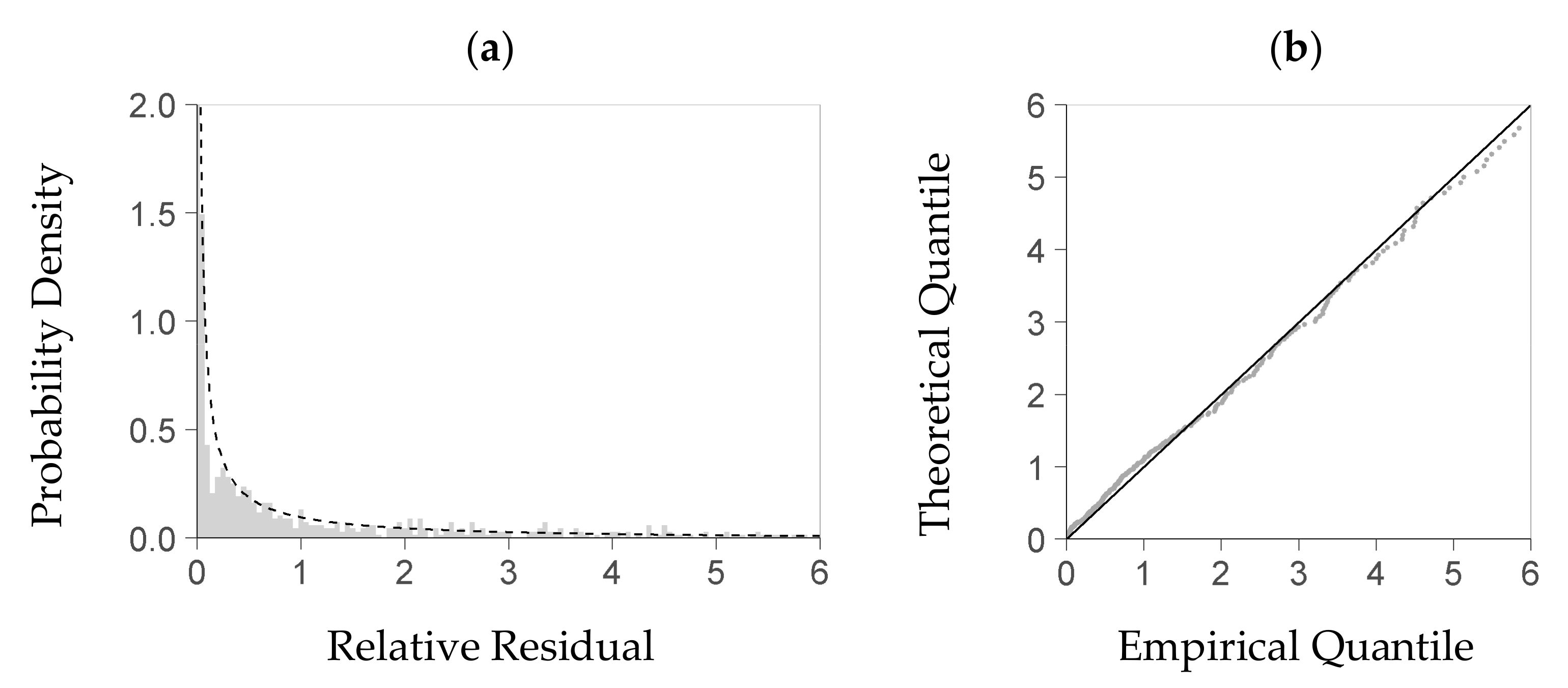
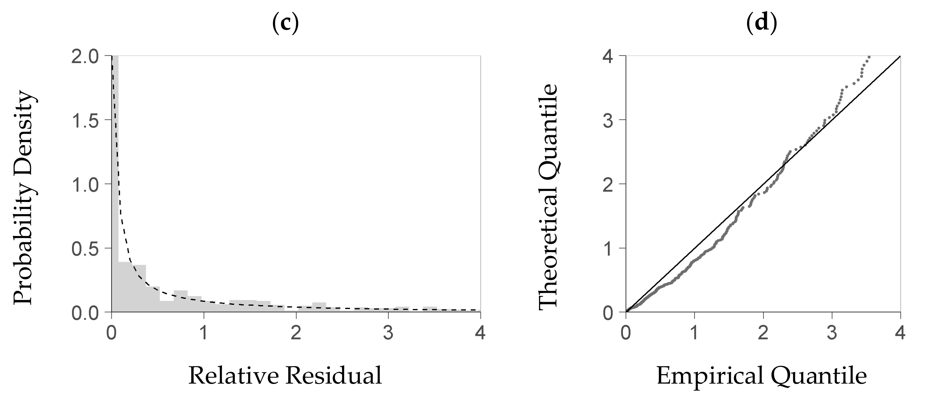
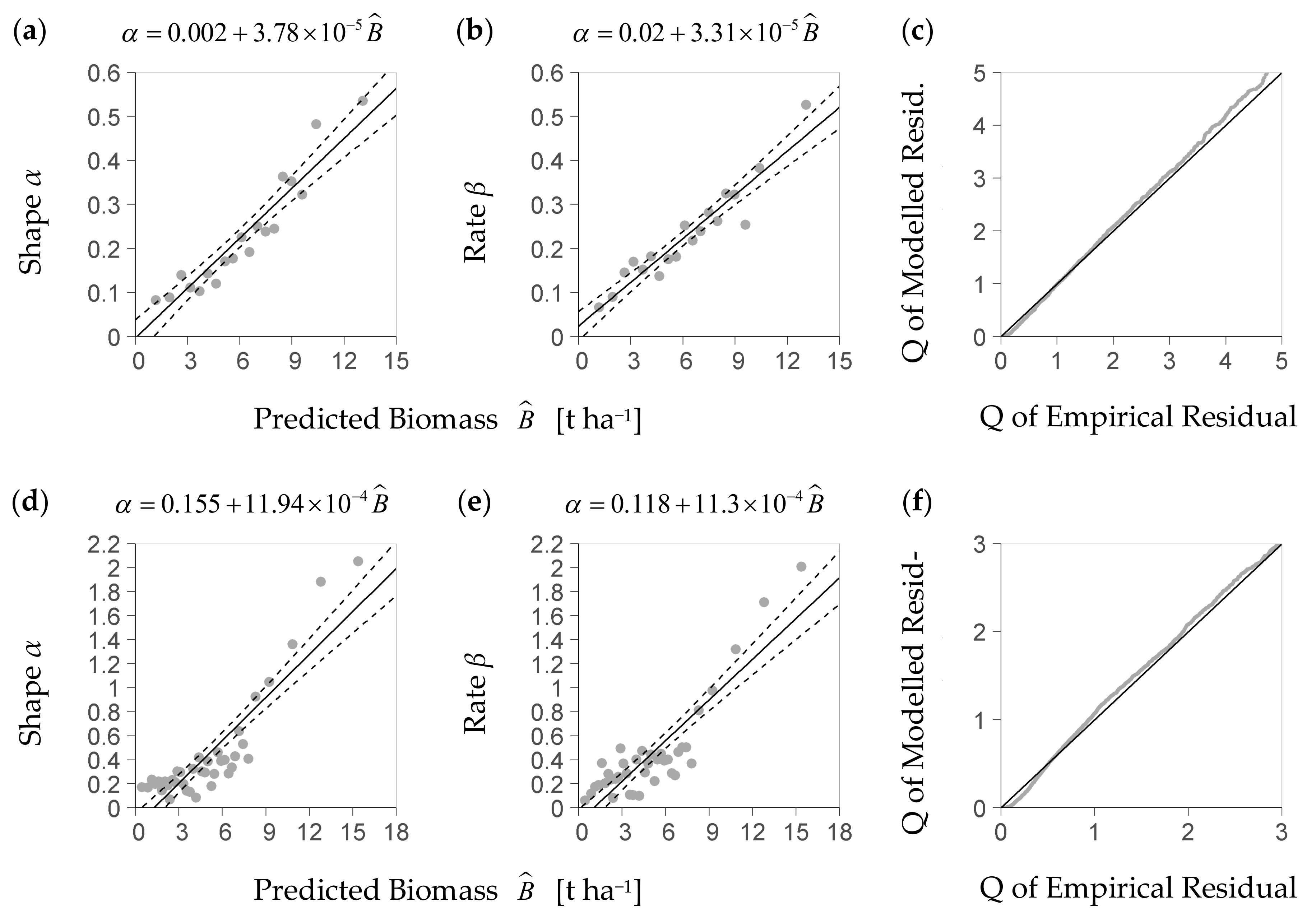
Within the predictors’ center range considered for distribution analysis (see Section 2.4), given now by intervals of Dq, Hmax, and SDI, the KS-test rejected the strict hypothesis that the gamma probability density function was a precise theoretical model of the residuals’ distribution. A QQ-plot, however, indicates (Figure 3b,d) that this density function is a feasible approximation to the empirical density distribution of the residuals (Figure 3a,c). If estimated from the deterministic part of the NFI-based model and its residuals, the relation between the predicted biomass and each parameter of the gamma density function, shape and rate, is close to a linear one (Figure 4a,b). A linear trend also sufficiently approximates both relations if they are based on the BSFI data and the deterministic part of the BSFI-based model (Figure 4d,e). Sampling from the stochastic parts of both models (as described in Section 2.4), within at least 95% of the data, yielded a distribution that had similar quantiles as the one computed from observed residuals (QQ-plot, Figure 4c,f).
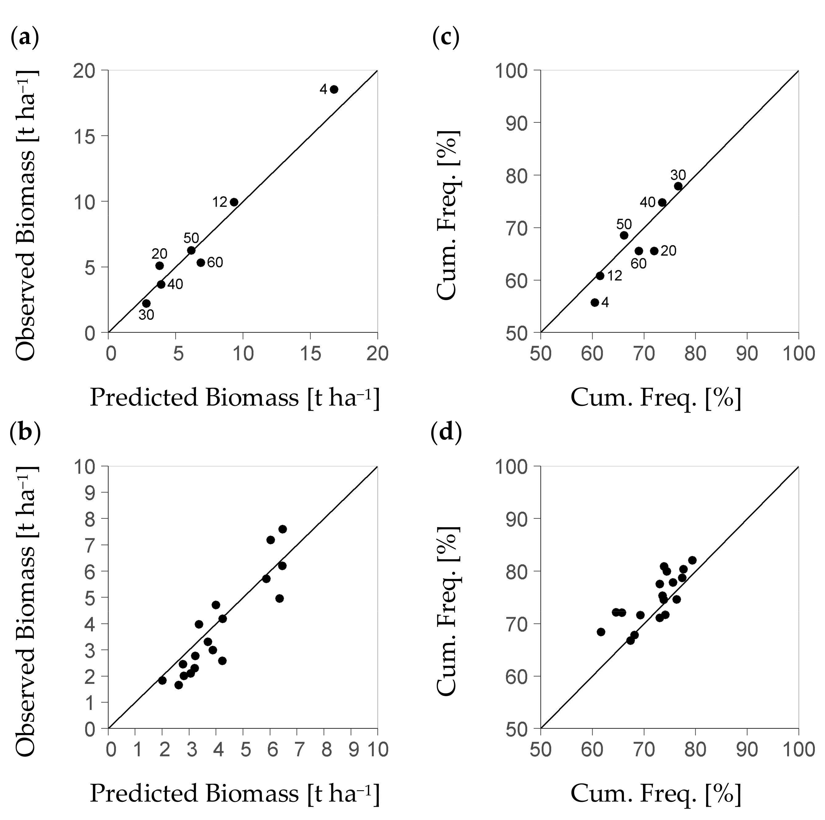
Further results consider the evaluation of the BSFI-based model as dependent on the level of stratum differentiation, i.e., on the degree of landscape discretization. The basic stratification that only used the criterion of diameter class (Table 3) formed a set of seven strata. Among these strata, the ratio of measured to modelled regeneration biomass had a mean of one-fold (Figure 5a). It ranged from 0.8 to 1.2-fold. Among the diameter classes 30, 40, and 50 that represent 71% of all 11,954 BSFI plots used, the bias range was notably smaller, i.e., from 0.8 to 1.0-fold. Cumulative frequency values (%) based on measured data deviated from the predicted ones by absolute values ranging from −7.4 to 2.6 (Figure 5c). Among strata of classes 30, 40, and 50 (Table 3), again, the absolute deviation of measured from modelled cumulative frequency (%) was small at a maximum of ±0.6.
The stratification resulted in a notably smaller plot number per stratum, if it was based on the forest management unit in addition to the diameter class. Then, exclusively strata of diameter classes 30, 40, and 50 provided the minimum sample size postulated by the study at hand (140 plots). Only such strata will be considered by the following analysis. Still, they comprise 71% of all plots from the BSFI data set. The range of bias between measured and predicted per-stratum mean biomass among strata of that group was notably higher than the typical one among such strata that were based on the diameter class only. Their bias range was from 0.6 to 1.2-fold vs. 0.8 to 1.0-fold. The bias had a mean of 0.9-fold (Figure 5b vs. a). Thus, there was an additional bias of predicted stratum biomass within ±0.2-fold, if the strata formation used the forest management unit as a further criterion. That additional data spread was due to the scatter of the observed per-stratum values around their diameter-class average (±0.15-fold).
Moreover, there was also an increase of the absolute deviation in the mean’s cumulative frequency (%), related to the forest management unit level, which was at ±6. Hence, there was a notable stochastic effect on the forest management unit-level that reduced the precision of the model, if strata were formed by both diameter class and forest management unit. All stratum-related values that we presented here are stable: the uncertainty of any observed average value per stratum due to per plot variation of regeneration biomass was commonly below 0.05-fold of the observed value.
4. Discussion
4.1. The Study Responds to a Common Requirement for Model Initialization
Regeneration constitutes a key process within the development of forest structure and stock [40]. Its initial state is thus a pivotal condition for the result of forest management scenarios that exemplify the development of ecosystem services on the landscape scale level (e.g., [1]). In order to estimate regeneration within the northern Rocky Mountains, Ferguson et al. [41] predicted the probability per tree density class and the maximum tree height among regeneration trees with a statistical model obtained from stand management lists. Schweiger and Sterba [11], as well as Tremer et al. [12], extended that approach in order to represent the tree density per species and height class. Kolo et al. [13], based on the German national forest inventory, presented a model that estimates the probability of regeneration to occur based on German national forest inventory data. They underpin the relevance of structure and site as model predictors.
Biomass growth is closely linked to the stand intrinsic fluxes of radiation, heat, and water. These fluxes, in turn, depend on resistances that originate from canopy and soil properties [42]. Regeneration biomass thus represents a fundamental outcome of the regeneration process. On the experimental plot level, that key variable has enabled researchers to survey the quantitative relation of regeneration stock and structural indicators [29]. The study at hand considers a continuative approach in order to represent regeneration stock on the landscape scale level. It aims to supplement virtual stands from simulation strata with a realistic amount of regeneration biomass. The rationale for using biomass as a predicted variable is to split up the modelling of regeneration stock into two consecutive steps. The first step is the estimation of regeneration biomass involving an essential stochastic component that accounts for previous and unrecorded disturbances. The second one is yet to be implemented. It distributes the biomass estimated per tile of a dynamic regeneration model among tree size classes. In order to initialize dynamic models, we will complement our approach by an algorithm that derives the species-specific proportion of regeneration biomass. Therefore, a logistic model (e.g., as used by Tremer et al. [12]) based on overstory species shares is a likely candidate. Moreover, our model type will translate regeneration biomass into a realistic height profile of tree density. That profile will likely be based on a biomass-related maximum height per plot and a tree biomass to height relation from empirical data.
4.2. The Study Conceptualizes and Evaluates a Novel Biomass-Based Approach
The statistical model from the study at hand comprised a deterministic part and a stochastic one. Both parts complement each other in order to predict the characteristic distribution of regeneration biomass within plot-sized stratum subsectors. Within the deterministic module, we aimed to reduce the number of presumptions on the one hand and the degrees of freedom on the other. Therefore, we applied a linear relationship between the biomass and most of the predictors considered. In order to represent the dependence of regeneration biomass on the Dq, however, we presumed a nonlinear partial regression. The results confirmed that nonlinear relationship and showed that Dq is a highly relevant predictor. Kolo et al. [13] underpinned that relevance and reported an increase of probability with Dq. However, they pointed to the converse trend within previous work. The study at hand demonstrated that both tendencies exist and depend on stand maturity. Moreover, the deterministic part of the NFI-based model points to a local maximum of biomass at a Dq of 50 cm. The strong increase of regeneration stock with lower Dq values starting from 35 cm is likely due to target diameter felling and the removal of competitors within the overstory. An indicated drop of the biomass at Dq values beyond the local maximum is well justified by a decreasing abundance of mature beech [43].
An observed value of regeneration biomass, beyond resource supply to the understory, may imply both intensity and point in time of a disturbance. Disturbance incidents are rarely reported within inventory data. However, they influence the residual distribution of regeneration biomass at given predictor values. Therefore, we complemented the deterministic model part with a stochastic one that describes the distribution of relative residuals. That stochastic model part used the gamma probability density function. After parameterization, that variable shape function strictly monotonically decreased with pole zero and asymptote zero. Previous work [44,45] has reported a distribution of canopy gap size that resembles a falling exponential function. It underpins that the gamma density distribution function is a suitable approximation to the regeneration biomass distribution at given overstory structure attributes. Although the model type of the study at hand is suitable for both of the inventories considered, the NFI-based model, as it has the more general geographical scope, is the actual candidate of further development.
4.3. The Modelling Approach Exemplified Provides a Basis of Future Development
We exemplarily evaluated the predictive quality of the model type presented as dependent on the stratum resolution. Therefore, we applied the BSFI-based model, in a first step, to strata that exclusively differ in the average diameter of their inventory plots. That application test underpinned that a regeneration biomass model of the type considered may sufficiently approximate the regeneration biomass of such generalist strata. Moreover, the model met the observed cumulative frequency of the average biomass per stratum. The stochastic part of the model thus generated a realistic heterogeneity of the stratum-intrinsic regeneration biomass. However, a test with strata of a higher discretization level that also included the forest management unit was linked to a notable increase of model bias. That additional bias was certainly due to processes that, on the one hand, vary among strata with size of a forest management unit but, on the other, have no equivalents in the model as fixed effects.
4.4. Browsing Is a Likely Missing Indicator
Kupferschmid et al. [19] pointed out that browsing intensity considerably varies among Swiss federal states (Kanton), many of which have a total area of about 150,000 ha. That area size corresponds to the average size of the total landscape around a typical German state forest management unit. Browsing in general has been reported to be a severe inhibitor of regeneration [46,47,48]. Kolo et al. [13] accordingly assumed that browsing is a major cause of leeway within their prediction of regeneration probability.
4.5. Most of the Random Effect Is Due to Within-Stand Variability
Kolo et al. [13] reported that their model predicts the occurrence of regeneration at a notably high rate of 72%. The remaining leeway of 28% corresponds to the wide probability distribution within the stochastic part of both our models. The variation among forest management unit-based strata, in contrast to that among plots, was notably smaller. That finding indicates that even at the highest discretization level considered, the largest part of variability is intrinsic to each stratum. Thus, the stochastic model part, as given by the residual distribution of the deterministic part, mostly represented a typical stand-intrinsic variation. Hence, one may consider its distribution characteristics as mainly governed by small-scale effects.
4.6. Application of Such Model Has to Account for General Limitations of Any Inventory
A study on inventory plots cannot guarantee that the overstory recorded within a plot is equivalent to the one that takes influence on the plot’s regeneration (light from aside [49]). Within the NFI data, an error due to side light effects is less critical, as the small inventory circle for regeneration is situated five meters north of the plot center. Moreover, the radius of angle count sampling increases with DBH and hence canopy height (e.g., at DBH 40 cm to 20 m). Thus, the overstory fraction that controls the influence of direct solar irradiance is likely covered by the inventory method of the NFI to the largest part.
4.7. The Most Relevant Predictors Will Be Accessible through Remote Sensing
The ongoing development of airborne laser scanning (ALS) contributes novel methods for the collection and analysis of 3D point clouds. Such methods permit researchers to access crown diameters and to classify tree species below the top-most layer of a stand, as exemplified by Lindberg and Holmgren [50]. Jucker et al. [51] presented allometric equations that infer the tree diameter from airborne crown dimensions. The most relevant indicators of our model, Dq, Hmax, and SDI, will thus be a regular future outcome of remote sensing-based inventories. ALS, moreover, may gain support through combination with further airborne and terrestrial methods, such as Terrestrial Laser Scanning (TLS) [52].
4.8. Future Work Has to Explain Random Effects and Might Extend the Focus of Model Application
The most relevant task of future development is to identify the processes that explain the model bias on the level of a forest management unit. A possible one is browsing that is strongly related to the local hunting regime [53]. Further research has to quantify the intensity of such processes by predictor variables that are available from local forest management, e.g., as class variables. If one applies the model to inventories that cover multiple tenure types, the model quality will certainly benefit from including the type of the forest owner [13]. Statistical regeneration models might further be used to support the plausibility of spin-up runs. Such dynamic initializations are well established for defining the initial regeneration status within succession models, e.g., in [54]. A statistical regeneration model, moreover, might be applied to correct values of regeneration stock after several time steps of a simulation have passed.
5. Conclusions
The study’s type of regeneration model significantly relates regeneration biomass to indicators of structure and site. Within large subunits of forest landscape classified by dominating species and average diameter, such a model represents regeneration stock at an acceptable precision. For initializing dynamic management scenarios on the landscape scale level, the approach is thus promising. However, this type of model requires additional indicators, if the landscape subunits also differ by the forest management unit. One possible candidate for such a predictor is browsing.
The Quadratic Mean Diameter (Dq) is a strong indicator of stand development and, moreover, of regeneration biomass. An average tree diameter is thus a well-reasoned stratification criterion. Dq, Hmax, and SDI are the most relevant predictors. This finding is promising for a remote detection of key stand attributes. Future development of the statistical regeneration model will consider browsing as an additional predictor. Therefore, a quantitative relation between browsing intensity and regeneration stock within inventory data will be advantageous. The modelling approach, as a future benefit, may help to estimate the potential of natural forest recovery after severe overstory loss.
Acknowledgments
The authors wish to express their gratitude to the Bayerische Staatsforsten AÖR, Regensburg (BaySF) for providing valuable data from their regular inventories. Special thanks are also due to the Thünen Institut Eberswalde for supplying national forest inventory data. In particular, we would like to thank Thomas Riedel (Thünen Institut) for consultancy in biomass computation, biomass extraction, and overstory structure extraction from the public database. The authors wish to thank Rüdiger Grote, Michael Heym, Torben Hilmers, Ralf Moshammer, Leonhard Steinacker, and Enno Uhl for inspiration and discussion. Special thanks are due to the European Union for support of this study through funding of (1) project ALTERFOR within the Horizon 2020 research and innovation programme under grant agreement No 676754 and of (2) project ClusterWIS within the European Regional Development fund under grant aggreement EFRE-080003 (EFRE.NRW 2014-2020). Online publication of his work was supported by the German Research Foundation (DFG) and the Technical University of Munich within the funding programme Open Access Publishing.
Author Contributions
Werner Poschenrieder conceptualized the model, the data preparation, the model calibration, the model evaluation, and the article’s structure. Werner Poschenrieder conducted all practical work of modelling and data handling and wrote the paper. Peter Biber gave specialist advice in statistical modelling and evaluation. Peter Biber reviewed the paper and contributed to all sections through editing. Hans Pretzsch supervised and reviewed the study and gave profound expert advice in regeneration dynamics.
Conflicts of Interest
The authors declare no conflict of interest.
Appendix A
An allometric height-diameter model was fitted to to overstory tree height and diameter. That model followed Equation (A1):
where h and d are individual tree height and diameter, respectively, and A and B are parameters. That model was fitted to individual tree overstory data from the deciduous fraction of the NFI to meet the conditional (1) mean value; (2) 2.5% quantile; and (3) 97.5% quantile of height h as dependent on diamteter d. Thus, we obtained three representations of Equation (A1) with defined parameter values (Table A1) that enabled us to represent a conditional gaussian distribution of h at any given diamteter d. That conditional gaussian distribution enabled us to calculate the Height Diameter Characteristic given by Equation (A2) as a conditional probability P:
where h is height as a random variable, d is DBH as a predictor, and h0 and d0 are tree height and DBH as measured, respectively.

Table A1.
Parameter values that result from fitting of Equation (A1) to the distribution of individual tree height–diameter data.
Table A1.
Parameter values that result from fitting of Equation (A1) to the distribution of individual tree height–diameter data.
| Distribution Characteristic Equation (A1) Was Fitted to | Parameter Value | |
|---|---|---|
| A | B | |
| Mean | 5.142 | 0.437 |
| 2.5% quantile | 1.803 | 0.580 |
| 97.5% quantile | 7.563 | 0.420 |
Appendix B
In order to assess the importance of each individual predictor, we removed each predictor variable exclusively from the model of minimum AIC to obtain one nested model per predictor removed. We then compared the AIC value of that nested sub model to the AIC value of the optimal one. That variable whose exclusion caused the greatest AIC difference was considered the most important one.
Appendix C
Two polynomials were applied in order to approximate the spline s(Dq) within the deterministic part of both the NFI-based model (Equation (4a)) and the BSFI-based model (Equation (4b)). They enable the application of each model independently of the original data and of the statistical software R. Each polynomial conforms to the following Equation (A3):
where ΔB is the change in regeneration biomass related to Dq. That approximation may be applied in order to predict biomass from Dq and each remainder predictor (see Equations (4a) resp. (4b)). To that end, first the corresponding row in Table A2(NFI) and Table A3 (BSFI) is to be selected. The row to be considered is the one with the Dq interval that encloses the given value of Dq. The approximate value of predicted regeneration biomass B is then:
where I is the value in the column Intercept of the table considered; S is the sum of each of the predictors except Dq multiplied by the slope given with its name; and ΔB is the value that results from applying Equation (A3) to Dq and the parameters from columns d1, d2, and d3. Each of these approximations is exclusively valid within the corresponding interval of Dq (hence, the intercepts may notably differ).
Table A2.
The parameters of the approximation to the deterministic part of the NFI-based model (see Section 2.3 and Equation (A3)) that substitutes s(Dq) by two polynomials; the intercept implies that of the polynomial approximation and thus depends on the interval of Dq.
Table A2.
The parameters of the approximation to the deterministic part of the NFI-based model (see Section 2.3 and Equation (A3)) that substitutes s(Dq) by two polynomials; the intercept implies that of the polynomial approximation and thus depends on the interval of Dq.
| Dq Interval | Intercept | Slope of | |||||||
|---|---|---|---|---|---|---|---|---|---|
| SDI | SPI | SI | Hmax | HD | d1 | d2 | d3 | ||
| ≤56.6 | 79,000 | −6.87 | −1498 | −1304 | 304 | −2927 | −2543 | 66.88 | −0.54 |
| >56.6 | 52,630 | −6.87 | −1498 | −1304 | 304 | −2927 | −2.06 | −0.58 | 0 |
Table A3.
The parameters of the approximation to the deterministic part of the BSFI-based model (see Section 2.3 and Equation (A3)) that substitutes s(Dq) by two polynomials; the intercept implies that of the polynomial approximation and thus depends on the interval of Dq.
Table A3.
The parameters of the approximation to the deterministic part of the BSFI-based model (see Section 2.3 and Equation (A3)) that substitutes s(Dq) by two polynomials; the intercept implies that of the polynomial approximation and thus depends on the interval of Dq.
| Dq Interval | Intercept | Slope of | |||||||
|---|---|---|---|---|---|---|---|---|---|
| SDI | SPI | SI | Hmax | HD | d1 | d2 | d3 | ||
| ≤35 | 50,530 | 40,074 | −4.59 | −1194 | -- | 255 | 1338 | −19.06 | 0.082 |
| >35 | −25,973 | 40,074 | −4.59 | −1194 | -- | 255 | −5522 | 206 | −2.55 |
References
- Biber, P.; Borges, J.; Moshammer, R.; Barreiro, S.; Botequim, B.; Brodrechtová, Y.; Brukas, V.; Chirici, G.; Cordero-Debets, R.; Corrigan, E.; et al. How Sensitive Are Ecosystem Services in European Forest Landscapes to Silvicultural Treatment? Forests 2015, 6, 1666–1695. [Google Scholar] [CrossRef]
- Jonsson, B.; Jacobsson, J.; Kallur, H. The Forest Management Planning Package Theory and Application. Stud. For. Suec. 1993, 189, 1–56. [Google Scholar]
- Pott, M.; Fabrika, M. An Information System for the Evaluation and Spatial Analysis of Forest Inventory Data. Forstwiss. Cent. 2002, 121 (Suppl. 1), 80–88. [Google Scholar]
- Pretzsch, H. Forest Dynamics, Growth and Yield; Springer: Berlin/Heidelberg, Germany, 2009; ISBN 978-3-540-88306-7. [Google Scholar]
- Canadian Forest Inventory Committee. Canada’s National Forest Inventory Ground Sampling Guidelines: Specifications for Ongoing Measurement; Natural Resources Canada, Canadian Forest Service, Pacific Forestry Centre: Victoria, BC, Canada, 2008.
- Polley, H. Survey Instructions for the 3rd National Forest Inventory (2011–2012) 2nd Revised Version, May 2011 with 4. Corrigendum (21.03.2014); Bundesministerium für Ernährung, Landwirtschaft und Verbraucherschutz Ref. 535; Federal Ministry of Food, Agriculture, and Consumer Protection: Bonn, Germany, 2011. [Google Scholar]
- Hunziker, U.; Brang, P. Microsite Patterns of Conifer Seedling Establishment and Growth in a Mixed Stand in the Southern Alps. For. Ecol. Manag. 2005, 210, 67–79. [Google Scholar] [CrossRef]
- Abdullahi, S.; Kugler, F.; Pretzsch, H. Prediction of stem volume in complex temperate forest stands using TanDEM-X SAR data. Remote Sens. Environ. 2016, 174, 197–211. [Google Scholar] [CrossRef]
- Abdullahi, S.; Schardt, M.; Pretzsch, H. An unsupervised two-stage clustering approach for forest structure classification based on X-band InSAR data. A case study in complex temperate forest stands. Int. J. Appl. Earth Obs. Geoinf. 2017, 57, 36–48. [Google Scholar] [CrossRef]
- Kayitakire, F.; Hamel, C.; Defourny, P. Retrieving forest structure variables based on image texture analysis and IKONOS-2 imagery. Remote Sens. Environ. 2006, 102, 390–401. [Google Scholar] [CrossRef]
- Schweiger, J.; Sterba, H. A Model Describing Natural Regeneration Recruitment of Norway Spruce (Picea abies (L.) Karst.) in Austria. For. Ecol. Manag. 1997, 97, 107–118. [Google Scholar] [CrossRef]
- Tremer, N.; Schmidt, M.; Hansen, J. Estimating the Structure of Natural Regeneration Based on Inventory Data. Allg. Forst Jagdztg. 2005, 176, 1–13. [Google Scholar]
- Kolo, H.; Ankerst, D.; Knoke, T. Predicting Natural Forest Regeneration: A Statistical Model Based on Inventory Data. Eur. J. For. Res. 2017, 136, 923–938. [Google Scholar] [CrossRef]
- Lutze, M.; Ades, P.; Campbell, R. Spatial Distribution of Regeneration in Mixed-Species Forests of Victoria. Aust. For. 2004, 67, 172–183. [Google Scholar] [CrossRef]
- Gravel, D.; Beaudet, M.; Messier, C. Partitioning the Factors of Spatial Variation in Regeneration Density of Shade-Tolerant Tree Species. Ecology 2008, 89, 2879–2888. [Google Scholar] [CrossRef] [PubMed]
- Pretzsch, H.; Biber, P.; Ďurský, J. The Single Tree-Based Stand Simulator SILVA: Construction, Application and Evaluation. For. Ecol. Manag. 2002, 162, 3–21. [Google Scholar] [CrossRef]
- Seidl, R.; Lexer, M.J.; Jager, D.; Honninger, K. Evaluating the Accuracy and Generality of a Hybrid Patch Model. Tree Physiol. 2005, 25, 939–951. [Google Scholar] [CrossRef] [PubMed]
- Fischer, R.; Bohn, F.; Dantas de Paula, M.; Dislich, C.; Groeneveld, J.; Gutiérrez, A.G.; Kazmierczak, M.; Knapp, N.; Lehmann, S.; Paulick, S.; et al. Lessons Learned from Applying a Forest Gap Model to Understand Ecosystem and Carbon Dynamics of Complex Tropical Forests. Ecol. Model. 2016, 326, 124–133. [Google Scholar] [CrossRef] [Green Version]
- Kupferschmid, A.D.; Heiri, C.; Huber, M.; Fehr, M.; Frei, M.; Gmür, P.; Imesch, N.; Zinggeler, J.; Brang, P.; Clivaz, J.C.; et al. Einfluss Wildlebender Huftiere Auf Die Waldverjüngung: Ein Überblick Für Die Schweiz. Schweiz. Z. Forst. 2015, 166, 420–431. [Google Scholar] [CrossRef]
- Clark, D.A.; Brown, S.; Kicklighter, D.W.; Chambers, J.Q.; Thomlinson, J.R.; Ni, J. Measuring Net Primary Production in Forest Concepts and Field Methods. Ecol. Appl. 2001, 11, 356–370. [Google Scholar] [CrossRef]
- Thünen Institute, Germany. German National Forest Inventory (BWI) Results Database. Available online: https://bwi.info (accessed on 1 September 2015).
- Kändler, G.; Bösch, B. Überprüfung und Neukonzeption einer Biomassefunktion. Abschlussbericht 2b; Abt. Biometrie und Informatik Wonnhaldestraße 4 79100; Forstliche Versuchs- und Forschungsanstalt Baden-Württemberg: Freiburg, Germany, 2013. [Google Scholar]
- Röhling, S.; Dunger, K.; Kändler, G.; Klatt, S.; Riedel, T.; Stümer, W.; Brötz, J. Comparison of Calculation Methods for Estimating Annual Carbon Stock Change in German Forests under Forest Management in the German Greenhouse Gas Inventory. Carbon Balance Manag. 2016, 11, 12. [Google Scholar] [CrossRef] [PubMed]
- Marklund, L.G. Biomass Functions for Norway Spruce (Picea abies (L.) Karst) in Sweden; SLU, Swedish University of Agricultural Sciences, Department of Forest Survey: Uppsala, Sweden, 1987. [Google Scholar]
- Neufanger, M.; Faltl, W.; Schelhaas, C. Anleitung zur Durchführung von Betriebsinventuren in den Bayerischen Staatsforsten. FE AA 010 Durchführung von Betriebsinventuren; Bayerische Staatsforsten AöR: Munich, Germany, 2012. [Google Scholar]
- Kozlowski, T.T. Physiological Ecology of Natural Regeneration of Harvested and Disturbed Forest Stands: Implications for Forest Management. For. Ecol. Manag. 2002, 158, 195–221. [Google Scholar] [CrossRef]
- Pardos, M.; Montero, G.; Cañellas, I.; Ruiz del Castillo, J. Ecophysiology of Natural Regeneration of Forest Stands in Spain. For. Syst. 2005, 14, 434–445. [Google Scholar] [CrossRef]
- Reineke, L.H. Perfecting a stand-density index for even-aged forests. J. Agric. Res. 1933, 46, 627–638. [Google Scholar]
- Pretzsch, H.; Biber, P.; Uhl, E.; Dauber, E. Long-Term Stand Dynamics of Managed Spruce-Fir-Beech Mountain Forests in Central Europe: Structure, Productivity and Regeneration Success. Forestry 2015, 88, 407–428. [Google Scholar] [CrossRef]
- Thünen Institute, Germany. Digital Map of Forest Ecological Regions (Wuchsgebiete/Wuchsbezirke). Available online: https://gdi.thuenen.de/wo/wgwb/ (accessed on 1 September 2015).
- Wood, S.N. Generalized Additive Models: An Introduction with R, 2nd ed.; Chapman and Hall/CRC Press; Taylor Francis Inc.: New York, NY, USA, 2017; ISBN 978-1-49-872833-1. [Google Scholar]
- Fahrmeir, L.; Kneib, T.; Lang, S.; Marx, B. Extensions of the Classical Linear Model. In Regression; Springer: Berlin/Heidelberg, Germany, 2013; pp. 177–267. ISBN 978-3-642-34332-2. [Google Scholar]
- R Core Team. R: A Language and Environment for Statistical Computing; R Foundation for Statistical Computing: Vienna, Austria, 2016; Available online: https://www.R-project.org/ (accessed on 24 April 2016).
- Wood, S.; Scheipl, F. Gamm4: Generalized Additive Mixed Models Using ‘mgcv’ and ‘lme4’. R Package Version 0.2-5. Available online: https://CRAN.R-project.org/package=gamm4 (accessed on 25 November 2017).
- Delignette-Muller, M.L.; Dutang, C. fitdistrplus: An R Package for Fitting Distributions. J. Stat. Softw. 2015, 64, 1–34. Available online: http://www.jstatsoft.org/v64/i04/ (accessed on 24 April 2016). [CrossRef]
- Akaike, H. Prediction and Entropy. In A Celebration of Statistics; Atkinson, A.C., Fienberg, S.E., Eds.; Springer: New York, NY, USA, 1985; pp. 1–24. [Google Scholar]
- Marsaglia, G.; Tsang, W.W.; Wang, J. Evaluating Kolmogorov’s distribution. J. Stat. Softw. 2003, 8. Available online: http://www.jstatsoft.org/v08/i18/ (accessed on 24 April 2016). [CrossRef]
- Becker, R.A.; Chambers, J.M.; Wilks, A.R. The New S Language; Chapman & Hall/CRC: London, UK, 1988; ISBN 978-0-534-09192-7. [Google Scholar]
- Efron, B. Bootstrap Methods: Another Look at the Jackknife. Ann. Stat. 1979, 7, 1–26. [Google Scholar] [CrossRef]
- Price, D.T.; Zimmermann, N.E.; van der Meer, P.J.; Lexer, M.J.; Leadley, P.; Jorritsma, I.T.M.; Schaber, J.; Clark, D.F.; Lasch, P.; McNulty, S.; et al. Regeneration in Gap Models: Priority Issues for Studying Forest Responses To Climate Change. Clim. Chang. 2001, 51, 475–508. [Google Scholar] [CrossRef]
- Ferguson, D.E.; Carlson, C.E. Predicting Regeneration Establishment with the Prognosis Model; No. 467, 1-U54; Forest Service: Ogden, UT, USA, 1993. [Google Scholar]
- Landsberg, J.J.; Waring, R.H. A Generalised Model of Forest Productivity Using Simplified Concepts of Radiation-Use Efficiency, Carbon Balance and Partitioning. For. Ecol. Manag. 1997, 95, 209–228. [Google Scholar] [CrossRef]
- Barna, M. The Effects of Cutting Regimes on Natural Regeneration in Submountain Beech Forests: Species Diversity and Abundance. J. For. Sci. 2008, 54, 533–544. [Google Scholar] [CrossRef]
- Foster, J.R.; Reiners, W.A. Size Distribution and Expansion of Canopy Gaps in a Northern Appalachian Spruce-Fir Forest. Vegetatio 1986, 68, 109–114. [Google Scholar]
- Asner, G.P.; Kellner, J.R.; Kennedy-Bowdoin, T.; Knapp, D.E.; Anderson, C.; Martin, R.E. Forest Canopy Gap Distributions in the Southern Peruvian Amazon. PLoS ONE 2013, 8, e60875. [Google Scholar] [CrossRef] [PubMed]
- Ammer, C. Impact of Ungulates on Structure and Dynamics of Natural Regeneration of Mixed Mountain Forests in the Bavarian Alps. For. Ecol. Manag. 1996, 88, 43–53. [Google Scholar] [CrossRef]
- Motta, R. Impact of Wild Ungulates on Forest Regeneration and Tree Composition of Mountain Forests in the Western Italian Alps. For. Ecol. Manag. 1996, 88, 93–98. [Google Scholar] [CrossRef]
- Boulanger, V.; Baltzinger, C.; Saïd, S.; Ballon, P.; Picard, J.F.; Dupouey, J.L. Ranking Temperate Woody Species along a Gradient of Browsing by Deer. For. Ecol. Manag. 2009, 258, 1397–1406. [Google Scholar] [CrossRef]
- Golser, M.; Hasenauer, H. Predicting Juvenile Tree Height Growth in Uneven-Aged Mixed Species Stands in Austria. For. Ecol. Manag. 1997, 97, 133–146. [Google Scholar] [CrossRef]
- Lindberg, E.; Holmgren, J. Individual Tree Crown Methods for 3D Data from Remote Sensing. Curr. For. Rep. 2017, 3, 19–31. [Google Scholar] [CrossRef]
- Jucker, T.; Caspersen, J.; Chave, J.; Antin, C.; Barbier, N.; Bongers, F.; Dalponte, M.; van Ewijk, K.Y.; Forrester, D.I.; Haeni, M.; et al. Allometric Equations for Integrating Remote Sensing Imagery into Forest Monitoring Programmes. Glob. Chang. Biol. 2017, 23, 177–190. [Google Scholar] [CrossRef] [PubMed]
- Hyyppä, J.; Hyyppä, H.; Leckie, D.; Gougeon, F.; Yu, X.; Maltamo, M. Review of Methods of Small-footprint Airborne Laser Scanning for Extracting Forest Inventory Data in Boreal Forests. Int. J. Remote Sens. 2008, 29, 1339–1366. [Google Scholar] [CrossRef]
- Hothorn, T.; Müller, J. Large-Scale Reduction of Ungulate Browsing by Managed Sport Hunting. For. Ecol. Manag. 2010, 260, 1416–1423. [Google Scholar] [CrossRef]
- Didion, M.; Kupferschmid, A.D.; Bugmann, H. Long-Term Effects of Ungulate Browsing on Forest Composition and Structure. For. Ecol. Manag. 2009, 258, 44–55. [Google Scholar] [CrossRef]
Figure 1.
Profiles of regeneration biomass as predicted by the deterministic model part based on the NFI (German National Forest Inventory, Equation (4a)). Each profile is presented over one predictor with, at the same time, the remainder predictors at their mean value (abbreviation H-D: Height-Diameter); profiles ordered by the relevance of the referring predictor based on the AIC criterion ((a–f), see Section 2.4); dotted lines refer to the confidence interval; each predictor shown within its 95% interval; the stochastic part (Figure 3a,b) covers the residual distribution.
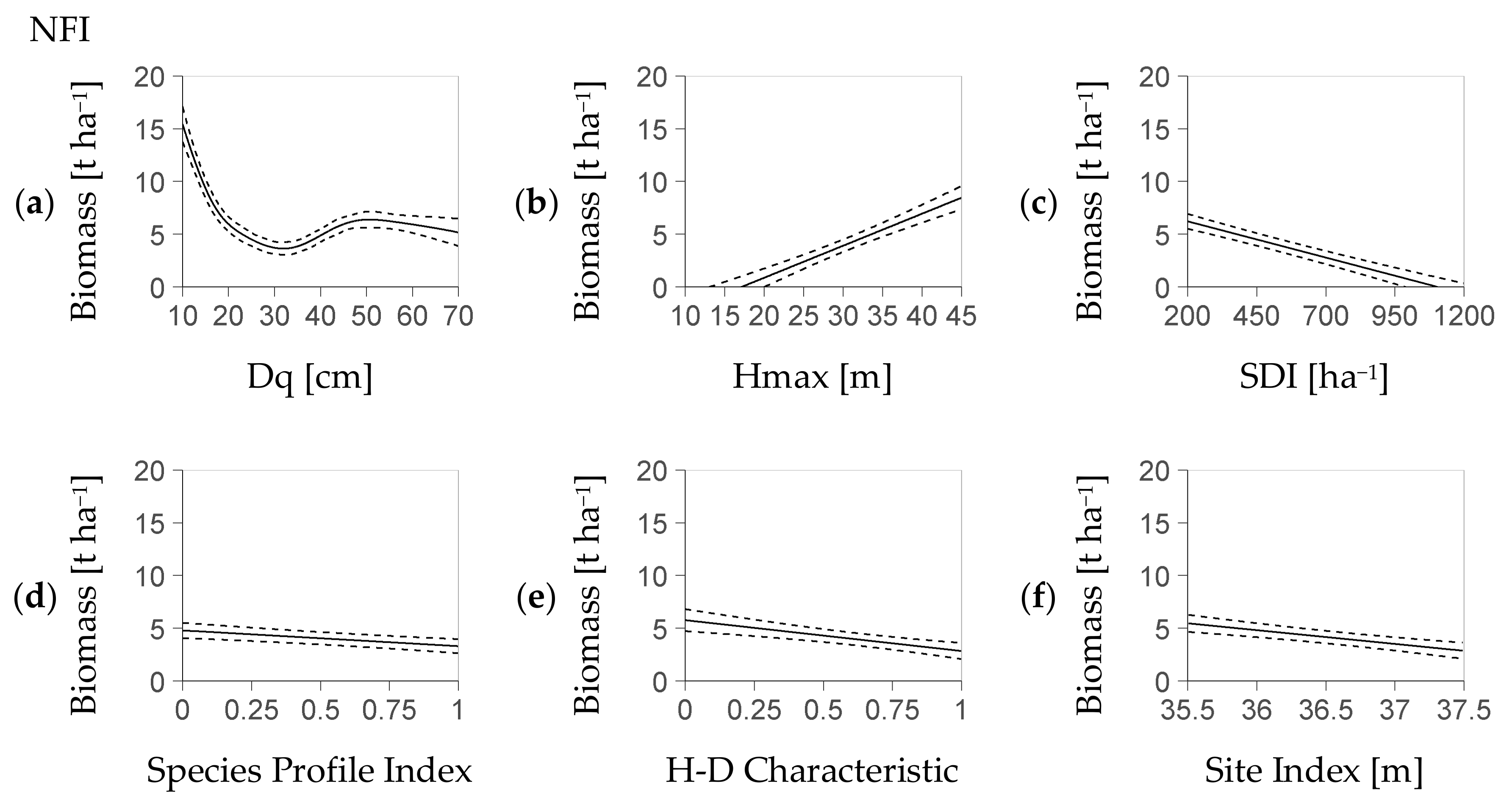
Figure 2.
Profiles of regeneration biomass as predicted by the deterministic model part based on the BSFI (Bavarian State Forest Inventory, Equation (4b)). Each profile is presented over one predictor with, at the same time, the remainder predictors at their mean value (abbreviation H-D: Height-Diameter); profiles ordered by the relevance of the referring predictor based on the AIC criterion ((a–e), see Section 2.4); dotted lines refer to the confidence interval; each predictor shown within its 95% interval; the stochastic part (Figure 3c,d) covers the residual distribution (profiles based on 5881 BSFI plots used for model calibration).
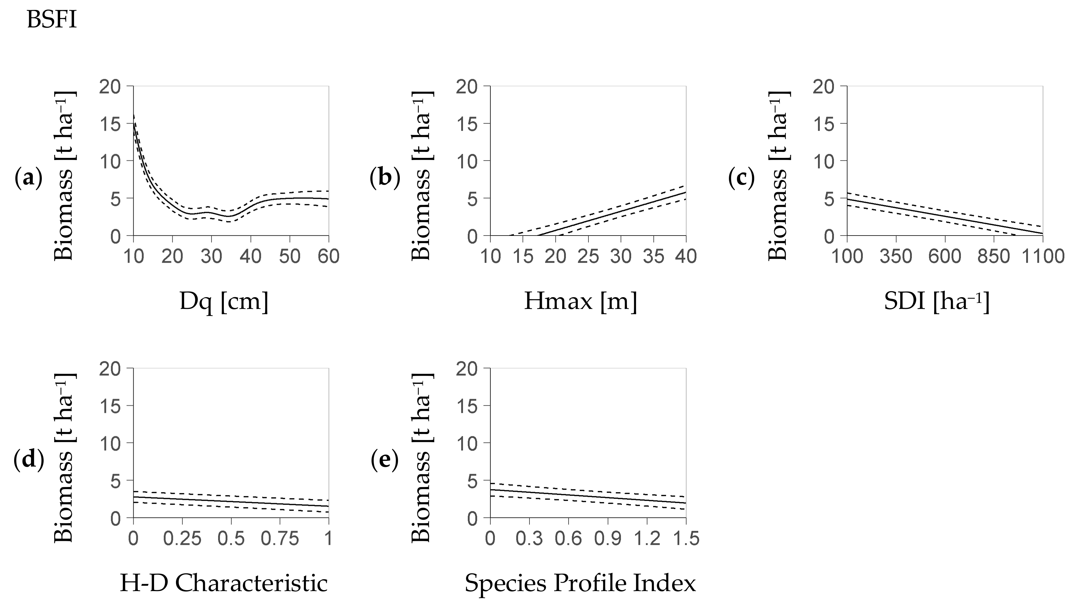
Figure 3.
Plausibility test of the theoretical probability distribution that provides the basis for the stochastic part of the model (Equation (8)); diagrams (a,b) are based on the NFI, i.e., German National Forest Inventory; (c,d) are based on the BSFI, i.e., Bavarian State Forest Inventory. That distribution of relative residuals (R in Equation (8), per-plot regeneration biomass to predicted regeneration biomass) is presented here from within a center range of the data (see Section 2.4) where the three main predictors of the deterministic model part (Figure 1), Dq, SDI, and Top Height, lie within their interquartile range each; both (a) (resp. (c)) and (b) (resp. (d)) compare the theoretical distribution to the empirical one; diagrams (a) and (c): probability density of the relative residual; the bars refer to the empirical density, and the line refers to the density obtained from a fitted gamma probability density function; diagrams (b) and (d): the QQ-plot of the quantile based on the fitted probability density function (Theoretical Quantile) over the quantile based on the measured data (Empirical Quantile); all shown within the 95% quantile of the relative residual ((a), (b) based on 1353 NFI plots, (c), (d) based on 1069 BSFI plots used for model calibration).


Figure 4.
Diagrams (a,b) show the parameters α and β of the stochastic model part (Equation (8)) based on the NFI (German National Forest Inventory), as represented by the trend line of shape α (diagram (a)) and rate β (diagram (b)) over the predicted regeneration biomass (Equations (9a) and (9b), parameterized equation shown above corresponding figure); the stochastic model part considers the scattering of the relative residuals of the deterministic part (Figure 1); diagram (c) is the result of the corresponding plausibility test of the stochastic model part with a QQ-Plot that compares 7784 quantiles Q of the modelled relative residual vs. the empirical one up to Q = 95% (relative residual is R in Equation (8), per-plot regeneration biomass to predicted regeneration biomass); diagrams (d–f) present the corresponding results based on the data of the BSFI (Bavarian State Forest Inventory, (d,e) based on 5881 plots used for model calibration; (f) based on 6073 points spared from calibration for evaluation).

Figure 5.
Diagrams (a,b): Mean of measured regeneration biomass over mean of predicted regeneration biomass per stratum obtained from the BSFI (Bavarian State Forest Inventory); (a) if strata have been formed based on the diameter class (Table 3); (b) if strata have both been formed based on diameter class and Forest Management Unit: the higher data spread on that scale level points to an as yet stochastic factor to be captured; in diagram (a), the numbers 4 to 60 denote diameter classes [cm] of 4 ± 4, 12 ± 3, 20 ± 5, 30 ± 5, 40 ± 5, 50 ± 5, and 55 to 80; in diagram (b), due to the sample size required per stratum the data focus on diameter classes 30, 40, and 50 (71% of all 11,954 BSFI plots); diagrams (c), (d) show the according result of the cumulative frequency (Cum. Freq.) of mean biomass; the cumulative frequency serves to indicate the quality of the modelled distribution characteristics (all based on 6073 inventory plots spared from model calibration for evaluation).

Table 1.
Value characteristics of the base data set from the German national forest inventory NFI (n = 7823) used to analyze the influence of the overstory on the biomass of the regeneration fraction. Columns q 2.5 and q 97.5 show the 2.5% and 97.5% quantile, respectively. Column n denotes the number of data records used to calculate that range, as well as the mean of the variable considered. Column Ori. (origin) indicates whether the data were native (N) or derived by own computation (D). Further abbreviations are Lr. (layer), BAF (basal area factor), ER (ecoregion), and EL (elevation).
| Lr. | Variable | Symbol | Basis | Level | Ori. | n | Mean | q 2.5 | q 97.5 | Unit |
|---|---|---|---|---|---|---|---|---|---|---|
| Overstory | tree diameter | Dt | -- | tree | N | 52,404 | 42 | 10 | 80 | cm |
| tree height | Ht | -- | tree | N | 52,404 | 28 | 11 | 40 | m | |
| tree number/ha | Nt | Dt BAF | tree | N | 52,404 | 76 | 7 | 520 | ha−1 | |
| Stand Density Idx. | SDI | Nt, Dt | plot | D | 7784 | 516 | 90 | 1 099 | -- | |
| Spec. Profile Idx. | SPI | Ht | plot | D | 7784 | 0.49 | 0 | 1.26 | -- | |
| H-D Characteristic | HD | Ht, Dt | plot | D | 7784 | 0.58 | 0.05 | 0.97 | -- | |
| Top height | Hmax | Ht | plot | D | 7784 | 30 | 13 | 42 | m | |
| Site Index | SI | ER, EL | plot | D | 7784 | 36.58 | 35.37 | 37.33 | m | |
| Quad. Mean Dia. | Dq | Nt, Dt | plot | D | 7784 | 36 | 11 | 67 | cm | |
| Regeneration | tree height | -- | -- | tree | N | 22,808 | 3.69 | 0 | 9 | m |
| tree diameter | -- | -- | tree | N | 22,808 | 0.7 | 0 | 5.5 | cm | |
| tree biomass | bc | -- | tree | N | 22,808 | 0.74 | 0 | 8.5 | kg | |
| tree number/ha | nc | -- | tree | N | 22,808 | 5253 | 0 | 31,831 | ha−1 | |
| biomass/ha | -- | bc, nc | plot | D | 7784 | 6.0 | 0 | 46 | t ha−1 | |
| tree number/ha | -- | nc | plot | D | 7784 | 15,392 | 0 | 98,218 | ha−1 |
Table 2.
Value characteristics of the base data set from the Bavarian State Forest inventory BSFI (n = 11,954) used to analyze the influence of the overstory on the biomass of the regeneration fraction. Columns q 2.5 and q 97.5 show the 2.5% and 97.5% quantile, respectively. Column n denotes the number of data records used to calculate that range, as well as the mean of the variable considered. Column Ori. (origin) indicates whether the data were native (N) or derived by own computation (D). Further abbreviations are Lr. (layer), BAF (basal area factor), ER (ecoregion), and EL (elevation).
| Lr. | Variable | Symbol | Basis | Level | Ori. | n | Mean | q 2.5 | q 97.5 | Unit |
|---|---|---|---|---|---|---|---|---|---|---|
| Overstory | tree diameter | Dt | -- | tree | N | 96,429 | 34 | 8.5 | 65 | cm |
| tree height | Ht | -- | tree | N | 96,429 | 25 | 9.3 | 37 | m | |
| tree number/ha | Nt | Dt BAF | tree | N | 96,429 | 73 | 15 | 404 | ha−1 | |
| Stand Density Idx. | SDI | Nt, Dt | plot | D | 11,954 | 519 | 74 | 1080 | -- | |
| Spec. Profile Idx. | SPI | Ht | plot | D | 11,954 | 0.6 | 0 | 1.4 | -- | |
| H-D Characteristic | HD | Ht, Dt | plot | D | 11,954 | 0.54 | 0.03 | 0.95 | -- | |
| Top height | Hmax | Ht | plot | D | 11,954 | 29 | 10 | 40 | m | |
| Site Index | SI | ER, EL | plot | D | 11,954 | 35.4 | 36.25 | 37.33 | m | |
| Quad. Mean Dia. | Dq | Nt, Dt | plot | D | 11,954 | 32 | 9.7 | 59 | cm | |
| Regeneration | tree height | -- | -- | tree | N | 42,342 | 2.18 | 0.2 | 9.2 | m |
| tree diameter | -- | -- | tree | N | 42,342 | 1.4 | 0 | 6.5 | cm | |
| tree biomass | bc | -- | tree | N | 42,342 | 1.4 | 0 | 12 | kg | |
| tree number/ha | nc | -- | tree | N | 42,342 | 2503 | 321 | 16,040 | ha−1 | |
| biomass/ha | -- | bc, nc | plot | D | 11,954 | 4.3 | 0 | 30 | t ha−1 | |
| tree number/ha | -- | nc | plot | D | 11,954 | 7667 | 0 | 47,705 | ha−1 |
Table 3.
Classification levels of the average diameter used for stratification with pct of plots in the BSFI (Bavarian State Forest Inventory) data (see Section 2.1.2).
Table 3.
Classification levels of the average diameter used for stratification with pct of plots in the BSFI (Bavarian State Forest Inventory) data (see Section 2.1.2).
| Class | Diameter [cm] 1 | Pct of Plots |
|---|---|---|
| 4 | 0 to 8 | 3 |
| 12 | 8 to 15 | 6 |
| 20 | 15 to 25 | 15 |
| 30 | 25 to 35 | 28 |
| 40 | 35 to 45 | 28 |
| 50 | 45 to 55 | 15 |
| 60 | 55 and more | 5 |
1 Lower limit excluded.
Table 4.
Coefficients of the regeneration biomass model based on the NFI (German National Forest Inventory, Equations (4a) and (5)). The variables are denoted as in Equations (4a) and (5), i.e., SDI (Stand Density Index), SPI (Species Profile Index), SI (Site Index), Hmax (maximum height), HD (Height Diameter Characteristic), Dq (Quadratic Mean Diameter); β1 to β5 are corresponding fixed effect coefficients; s(Dq) is a univariate penalized cubic regression spline [31] over Dq (Figure 1a); b is the NFI cluster specific random effect, and s1 is its standard deviation; ε represents the i.i.d. errors and s2 represents their standard deviation.
| Intercept | Fixed Effect of | Random Effect | |||||||
|---|---|---|---|---|---|---|---|---|---|
| SDI | SPI | SI | Hmax | HD | s(Dq) | bi | εij | ||
| Symbol 1 | β0 | β1 | β2 | β3 | β4 | β5 | -- | s1 | s2 |
| Value | 74,344 | −6.87 | −1498 | −1304 | 304 | −2927 | -- | 5536 | 11,750 |
| SE | 143 | 0.60 | 380 | 265 | 32 | 692 | -- | ||
| p-value | <0.0001 | <0.0001 | <0.0001 | <0.0001 | <0.0001 | <0.0001 | <0.0001 | ||
1 In Equation (4a).
Table 5.
Coefficients of the regeneration biomass model based on the BSFI (Bavarian State Forest inventory, Equations (4b) and (6)). Site Index (SI) was not significant as a predictor and removed from Equation (4b) (see Section 2.4); the variables are denoted as in Equations (4b) and (6), i.e., SDI (Stand Density Index), SPI (Species Profile Index), Hmax (maximum height), HD (Height Diameter Characteristic), Dq (Quadratic Mean Diameter); β1 to β5 are corresponding fixed effect coefficients; s(Dq) is a univariate penalized cubic regression spline [31] over Dq (Figure 2a); bi is the random effect specific for the forest management unit, and s3 is its standard deviation; bij is the stand specific random effect, and s4 is its standard deviation; εij represents the i.i.d errors and s5 represents their standard deviations.
| Intercept | Fixed Effect of | Random Effect | ||||||||
|---|---|---|---|---|---|---|---|---|---|---|
| SDI | SPI | SI | Hmax | HD | s(Dq) | bi | bij | εijk | ||
| Symbol 1 | β0 | β1 | β2 | -- | β4 | β5 | -- | s3 | s4 | s5 |
| Value | 40,074 | −4.59 | −1194 | -- | 255 | −4610 | -- | 1150 | 3667 | 7684 |
| SE | 251 | 0.48 | 289 | -- | 26 | 571 | -- | |||
| p-value | <0.0001 | <0.0001 | <0.0001 | -- | <0.0001 | <0.0001 | <0.0001 | |||
1 In Equation (4b).
Table 6.
The increase of the AIC related to each predictor when it was removed as the only one from Equation (4a) and the nested model of Equation (4b) with minimum AIC (see Section 2.4). Abbreviations are NFI (German National Forest Inventory) and BSFI (Bavarian State Forest Inventory).
Table 6.
The increase of the AIC related to each predictor when it was removed as the only one from Equation (4a) and the nested model of Equation (4b) with minimum AIC (see Section 2.4). Abbreviations are NFI (German National Forest Inventory) and BSFI (Bavarian State Forest Inventory).
| Model | Increase in AIC Related to Predictor | |||||
|---|---|---|---|---|---|---|
| SDI | SPI | SI | Hmax | HD | s(Dq) | |
| NFI (Equation (4a)) | 96 | 14 | 10 | 127 | 10 | 229 |
| BSFI (Equation (4b)) | 388 | 67 | -- | 406 | 253 | 2682 |
© 2018 by the authors. Licensee MDPI, Basel, Switzerland. This article is an open access article distributed under the terms and conditions of the Creative Commons Attribution (CC BY) license (http://creativecommons.org/licenses/by/4.0/).
Share and Cite
MDPI and ACS Style
Poschenrieder, W.; Biber, P.; Pretzsch, H. An Inventory-Based Regeneration Biomass Model to Initialize Landscape Scale Simulation Scenarios. Forests 2018, 9, 212. https://doi.org/10.3390/f9040212
AMA Style
Poschenrieder W, Biber P, Pretzsch H. An Inventory-Based Regeneration Biomass Model to Initialize Landscape Scale Simulation Scenarios. Forests. 2018; 9(4):212. https://doi.org/10.3390/f9040212
Chicago/Turabian StylePoschenrieder, Werner, Peter Biber, and Hans Pretzsch. 2018. "An Inventory-Based Regeneration Biomass Model to Initialize Landscape Scale Simulation Scenarios" Forests 9, no. 4: 212. https://doi.org/10.3390/f9040212
Note that from the first issue of 2016, this journal uses article numbers instead of page numbers. See further details here.