Article

Stock Volume Dependency of Forest Drought Responses in Yunnan, China

1
Key Laboratory of Environmental Change and Natural Disaster of Ministry of Education, Academy of Disaster Reduction and Emergency Management, Faculty of Geographical Science, Beijing Normal University, Beijing 100875, China
2
State Key Laboratory of Earth Surface Processes and Resource Ecology, Beijing Normal University, Beijing 100875, China
3
School of Earth and Environmental Sciences, Queens College of the City University of New York, New York, NY 11367, USA
4
Earth and Environmental Sciences Department, the Graduate Center of the City University of New York, New York, NY 10016, USA
5
State Key Laboratory of Remote Sensing Science, Jointly Sponsored by Beijing Normal University and Institute of Remote Sensing and Digital Earth of Chinese Academy of Sciences, Beijing 100875, China
*
Author to whom correspondence should be addressed.
Forests 2018, 9(4), 209; https://doi.org/10.3390/f9040209
Submission received: 20 February 2018 / Revised: 5 April 2018 / Accepted: 13 April 2018 / Published: 16 April 2018
(This article belongs to the Special Issue Remotely Sensing of Drought-Induced Forest Change and Recovery)

Abstract

:
Revealing forest drought response characteristics and the potential impact factors is quite an important scientific issue against the background of global climate change, which is the foundation to reliably evaluate and predict the effects of future drought. Due to the high spatial heterogeneity of forest properties such as biomass, forest age, and height, and the distinct differences in drought stress in terms of frequency, intensity, and duration, current studies still contain many uncertainties. In this research, we used the forests in Yunnan Province in Southwest China as an example and aimed to reveal the potential impacts of forest properties (i.e., stock volume) on drought response characteristics. Specifically, we divided the forest into five groups of stock volume density values and then analyzed their drought response differences. To depict forest response to drought intensity, the standardized precipitation evapotranspiration index (SPEI) was chosen as the explanatory variable, and the change in remote sensing-based enhanced vegetation index (deficit of MODIS-EVI, dEVI) was chosen as the response variable of drought stress. Given that the SPEI has different time scales, we first analyzed the statistical dependency of SPEIs with different time scales (1 to 36 months) to the response variable (i.e., dEVI). The optimal time scale of SPEI (SPEIopt) to interpret the maximum variation of dEVI (R-square) was then chosen to build the ultimate statistical models for the five groups of stock volume density. The main findings were as follows: (1) the impacts of drought showed hysteresis and cumulative effects, and the length of the hysteresis increased with stock volume densities; (2) forests with high stock volume densities required more soil water and were therefore more sensitive to the changes in water deficit; (3) compared with the optimal time scale of SPEI (SPEIopt), the SPEI with the commonly used time scale (e.g., 1, 6, and 12 months) could not well reflect the impacts of drought on forests and the simulation error of dEVI increased with stock volume densities; and (4) forests with higher stock volume densities were likely to experience a greater risk of degradation following higher atmospheric concentrations of greenhouse gases (Representative Concentration Pathway (RCP) 8.5). As a result, both the time scale of the meteorological drought index and the spatial difference in forest stock volumes should be considered when evaluating forest drought responses at regional and global scales.

Graphical Abstract

1. Introduction

Forest ecosystems offer products (e.g., food, timber) and services (e.g., soil, water conservation, climate moderation) [1,2,3], and are therefore crucial to the survival and sustainable development of societies. As global temperatures rise and patterns of precipitation change [4,5], forest ecosystems are experiencing an increase in gradual risk [6]. In recent years, drought has been more frequent, more severe, and longer [7,8]. It has affected forest ecosystems to varying degrees [6,9,10], and has threatened forest health and affected ecosystem services, so it is important to manage forests efficiently through informed decision-making that reliably evaluates and predicts the effects of drought on forest growth [11].
A tree response to drought includes a series of adjustments and corresponding characteristic responses. In the early stages of drought, stomata are kept open as far as possible, and regular growth is maintained through continuous assimilation of CO2 [12,13]; as the stress intensifies, stomata are closed to reduce water loss. Meanwhile, root growth is accelerated to increase the uptake of soil moisture [13,14]. When the intensity of drought stress exceeds the tree’s ability to adapt and resist the stress, other physiological responses set in, manifesting in the yellowing of leaves and leaf shedding [14,15], and the tree eventually dies from xylem embolism, carbon starvation, or both [16,17,18]. The question of how to use methods such as remote sensing, meteorological drought index, ground surveys, and various other ways to recognize the onset of drought and assess its impact in different intensities of drought is one of the key areas of research today.
By exploiting the growing abundance of information from both remote sensing and ground surveys, researchers have made commendable progress in monitoring and evaluating drought. Nevertheless, some critical conclusions remain controversial. In terms of causes, the effects of drought on forest can be seen from two aspects. One is the intensity of external stress (e.g., drought intensity and duration), and the other is the different attributes of the forest itself (e.g., biomass, age, and height), for instance, the responses of forests to a given intensity of drought, which vary widely depending on the age and the height of trees. From the view of tree height, some researchers have suggested that tall trees require more moisture to support and maintain their regular growth (e.g., the stem, leaves, and the xylem conduit system) [19], and are therefore more vulnerable to drought. Other researchers have considered such trees to be able to synthesize more carbohydrates and thereby make up for carbon starvation as they are able to capture more sunlight and have more effective photosynthesis [20,21]. From the perspective of tree age, some researchers have found that the risk of xylem embolism is greater in older trees as they are less efficient in taking up soil moisture and have fewer fine roots [22,23], whereas other researchers maintain that older trees are better at resisting drought as their deeper root systems can access phreatic water from greater depths [24,25].
Aside from these differences in forest attributes, some uncertainties in expressing the effects of external drought will be added in different ways. The response of trees to moisture is related not only to the current water balance, but also to past precipitation and temperature, which shows a clear time lag [26] and legacy effects [27]. Some researchers have found a time lag for the response of forests to drought, the effect of the continuous cumulative water deficit, or the surplus condition on forest growth being greater [26,27]. Based on the correlations between meteorological data, the annual tree rings, and remote sensing vegetation index, Wu et al. reported that forests (trees and shrubs) took more than two years to respond to drought in the temperate zone of the northern hemisphere [27]. Thus, if the differences in response characteristics (e.g., the length of hysteresis) of forests with different stock volume densities are fully taken into account, the response of forests to drought can be evaluated more reliably [10,28,29].
The present research considered two types of indexes—meteorological drought indexes (e.g., the Palmer drought severity index (PDSI), the standardized precipitation index (SPI), and the standardized precipitation evapotranspiration index (SPEI)) [30,31,32], calculated on the basis of such meteorological variables as temperature and precipitation; and vegetation indexes (e.g., the normalized difference vegetation index (NDVI) and the enhanced vegetation index (EVI) [33]) based on remote sensing—in evaluating the effect of drought. Meteorological drought indexes are simpler to calculate [34] and can predict climate change using a climate model [35,36] but ignore spatial differences in vegetation and the differences in the response characteristics of vegetation with different attributes to drought and thus reflect meteorological drought rather than agricultural or hydrological drought [34,37]. Vegetation indexes based on remote sensing not only directly reflect changes in the growth of vegetation, but also have a high temporal and spatial resolution, and therefore can reflect the differences in the response of vegetation with different attributes to drought. This is why vegetation indexes are always used in characterizing the response of forests to drought on regional and global scales [33,38].
Thus, to reveal the potential impacts of forest stock volume on drought response characteristics, forests in Yunnan Province of China were chosen as an example for the present research, and an SPEI with different time scales that could reflect drought characteristics was taken as the explanatory variable; the variation (dEVI, or the deficit of EVI) in MODIS-EVI was used as the response variable of forests with different stock volume densities. Thus, it was possible to assess and predict the effects of drought on forests more reliably.

2. Materials and Methods
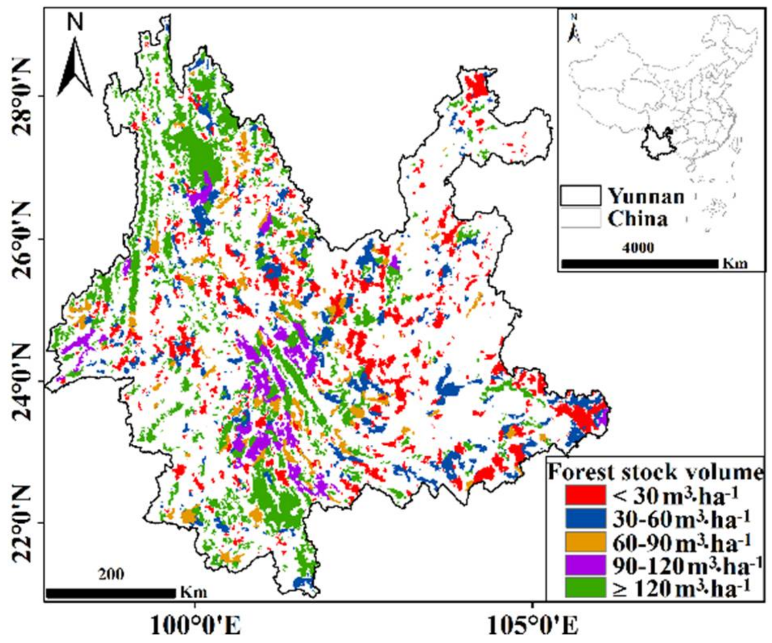
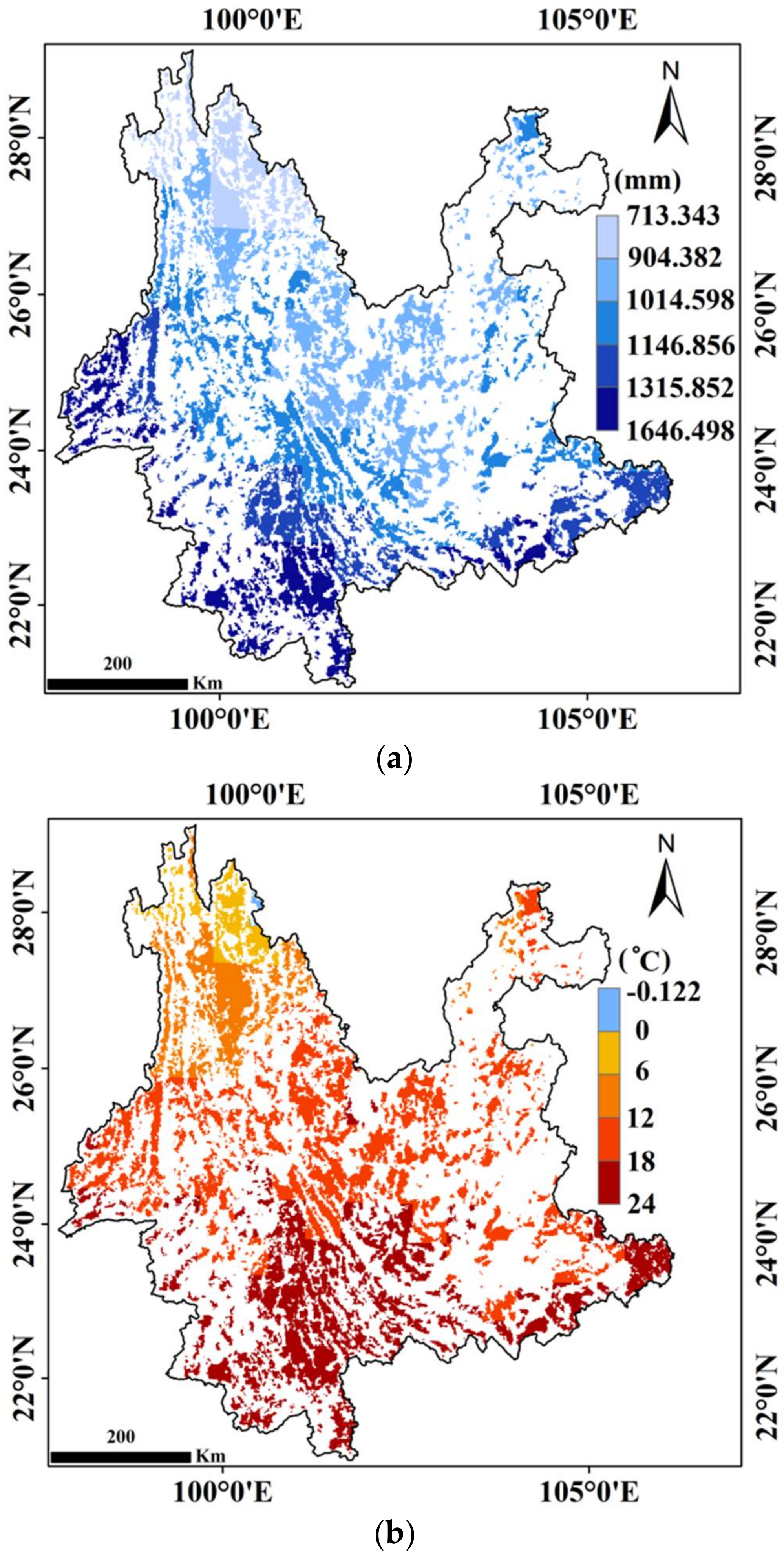
2.1. Research Area

Yunnan Province (21.13°–29.25° N, 97.51°–106.18° E) is located in southwestern China (Figure 1), and primarily has a subtropical monsoon, plateau monsoon, and tropical rainy climate. The precipitation and temperature of Yunnan Province show a regular change where both decrease gradually from south to north (Figure 2a,b); this is related to the water resource and the latitude location. Based on the data mentioned above, the research found that Yunnan Province, with a mean annual precipitation (MAP) of 1098.6 mm and a mean annual temperature (MAT) of 15.7 °C, is warm and humid in general. In addition, the precipitation and temperature are concentrated in summer (June–August) [10], and therefore it is a typical high-coverage region in China, where the forest cover is greater than 50.0% [39]; forests with various stock volume densities are widely distributed (Figure 1) [40], and the best status of forests grow mainly in summer (especially in July) [10]. From 2001 to 2014, large areas of Yunnan suffered many drought events (2005–2006, 2009–2014) with varying intensities and duration, which significantly affected the forest ecosystem [10,41,42]. Typical drought events in Yunnan include the mild drought of 2005 and the persistent drought in winter of 2009 to spring of 2010 [10,41]. Yunnan Province is currently a focus study region for exploring how the forest responds to drought as it has a high forest cover rate and has suffered several drought events [43,44], especially from 2001–2014. Due to all of these reasons, Yunnan Province was selected as the study region.

2.2. Materials

2.2.1. Distribution Map of Forest Stock Volume

Forests in China show a highly significant and linear relationship between biomass density (Mg·ha−1) and stock volume density (m3·ha−1), with a correlation coefficient of 0.98 at the level of provincial forests [47]. The forest stock volume density increases in a nonlinear manner with the increase in age and height [48,49]. Therefore, the grade map of forest (arbor forest) stock volume density was taken as an indicator in the present research (Figure 1) [40]. The map was obtained from the Seventh National Forest Resources Inventory, which was carried out over five years (2004–2008) based on the provincial administration and provided by each province [50] and is the foremost data set of forest resources. A total of 0.415 million permanent sample plots were chosen to acquire 0.16 billion groups of inventory data, where the data form the basis of the map [50]. All the forests in the province were divided into five groups on the map as follows: less than 30 m³·ha−1 (<30), which accounted for 25.24% of the total forested area; 30–60 m3·ha−1 (18.15%), 60–90 m³·ha−1 (9.89%); 90–120 m3·ha−1 (8.64%); and greater than or equal to 120 m3·ha−1 (≥120) (38.08%) [40]. To relate the distribution to the remote sensing vegetation index, the map was first digitized and then converted to one with a spatial resolution of 1 km by spatial adjustment and resampling using ArcGIS (ver. 10.2) (Esri, Environmental Systems Research Institute, New York, NY, USA).

2.2.2. MODIS-Enhanced Vegetation Index

Compared with the NDVI, the EVI is more sensitive to information from high-coverage regions and is therefore less likely to be saturated [33,51]. As the research region (Yunnan Province, southwest China) of this study is a typical high-coverage region in China (where forest cover is greater than 50%) [39], EVI is more suitable than NDVI to characterize the forest growth status in the present research. In addition, the moderate imaging spectroradiometer (MODIS) not only has the time continuity of data, but its spatial resolution can also meet the needs of research in the medium scale [33,44]. Thus, the MOD13A1-EVI product from the land processes distributed active archive center, which is provided every 16 days at a resolution of 500 m, was chosen for the present research [52]. The monthly EVI was obtained as a composite of many EVI diagrams for each month and expressed as the maximum value composite (MVC) [53]. To match the forest data, the EVI was resampled to 1 km using ArcGIS (ver. 10.2) (Esri, Environmental Systems Research Institute, New York, NY, USA). As July is the most conducive for forest growth, and the trees in this month are most sensitive to moisture status [10,28], only the EVI for July in each year was selected to represent the status of forest growth in that year. Furthermore, the start time of the MOD13A1-EVI was 2001 [52], and the deadline of SPEIbase ver. 2.4 (the Climatic Research Unit (CRU)) was 2014 [46]. In addition, Yunnan had several dry years (2005–2006, 2009–2014) and wet years (2001–2004, 2007–2008) during 2001 to 2014 [10,41,42], so the 2001–2014 databases were selected in this research. From the spatial distribution of the mean annual EVI during 2001–2014, a large spatial difference in forest growth status (Figure 3a) was found, which could be due to the distribution of different forest stock volume densities as many researchers have shown a positive relationship between forest stock volume density and EVI [54]. The variation in forest growth status shown by the annual standard deviation of EVI (Figure 3b) could be driven by external stresses such as drought.
To reflect the change in EVI, which is directly related to environmental stress (e.g., drought), and to reduce the complicated impacts caused by both biotic and abiotic factors on the EVI itself, we constructed the deficit index of EVI (dEVI) at the grid scale: the maximum EVI (EVImax) was calculated at each spatial grid over the study period (2001–2014), and the grid with EVImax was considered to be the ideal condition without any drought stress; therefore, the corresponding value was taken to be the reference of EVI. Finally, the difference between EVIi and EVImax was calculated for each year (Equation (1)). As the dEVIi reflected the relative reduction in EVI caused by drought in the ith year, it was more directly related to meteorological drought indexes that reflect the relative water deficit or surplus such as the SPEI.
d E V I i = E V I i E V I max E V I max × 100 %
where EVIi is the EVI of July in the ith year, and EVImax is the maximum EVI of July during the 14-year period (2001–2014).

2.2.3. Meteorological Drought Index

There are several extensively used climate drought indices such as SPEI, PDSI, and SPI, etc. [30,31,32], each with its own advantage. However, SPEI incorporates the advantages of PDSI that are sensitive to the evaporative demand, and that of SPI with multiple time scales [32,55,56], so the SPEI reflected the cumulative effects of water deficit and surplus over multiple time scales in the research. In calculating the water balance, SPEI was calculated as follows [32,55]: (1) potential evapotranspiration (PET) was obtained by the Thornthwaite and the Penman–Monteith models; (2) different time scales of the cumulative effects of water deficit and surplus were calculated; (3) the three-parameter log-logistic probability density function was adopted to fit the established cumulative series; and (4) the cumulative series was converted by the standard normal distribution.
The monthly SPEI data for the period 2001–2014 were derived from SPEIbase ver. 2.4, which has a spatial resolution of 0.5° [46]. The data set comprised monthly precipitation and potential evapotranspiration values obtained from CRU of the University of East Anglia, UK, and potential evapotranspiration in SPEIbase was calculated using the FAO-56 Penman–Monteith method. To match the other data, the SPEI data sets were resampled to the resolution of 1 km using ArcGIS (ver. 10.2) (Esri, Environmental Systems Research Institute, New York, NY, USA).
To estimate the potential impact of the changes of water deficit on forest growth, the SPEI was calculated for a range of scenarios (representing different atmospheric concentrations of greenhouse gases (GHGs)), based on the temperature and precipitation data estimated by a model, namely, CMIP5 (Coupled Model Inter-comparison Project Phase 5). The estimates were grouped into four submodels: GFDL-ESM2M [57], IPSL-CM5A-LR [58], MIROC-ESM-CHEM [59], and NorESM1-M [60], at two extremes of the concentrations of GHGs, representative concentration pathway (RCP) 2.6 and RCP 8.5, which cover the daily average temperature and precipitation data at a resolution of 0.5° for the period 1950–2099 (the present research considered only the 2015–2099 subset). Given the greater uncertainty in estimating values from a single set, the average of the four climate models was used. Finally, the monthly SPEI (SPEIfuture) at different time scales was calculated based on the monthly average temperature and precipitation under the RCP 2.6 and RCP 8.5 scenarios. Two competing methods of estimating PET, namely, the Thornthwaite and Penman–Monteith methods, because their corresponding results (SPEI) were similar in a humid region such as Yunnan Province [61], and the Thornthwaite method requires only the monthly average temperature and precipitation data to calculate the PET, so the Thornthwaite method was used in the present research and it’s calculation procedure was derived from DIGITAL.CSIC [62]. To make them consistent with other data, the original values of SPEIfuture (at a resolution of 0.5°) were resampled to the resolution of 1 km.

2.3. Methods

2.3.1. Optimal Time Scale for SPEI

Forest growth is affected by precipitation and evapotranspiration not only in the current month, but also in the preceding months. The effect of water balance on forest growth clearly shows hysteresis [26], and its length depends on the vegetation type, which shows distinct spatial patterns. Some researchers have found that it takes many months before the effects of moisture are apparent [10,26], and the length of such hysteresis can be a year [28,29] or even 2–3 years [63]. Due to the hysteretic effects of moisture, the SPEI was not calculated for a given time scale initially; instead, it was calculated for multiple time scales.
By comparing the association strength between the SPEI at multiple time scales and dEVI, the research selected the optimal time scale for SPEI. Taking into account the differences in hysteresis (as related to water balance) between the different stock volume densities, the impact of drought could be assessed more accurately. In determining the optimal time scale for SPEI, linear regression models (SPEI-dEVI) between the SPEI on 1–36 month time scales and the dEVI of forests with five groups of stock volume density were constructed, and 180 regression models were generated in this exercise. Next, according to the significance (at the 0.01 level) and the R2 of the linear regression models, the optimal time scale and the corresponding SPEI (SPEIopt) were determined. To ensure the selected time scale and the corresponding SPEI were truly representative and robust, the average values of R2 in these regression models, between the SPEI on adjacent time scales and dEVI, were used as references; in other words, sliding windows of three months and five months were used to confirm the average value of R2 on adjacent time scales. To reduce the interference from miscellaneous data, the average values of SPEI and dEVI in every grade of drought (eight grades) [64] (Table 1), were used as the base data for the linear regression models.

2.3.2. Response to Drought as Affected by Different Forest Stock Volumes

For the forests in each stock volume density group, that is, from less than 30 m3·ha−1 to greater than or equal to 120 m3·ha−1 in increments of 30 m3·ha−1, and on the basis of SPEIopt, a linear regression model was established between SPEIopt and the corresponding dEVI (SPEIopt-dEVI). Next, to assess the sensitivity of stock volume to dEVI following changes in the level of moisture, the differences in the coefficients of determination (R2) and the regression coefficients from the models between different forest stock volume densities were compared. At the same time, the dEVI in the future (dEVIfuture) was first calculated using the SPEIopt-dEVI model and SPEIfuture data; the patterns of temporal changes and the relative risk from climate change to forests between five groups of stock volume density were compared and ascertained, respectively. Due to the limitations of forest stock volume data, the extent of forest cover and the total area under forests were assumed to remain the same in the future and in only one of the five groups of stock volume density.
Additionally, to evaluate the magnitude of the potential error from the SPEI (SPEIfix) that was assigned artificially to a fixed time scale and because any difference due to the stock volume (the stock-volume-independent time scale for the SPEI) was ignored, the research compared the differences in the simulated dEVI between SPEIfix and the SPEIopt that were related to the stock volume density (the stock-volume-dependent time scale for the SPEI). Finally, the common SPEIfix of three fixed time scales, namely, 1 month (SPEI1), 6 months (SPEI6), and 12 months (SPEI12), was adopted in the research. All the statistical methods and statistical mapping were completed using Matlab (R2012b) (MathWorks, Natick, MA, USA).

3. Results

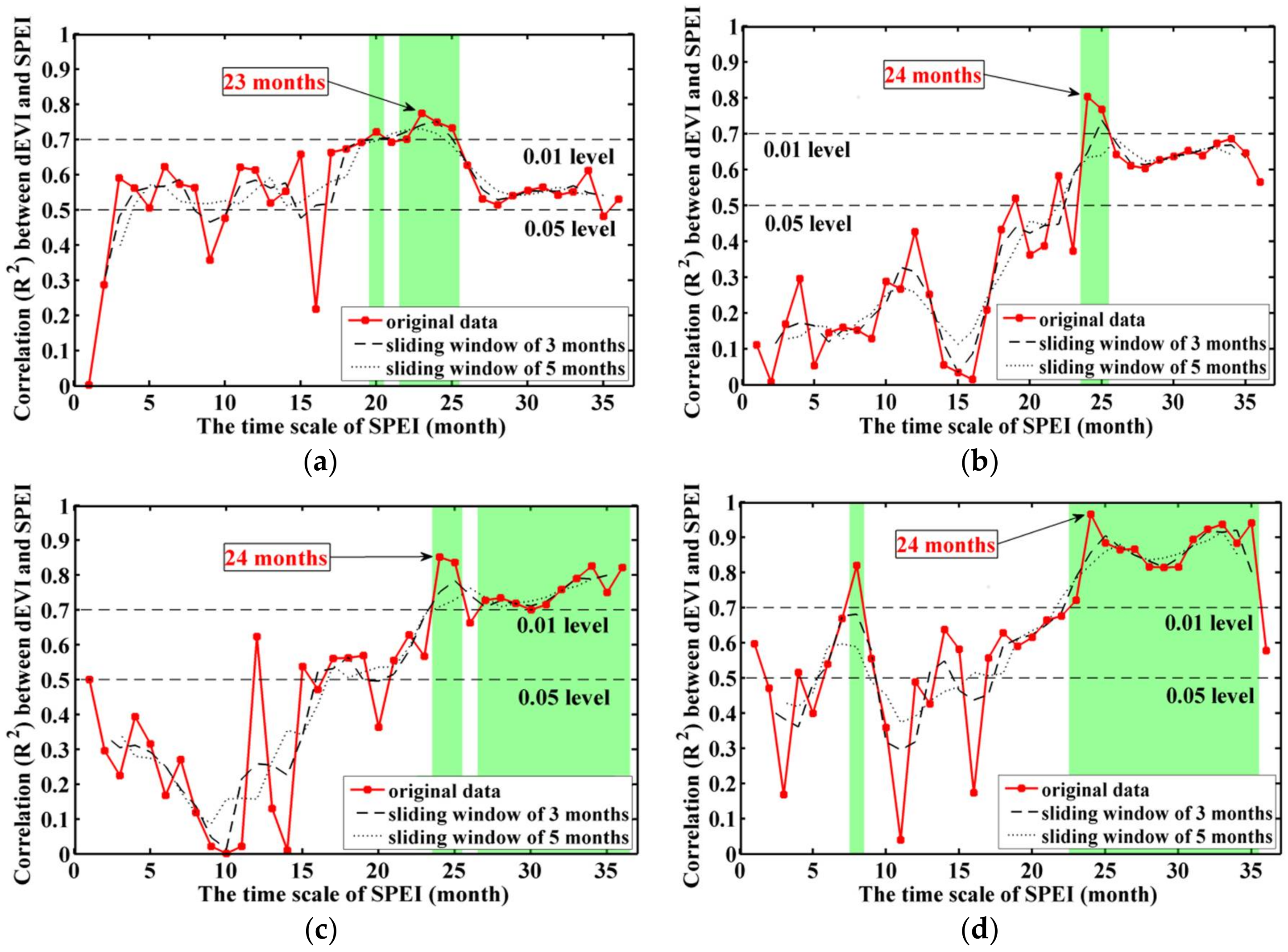
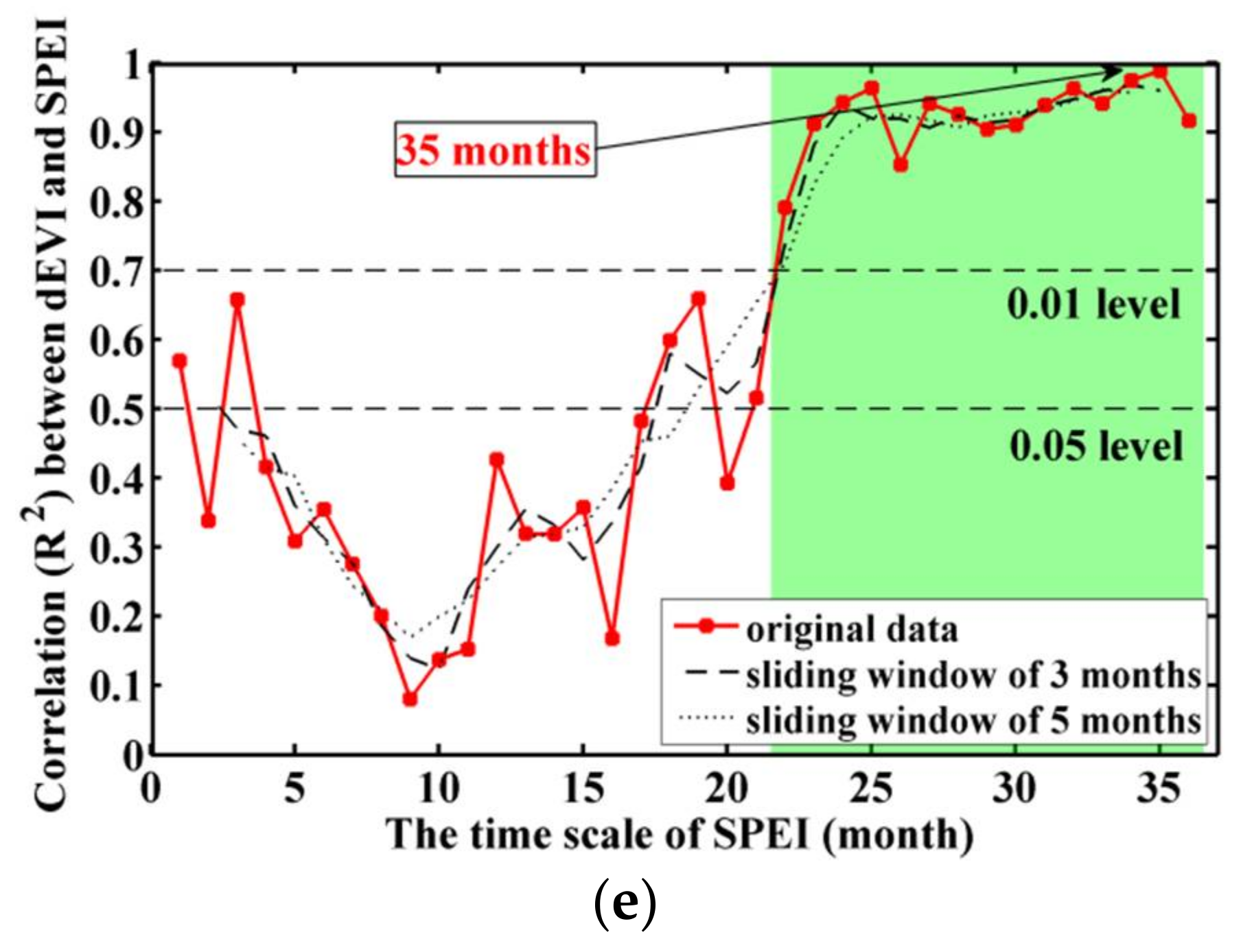
3.1. Stock-Volume-Dependent Time Scales of SPEI

A clear relationship was seen between the SPEI (which reflected meteorological drought) and the dEVI (which reflected physiological drought), although the strength of that relationship varied markedly, depending on the time scale of SPEI and on the forest stock volume density (Figure 4). Overall, the association strength (R2) between SPEI and dEVI varied greatly with the time scale of the SPEI. At the level of 0.01, the relationship between dEVI and the SPEI for most of the time scales was statistically non-significant, which indicated that a suitable time scale was required for SPEI when evaluating or predicting the effect of drought.
The difference in the demand for and the supply of water between forests with different stock volume densities affects the optimal time scale of the meteorological drought index. For forests with low stock volume densities, the most suitable time scale was 23–24 months: for scales shorter or longer than that, the association strength between SPEI and dEVI decreased markedly (Figure 4a,b). However, for forests with high stock volume densities, the most suitable time scale was 24 months in most cases: the R2 (association strength) did not decrease at time scales longer than 24 months (Figure 4c–e).
Comparing the R2max of the linear regression models that considered the relationship between the dEVI and the SPEI at different time scales, and with reference to the average R2 values for the sliding windows of three and five months on adjacent time scales as well as the significance level, the optimal time scale of SPEI for each stock volume density was as follows: 23 months for stock volume densities less than 30 m3·ha−1; 24 months for each of the next three groups; and 35 months for stock volume densities greater than or equal to 120 m3·ha−1 (Figure 4a–e). Overall, the optimal time scale increased as the stock volume density increased. This trend means that longer times of hysteresis and the cumulative effects of water balance need to be considered when evaluating the effects of drought on forests on the basis of a meteorological drought index.

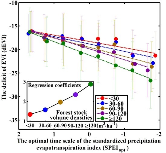
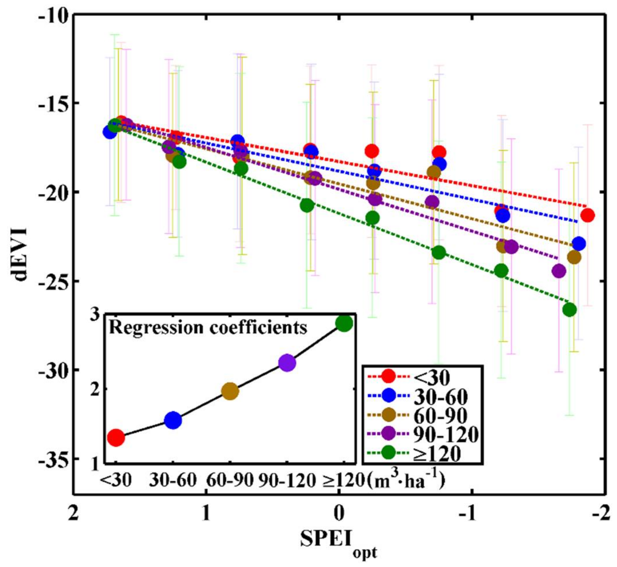
3.2. Differences in Sensitivity to Drought between Different Forest Stock Volumes

Based on the analysis of the linear regression between the SPEI at 1–36 month time scales and the dEVI of forests with different stock volume densities, the optimal time scale of SPEI (SPEIopt) was determined, and the optimal model that best simulated the response of the vegetation to water, as judged on the basis of SPEIopt, was determined (Table 2). Models for the optimal time scales showed the maximum variance interpretation rate (R2) and therefore reflected to the fullest extent the relationship between meteorological drought and physiological drought. Irrespective of the forest stock volume density, the dEVI reflecting forest growth status decreased gradually as the intensity of the drought increased. In addition, it was found that the R2 of a model increased gradually as the stock volume density increased (Table 2). Furthermore, the sensitivity of dEVI to changes in the moisture status also increased as the stock volume density increased; that is, a unit change in the moisture content caused a greater reduction in the dEVI for forests with higher stock volume densities (Figure 5). Thus, the relationship between drought stress intensity and its effects on forests was stronger, and forests were more sensitive to changes in soil moisture when the forests had high stock volume densities—their resistance to such changes was weaker during times of drought.

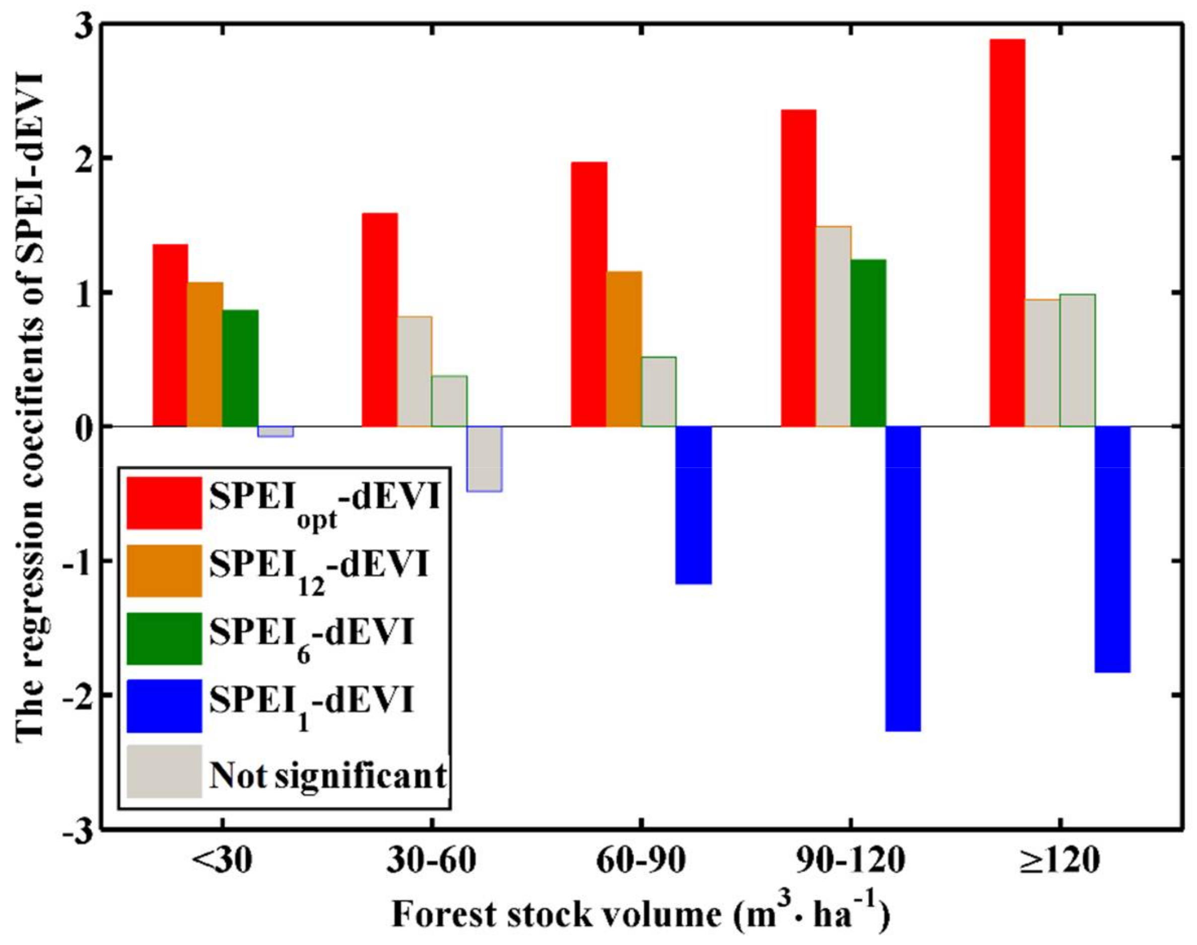
3.3. Error Caused by Stock-Volume-Independent Time Scale of SPEI

To measure in quantitative terms the potential effect of stock-volume-independent time scale on the simulated error in dEVI, the differences in the dEVI from simulations and the optimal model that considered the forest stock volume (a stock-volume-dependent time scale) were compared and analyzed. Three common time scales (1 month, 6 months, and 12 months) were selected as the fixed time scales for the SPEI.
If the differences in terms of stock volume were ignored, and if the SPEI that was assigned artificially to a fixed time scale was used for simulating the response of vegetation to drought, the following problems arose. First, the relationship between changes in the SPEI and those in the EVI was represented incorrectly, as evident from the negative correlation between the SPEI at a 1-month time scale and dEVI (SPEI1-dEVI in Figure 6), as precipitation in the current month only had a limited effect on forest growth [29]. Excess precipitation is always accompanied by a decrease in photosynthetically active radiation and by lower temperatures, so forest growth is affected adversely [26]. Second, the relationship between SPEI and dEVI was revealed correctly, but the significance level and the statistical significance of the model were underestimated (grey icon in Figure 6). Third, despite overcoming the above two shortcomings, the model parameter that reflected changes in the dEVI, which changes with the drought stress intensity, was potentially underestimated, and therefore forest growth sensitivity to drought as a result of climate change (Figure 6).

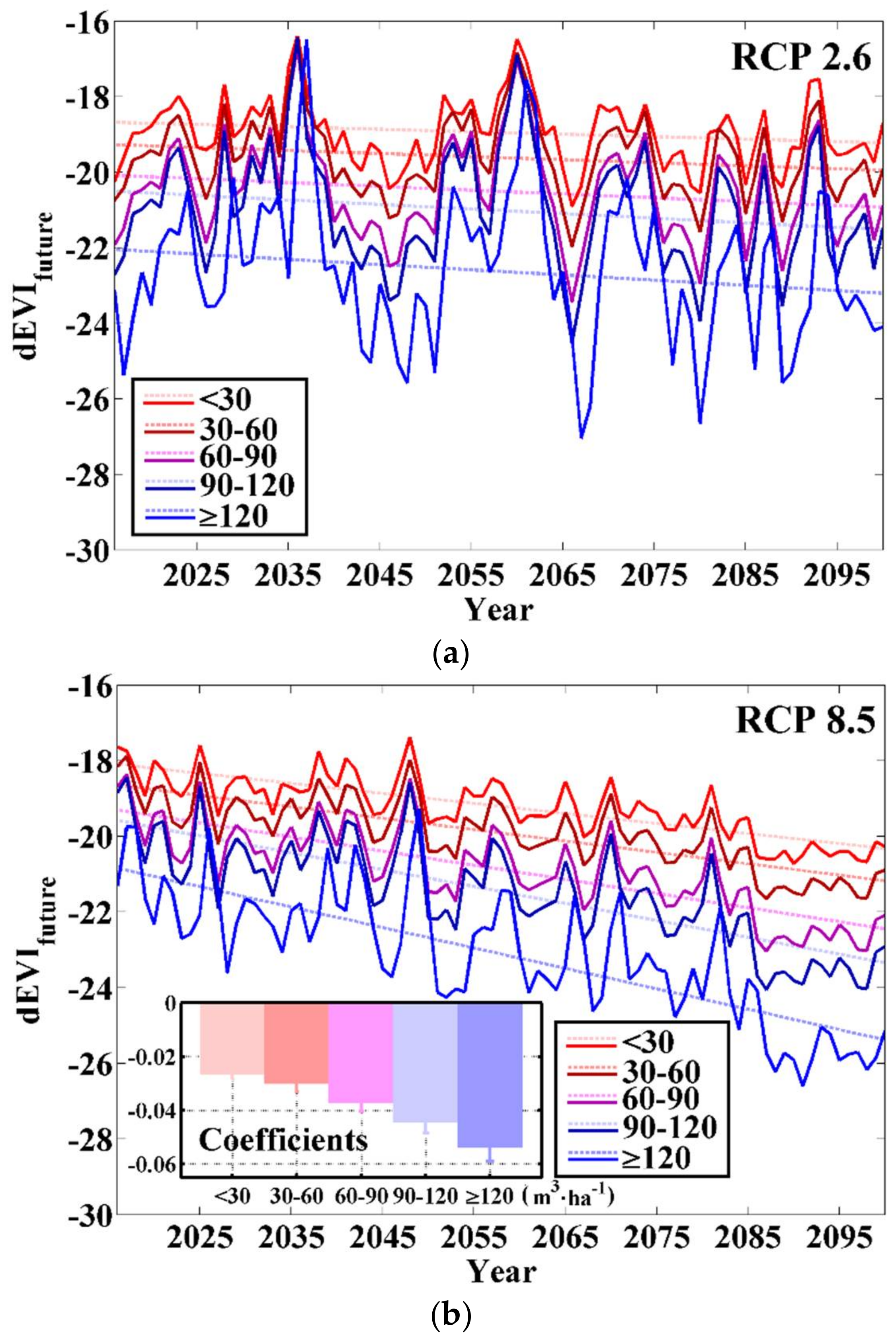
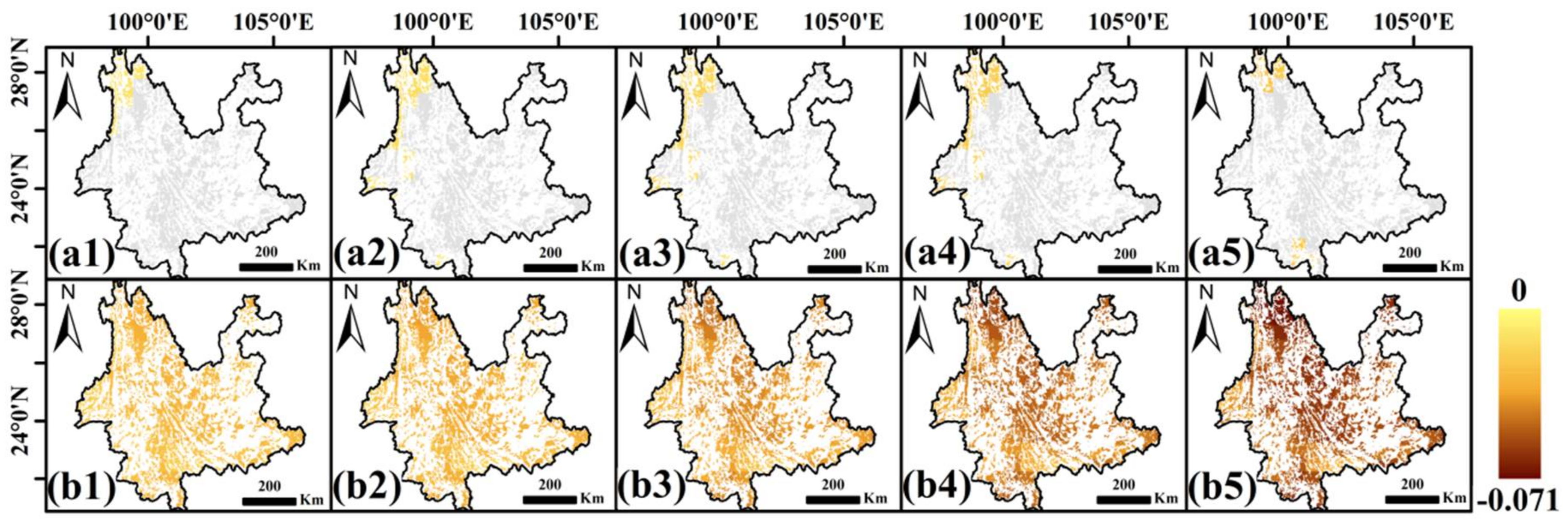
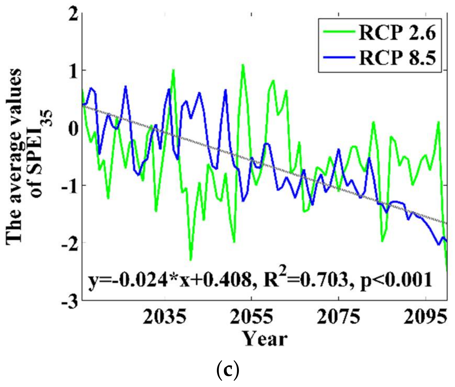
3.4. Stock-Volume-Related Drought Risk in Future

Based on the variations in the SPEI under the different climate change scenarios, a linear regression model was constructed to show the relationship between SPEIopt and dEVI for all groups of forest stock volume density. Next, the variations in dEVIfuture were simulated, and the relative climate change risks facing forests were compared between different forest stock volume densities. The predicted values (dEVIfuture) were affected by the drought stress intensity and by the stock volume (Figure 7a,b). Drought was more severe under the high-concentrations scenario (RCP 8.5) than under the low-concentrations scenario (RCP 2.6). Thus, the dEVIfuture showed a clear downtrend (p < 0.05) under the high-concentrations scenario (Figure 7b), but not under the low-concentrations scenario (p < 0.05) (Figure 7a). On the other hand, the variations in the dEVIfuture—irrespective of the scenario, whether RCP 2.6 or RCP 8.5—were greater when the stock volume density was higher as forests with high stock volume density are more sensitive to moisture levels.
The spatial pattern of the variations in the dEVIfuture (Figure 8) showed that only part of the total area under forests (less than 12% of the total) was affected significantly under the low-concentrations scenario (RCP 2.6): the dEVIfuture for more than 88% of the area under forests (Figure 8(a1–a5)) showed no decrease. However, under the high-concentrations scenario (RCP 8.5), the dEVIfuture decreased markedly over the entire area (p < 0.05) (Figure 8(b1–b5)). Furthermore, the extent of the decrease in the dEVIfuture was related to the increase in forest stock volume density: the higher the forest stock volume density, the greater the decrease in the dEVIfuture.
Thus, as drought becomes more frequent and more intense as a result of global climate change, the risk to forests also increases, particularly under the high-concentrations scenario (RCP 8.5). The effect of drought of a given intensity is greater on forests with high stock volume density, which are thus both more sensitive and more vulnerable.

4. Discussion

4.1. Importance of Optimal Time Scale for SPEI

The length of hysteresis in the forest drought response changes with the type of forest [27,28] as the cumulative effect of water deficit or surplus that will influence forest growth is different for different types of forests [10,28,29]. If the differences in forest attributes are ignored, the SPEI that is assigned artificially on a fixed time scale cannot reflect the differences in the forest drought response accurately, thereby affecting the accuracy of evaluating and predicting such responses. This study constructed linear regression models that expressed the relationship between the SPEI at 1–36 month time scales and the dEVI that reflected the changes of forest growth to choose the optimal model that could best reflect (maximum R2) the relationship between drought and forest growth. Next, to characterize the effect of drought on forest growth and to make the research results more accurate, the index of meteorological drought on the optimal time scale (SPEIopt) was obtained. The length of hysteresis in the forest drought response, the sensitivity of forests to the changes of drought stress intensity, and the degree of forest were all influenced by drought and all increased as the forest stock volume density increased. These results indicated that it is important to select a suitable time scale for the meteorological drought index for different forest attributes. Only in this way can the correlation between a meteorological drought index and an agricultural drought index be constructed effectively. The present research also showed that the length of hysteresis, or the time taken by forests with different stock volume densities to respond to drought, was about 2–3 years in Yunnan Province, a finding consistent with that reported by Orwig and Abrams (1997) [65] and Wu et al. [27].

4.2. Differences in Response Due to Differences in Stock Volume Density

Based on the optimal time scale of SPEI (SPEIopt), it was seen that the length of hysteresis in responding to drought increased as the forest stock volume density increased. One possible reason is that forests with high stock volume density could be older, and old trees can counter meteorological drought by accessing underground water from greater depths (at which moisture from earlier precipitation is stored) [66,67]. On the other hand, forests with low stock volume density could be younger, and the root systems of young trees are shallower, therefore allowing young trees to respond to drought faster [68]. Due to the relatively large reserves of water in forests with high stock volume density, the hysteresis and the cumulative time of water balance that affects forest growth are longer. Based on the statistical model of the relationship between the SPEIopt and the dEVI, the present research showed that the sensitivity of forests to drought increased with the increase in forest stock volume density as the high stock volume density implied a high leaf area index (LAI) and large biomass—and therefore greater water requirements—to maintain regular growth [19]. Forests with high stock volume density could consist of taller trees (the water conduction efficiency of which is also lower than that in shorter trees) that make up forests with low stock volume density [20]. Taller trees are also more prone to xylem embolism, which typically occurs when water is in short supply. In addition, the high density of stock volume could be driven by the high number of small-intermediate stems, which cause the growth of forests with high stock volume density, to stagnate and creates intense competition for water [69]. Above all, given that forests with high stock volume density are more sensitive to drought and have low resistance to drought, they are more likely to be affected by droughts that become more frequent and more severe as a result of global climate change, a link worthy of attention by future forest administrations [63].
The xylem embolism that the research mentioned previously is one of the mechanisms of forest decay (or EVI decrease). The mechanism of forest decay could be xylem embolism, carbon starvation, or both [16,17,18]. Xylem embolism can occur more quickly under very severe drought [16]; however, carbon starvation seems to be the most important factor in determining EVI decrease under long-term climate conditions [16]. Given that Yunnan suffered from long-term and severe droughts during 2001–2014 [10,41,42], both xylem embolism and carbon starvation may occur in Yunnan. This is a hypothesis that is hard to verify through remote sensing alone, so more experimental data are required in the future.

4.3. Difference in Response to Future Climate Change

The forest drought response under the two scenarios depends on the forest stock volume density. Forest growth was affected adversely owing to annual fluctuations in moisture under the low-concentration scenario RCP 2.6, and the scenario showed no marked changes with time (Figure 7a). However, under the high-concentration scenario RCP 8.5, aside from the annual fluctuations, forest growth also decreased markedly over time (Figure 7b). To explore the reasons for the above differences between the two scenarios, the annual average values of the SPEI at different time scales (23, 24, and 35 months) in all regions were compared. Whereas the meteorological drought index under Scenario RCP 2.6 changed little over time (Figure 9), that under Scenario RCP 8.5 decreased markedly over time (Figure 9). This shows that the intensity of drought will increase under the high-concentration scenario, which is the reason for the differences in outcome between the two scenarios, and also the reason for the gradual deterioration of all forest-growing states over time. Forests with a high stock volume density will be affected more than those with a low stock volume density by a drought of a given intensity and will also be more sensitive and vulnerable to it (Figure 7b).

4.4. Uncertainty

A variety of ways were used to reduce uncertainty in the research. To reduce the complicated impacts caused by both biotic and abiotic factors on the EVI itself, the dEVI was constructed at the level of the grid based on EVI. Compared to the EVI, the deficit of EVI (i.e., dEVI) reflected the change of EVI directly related with the environmental stress (e.g., drought), so it was more suitable to build the statistical relationship between the forest drought response to the meteorological drought indexes such as the SPEI, which is also an indicator that reflects the relative change of water deficit or surplus. Second, to improve accuracy, the map showing the distribution of forests of different stock volume density was derived from the Seventh National Forest Resources Inventory. The inventory was compiled over five years, and 0.415 million permanent sample plots were adopted to acquire 0.16 billion groups of basic data [50]. This inventory is the foremost data set on forest resources of China at present. Finally, to reduce the uncertainty of the mode result itself, the arithmetic average of the meteorological data obtained through multiple modes was used in this research.
Despite these efforts, some uncertainties remained. For example, because the limitation of the forest stock volume density maps for each year, the fixed map of 2004–2008 was used for 14 years (2001–2014), and some uncertainties due to timber harvesting or land conversion may possibly exist in the research. Furthermore, as the spatial distribution maps of forest stock volume density are limited in the future scenarios, although it was assumed that the extent of forest cover, the total area was unchanged, and only one of the five grades of stock volume densities, the reality is likely to be different, which adds some uncertainty to the evaluation results. To make the assessment of the impact of drought more precise, we need more reliable data on the distribution of forest stock volume density. In addition, forest fires might impact the research results [70]; however, based on the data of the China forestry statistical yearbook from 2001–2014 [71,72,73,74,75,76,77,78,79,80,81,82,83,84], we found that the percentage of the total area of forest damaged by fire from 2001–2014 was less than 0.17% of the forest area, so the uncertainties driven by forest fires will not change our main conclusions.

5. Conclusions

To reveal the potential impacts of different stock volumes on the forest drought response, forests in Yunnan Province were chosen and the changes in the remote-sensing-enhanced vegetation index (dEVI) were used as representative of the response. The relationships between the meteorological drought index SPEI and dEVI as well as those between the SPEI at the optimal time scale and the dEVI for forests with different stock volume densities were analyzed. A close linear relation existed between the SPEI and the dEVI, but the relation depended on the time scale: at the optimal time scale, the SPEI reflected the effects of drought on forests effectively, and the time scales increased with the increase in forest stock volume density. This meant that if the variation in the time scale of SPEI caused by spatial differences in forest stock volume was ignored, and only the SPEI at a fixed time scale was used for assessing the effects of drought on forests, the results will carry a systematic bias. Based on the synthesis of all the relationships between the SPEI at the optimal time scale and data from remote sensing, it is suggested that forests with a high stock volume density require more water and are therefore, are more sensitive to changes in water deficit and are likely to suffer more in the future following global changes in climate (scenario RCP 8.5).

Acknowledgments

This study was supported by the National Natural Science Foundation of China (41621061 and 41571185), the Fundamental Research Funds for the Central University (2015KJJCB33), and the National Basic Research Program of China (2012CB955401). C.Y. was supported by City University of New York, PSC-CUNY ENHC-48-33 and PSC-CUNY CIRG-80209-08-22.

Author Contributions

H.L. and T.Z. performed the data analysis and drafted the manuscript. C.Y., P.X., X.Z., S.G. and X.L. participated in discussions and provided useful data and comments. All of the authors contributed to the manuscript and approved the final version.

Conflicts of Interest

The authors declare that they have no conflicts of interest.

References

  1. Dixon, R.K.; Brown, S.; Houghton, R.A.; Solomon, A.M.; Trexler, M.C.; Wisniewski, J. Carbon pools and flux of global forest ecosystems. Science 1994, 263, 185–190. [Google Scholar] [CrossRef] [PubMed]
  2. Jackson, R.B.; Jobbagy, E.G.; Avissar, R.; Roy, S.B.; Barrett, D.J.; Cook, C.W.; Farley, K.A.; le Maitre, D.C.; McCarl, B.A.; Murray, B.C. Trading water for carbon with biological sequestration. Science 2005, 310, 1944–1947. [Google Scholar] [CrossRef] [PubMed]
  3. McKinley, D.C.; Ryan, M.G.; Birdsey, R.A.; Giardina, C.P.; Harmon, M.E.; Heath, L.S.; Houghton, R.A.; Jackson, R.B.; Morrison, J.F.; Murray, B.C.; et al. A synthesis of current knowledge on forests and carbon storage in the United States. Ecol. Appl. 2011, 21, 1902–1924. [Google Scholar] [CrossRef] [PubMed]
  4. Cook, B.I.; Smerdon, J.E.; Seager, R.; Coats, S. Global warming and 21st century drying. Clim. Dyn. 2014, 43, 2607–2627. [Google Scholar] [CrossRef]
  5. Dai, A. Increasing drought under global warming in observations and models. Nat. Clim. Chang. 2013, 3, 52–58. [Google Scholar] [CrossRef]
  6. Allen, C.D.; Macalady, A.K.; Chenchouni, H.; Bachelet, D.; McDowell, N.; Vennetier, M.; Kitzberger, T.; Rigling, A.; Breshears, D.D.; Hogg, E.H.; et al. A global overview of drought and heat-induced tree mortality reveals emerging climate change risks for forests. For. Ecol. Manag. 2010, 259, 660–684. [Google Scholar] [CrossRef]
  7. Huang, S.; Krysanova, V.; Hattermann, F. Projections of climate change impacts on floods and droughts in Germany using an ensemble of climate change scenarios. Reg. Environ. Chang. 2015, 15, 461–473. [Google Scholar] [CrossRef]
  8. Choat, B.; Jansen, S.; Brodribb, T.J.; Cochard, H.; Delzon, S.; Bhaskar, R.; Bucci, S.J.; Feild, T.S.; Gleason, S.M.; Hacke, U.G.; et al. Global convergence in the vulnerability of forests to drought. Nature 2012, 491, 752. [Google Scholar] [CrossRef] [PubMed]
  9. Xu, C.; Liu, H.; Anenkhonov, O.A.; Korolyuk, A.Y.; Sandanov, D.V.; Balsanova, L.D.; Naidanov, B.B.; Wu, X. Long-term forest resilience to climate change indicated by mortality, regeneration, and growth in semiarid southern siberia. Glob. Chang. Biol. 2017, 23, 2370–2382. [Google Scholar] [CrossRef] [PubMed]
  10. Luo, H.; Zhou, T.; Wu, H.; Zhao, X.; Wang, Q.; Gao, S.; Li, Z. Contrasting responses of planted and natural forests to drought intensity in Yunnan, China. Remote Sens. 2016, 8, 635. [Google Scholar] [CrossRef]
  11. Goetz, R.; Cañizares, C.; Pujol, J.; Xabadia, A. Forest management and biodiversity in size-structured forests under climate change. In Dynamic Optimization in Environmental Economics; Springer: Berlin/Heidelberg, Germany, 2014; Volume 15, pp. 265–286. [Google Scholar]
  12. Walsh, D.; Rossi, S.; Lord, D. Size and age: Intrinsic confounding factors affecting the responses to a water deficit in black spruce seedlings. iFor. Biogeosci. For. 2015, 8, 401–409. [Google Scholar] [CrossRef]
  13. Grossnickle, S.C.; Folk, R.S. Stock quality assessment: Forecasting survival or performance on a reforestation site. Tree Plant. Notes 1993, 44, 113–121. [Google Scholar]
  14. Sperry, J.S.; Hacke, U.G.; Oren, R.; Comstock, J.P. Water deficits and hydraulic limits to leaf water supply. Plant Cell Environ. 2002, 25, 251–263. [Google Scholar] [CrossRef] [PubMed]
  15. Brodribb, T.J.; Cochard, H. Hydraulic failure defines the recovery and point of death in water-stressed conifers. Plant Physiol. 2009, 149, 575–584. [Google Scholar] [CrossRef] [PubMed]
  16. McDowell, N.; Pockman, W.T.; Allen, C.D.; Breshears, D.D.; Cobb, N.; Kolb, T.; Plaut, J.; Sperry, J.; West, A.; Williams, D.G.; et al. Mechanisms of plant survival and mortality during drought: Why do some plants survive while others succumb to drought? New Phytol. 2008, 178, 719–739. [Google Scholar] [CrossRef] [PubMed]
  17. McDowell, N.G. Mechanisms linking drought, hydraulics, carbon metabolism, and vegetation mortality. Plant Physiol. 2011, 155, 1051–1059. [Google Scholar] [CrossRef] [PubMed]
  18. Sevanto, S.; McDowell, N.G.; Dickman, L.T.; Pangle, R.; Pockman, W.T. How do trees die? A test of the hydraulic failure and carbon starvation hypotheses. Plant Cell Environ. 2014, 37, 153–161. [Google Scholar] [CrossRef] [PubMed]
  19. Midgley, J.J. Is bigger better in plants? The hydraulic costs of increasing size in trees. Trends Ecol. Evol. 2003, 18, 5–6. [Google Scholar] [CrossRef]
  20. Koch, G.W.; Sillett, S.C.; Jennings, G.M.; Davis, S.D. The limits to tree height. Nature 2004, 428, 851–854. [Google Scholar] [CrossRef] [PubMed]
  21. Rijkers, T.; Pons, T.L.; Bongers, F. The effect of tree height and light availability on photosynthetic leaf traits of four neotropical species differing in shade tolerance. Funct. Ecol. 2000, 14, 77–86. [Google Scholar] [CrossRef]
  22. Yoder, B.J.; Ryan, M.G.; Waring, R.H.; Schoettle, A.W.; Kaufmann, M.R. Evidence of reduced photosynthetic rates in old trees. For. Sci. 1994, 40, 513–527. [Google Scholar]
  23. Hubbard, R.M.; Bond, B.J.; Ryan, M.G. Evidence that hydraulic conductance limits photosynthesis in old pinus ponderosa trees. Tree Physiol. 1999, 19, 165–172. [Google Scholar] [CrossRef] [PubMed]
  24. Carlos Linares, J.; Taiqui, L.; Sangueesa-Barreda, G.; Ignacio Seco, J.; Julio Camarero, J. Age-related drought sensitivity of atlas cedar (Cedrus atlantica) in the moroccan middle atlas forests. Dendrochronologia 2013, 31, 88–96. [Google Scholar] [CrossRef]
  25. Bond, B.J. Age-related changes in photosynthesis of woody plants. Trends Plant Sci. 2000, 5, 349–353. [Google Scholar] [CrossRef]
  26. Wu, D.; Zhao, X.; Liang, S.; Zhou, T.; Huang, K.; Tang, B.; Zhao, W. Time-lag effects of global vegetation responses to climate change. Glob. Chang. Biol. 2015, 21, 3520–3531. [Google Scholar] [CrossRef] [PubMed]
  27. Wu, X.; Liu, H.; Li, X.; Ciais, P.; Babst, F.; Guo, W.; Zhang, C.; Magliulo, V.; Pavelka, M.; Liu, S.; et al. Differentiating drought legacy effects on vegetation growth over the temperate northern hemisphere. Glob. Chang. Biol. 2017, 24, 504–516. [Google Scholar] [CrossRef] [PubMed]
  28. Huang, K.; Yi, C.; Wu, D.; Zhou, T.; Zhao, X.; Blanford, W.J.; Wei, S.; Wu, H.; Ling, D.; Li, Z. Tipping point of a conifer forest ecosystem under severe drought. Environ. Res. Lett. 2015, 10, 024011. [Google Scholar] [CrossRef]
  29. Li, Z.; Zhou, T.; Zhao, X.; Huang, K.; Gao, S.; Wu, H.; Luo, H. Assessments of drought impacts on vegetation in china with the optimal time scales of the climatic drought index. Int. J. Environ. Res. Public Health 2015, 12, 7615–7634. [Google Scholar] [CrossRef] [PubMed]
  30. Palmer, W. Meteorological Drought; US Department of Commerce Weather Bureau: Washington, DC, USA, 1965.
  31. Mckee, T.B.; Doesken, N.J.; Kleist, J. The relationship of drought frequency and duration to time scales. In Proceedings of the 8th Conference on Applied Climatology, Anaheim, CA, USA, 17–22 January 1993. [Google Scholar]
  32. Vicente-Serrano, S.M.; Begueria, S.; Lopez-Moreno, J.I. A multiscalar drought index sensitive to global warming: The standardized precipitation evapotranspiration index. J. Clim. 2010, 23, 1696–1718. [Google Scholar] [CrossRef]
  33. Huete, A.; Didan, K.; Miura, T.; Rodriguez, E.P.; Gao, X.; Ferreira, L.G. Overview of the radiometric and biophysical performance of the modis vegetation indices. Remote Sens. Environ. 2002, 83, 195–213. [Google Scholar] [CrossRef]
  34. Potop, V.; Mozny, M.; Soukup, J. Drought evolution at various time scales in the lowland regions and their impact on vegetable crops in the Czech Republic. Agric. For. Meteorol. 2012, 156, 121–133. [Google Scholar] [CrossRef]
  35. Mavromatis, T. Drought index evaluation for assessing future wheat production in Greece. Int. J. Climatol. 2007, 27, 911–924. [Google Scholar] [CrossRef]
  36. Feng, S.; Trnka, M.; Hayes, M.; Zhang, Y. Why do different drought indices show distinct future drought risk outcomes in the US Great Plains? J. Clim. 2017, 30, 265–278. [Google Scholar] [CrossRef]
  37. Vicente-Serrano, S.M.; Begueria, S.; Lopez-Moreno, J.I. Comment on “characteristics and trends in various forms of the palmer drought severity index (PDSI) during 1900–2008” by Aiguo Dai. J. Geophys. Res.-Atmos. 2011, 116. [Google Scholar] [CrossRef]
  38. Zhao, X.; Wei, H.; Liang, S.; Zhou, T.; He, B.; Tang, B.; Wu, D. Responses of natural vegetation to different stages of extreme drought during 2009–2010 in southwestern china. Remote Sens. 2015, 7, 14039–14054. [Google Scholar] [CrossRef]
  39. State Forestry Administration of the People’s Republic of China. The Main Results at Eighth National Forest Resources Inventory (2009–2013). 2015. Available online: http://www.forestry.gov.cn/main/65/content-659670.html (accessed on 4 April 2018).
  40. The State Forestry Bureau. Atlas of Forest Resoureces of China; China Forestry Publishing House: Beijing, China, 2010. [Google Scholar]
  41. Chen, H.-P.; Jia, G.-S.; Feng, J.-M.; Dong, Y.-S. Increased browning of woody vegetation due to continuous seasonal droughts in Yunnan province, China. Atmos. Ocean. Sci. Lett. 2014, 7, 120–125. [Google Scholar]
  42. Yan, Z.; Zhang, Y.; Zhou, Z.; Han, N. The spatio-temporal variability of droughts using the standardized precipitation index in Yunnan, China. Nat. Hazards 2017, 88, 1023–1042. [Google Scholar] [CrossRef]
  43. Abbas, S.; Nichol, J.E.; Qamer, F.M.; Xu, J. Characterization of drought development through remote sensing: A case study in central Yunnan, China. Remote Sens. 2014, 6, 4998–5018. [Google Scholar] [CrossRef]
  44. Xu, P.; Zhou, T.; Zhao, X.; Luo, H.; Gao, S.; Li, Z.; Cao, L. Diverse responses of different structured forest to drought in southwest china through remotely sensed data. Int. J. Appl. Earth Obs. Geoinf. 2018, 69, 217–225. [Google Scholar] [CrossRef]
  45. The Centre for Environmental Data Analysis. Available online: http://data.ceda.ac.uk/badc/cru/data/cru_ts/ (accessed on 4 April 2018).
  46. The Climatic Research Unit of the University of East Anglia. Available online: http://digital.csic.es/handle/10261/128892 (accessed on 4 April 2018).
  47. Guo, Z.D.; Hu, H.F.; Li, P.; Li, N.Y.; Fang, J.Y. Spatio-temporal changes in biomass carbon sinks in china’s forests from 1977 to 2008. Sci. Chin. Life Sci. 2013, 7, 661–671. [Google Scholar] [CrossRef] [PubMed]
  48. Pilli, R.; Grassi, G.; Kurz, W.A.; Smyth, C.E.; Blujdea, V. Application of the cbm-cfs3 model to estimate Italy’s forest carbon budget, 1995–2020. Ecol. Model. 2013, 266, 144–171. [Google Scholar] [CrossRef]
  49. King, D.A. The adaptive significance of tree height. Am. Nat. 1990, 135, 809–828. [Google Scholar] [CrossRef]
  50. Forest Resources Management Department of the State Forestry Administration. Forest Resources Statistics of China—The Seventh National Forest Resources Inventory China; Forest Resources Management Department of the State Forestry Administration: Beijing, China, 2010.
  51. Maeda, E.E.; Heiskanen, J.; Aragao, L.E.O.C.; Rinne, J. Can modis evi monitor ecosystem productivity in the amazon rainforest? Geophys. Res. Lett. 2014, 41, 7176–7183. [Google Scholar] [CrossRef]
  52. The Land Processes Distributed Active Archive Center. Available online: http://reverb.echo.nasa.gov/reverb/#utf8=%E2%9C%93spatial_type=rectangle (accessed on 4 April 2018).
  53. Holben, B.N. Characteristics of maximum-value composite images from temporal avhrr data. Int. J. Remote Sens. 1986, 7, 1417–1434. [Google Scholar] [CrossRef]
  54. Garroutte, E.L.; Hansen, A.J.; Lawrence, R.L. Using ndvi and evi to map spatiotemporal variation in the biomass and quality of forage for migratory elk in the greater yellowstone ecosystem. Remote Sens. 2016, 8, 404. [Google Scholar] [CrossRef]
  55. Vicente-Serrano, S.M.; Gouveia, C.; Julio Camarero, J.; Begueria, S.; Trigo, R.; Lopez-Moreno, J.I.; Azorin-Molina, C.; Pasho, E.; Lorenzo-Lacruz, J.; Revuelto, J.; et al. Response of vegetation to drought time-scales across global land biomes. Proc. Natl. Acad. Sci. USA 2013, 110, 52–57. [Google Scholar] [CrossRef] [PubMed] [Green Version]
  56. Guttman, N.B. Comparing the palmer drought index and the standardized precipitation index. J. Am. Water Resour. Assoc. 1998, 34, 113–121. [Google Scholar] [CrossRef]
  57. Dunne, J.P.; John, J.G.; Shevliakova, E.; Stouffer, R.J.; Krasting, J.P.; Malyshev, S.L.; Milly, P.C.D.; Sentman, L.T.; Adcroft, A.J.; Cooke, W.; et al. GFDL’S ESM2 global coupled climate-carbon earth system models. Part II: Carbon system formulation and baseline simulation characteristics. J. Clim. 2013, 26, 2247–2267. [Google Scholar] [CrossRef]
  58. Dufresne, J.L.; Foujols, M.A.; Denvil, S.; Caubel, A.; Marti, O.; Aumont, O.; Balkanski, Y.; Bekki, S.; Bellenger, H.; Benshila, R.; et al. Climate change projections using the IPSL-CM5 earth system model: From CMIP3 to CMIP5. Clim. Dyn. 2013, 40, 2123–2165. [Google Scholar] [CrossRef] [Green Version]
  59. Watanabe, S.; Hajima, T.; Sudo, K.; Nagashima, T.; Takemura, T.; Okajima, H.; Nozawa, T.; Kawase, H.; Abe, M.; Yokohata, T.; et al. MIROC-ESM 2010: Model description and basic results of CMIP5-20c3m experiments. Geosci. Model Dev. 2011, 4, 845–872. [Google Scholar] [CrossRef]
  60. Bentsen, M.; Bethke, I.; Debernard, J.B.; Iversen, T.; Kirkevag, A.; Seland, O.; Drange, H.; Roelandt, C.; Seierstad, I.A.; Hoose, C.; et al. The Norwegian earth system model, NorESM1-M—Part 1: Description and basic evaluation of the physical climate. Geosci. Model Dev. 2013, 6, 687–720. [Google Scholar] [CrossRef]
  61. Chen, H.; Sun, J. Changes in drought characteristics over china using the standardized precipitation evapotranspiration index. J. Clim. 2015, 28, 5430–5447. [Google Scholar] [CrossRef]
  62. The SPEI Calculation Procedure. Available online: http://digital.csic.es/handle/10261/10002 (accessed on 14 April 2018).
  63. Bellassen, V.; Luyssaert, S. Managing forests in uncertain times. Nature 2014, 506, 153–155. [Google Scholar] [CrossRef] [PubMed]
  64. Paulo, A.A.; Rosa, R.D.; Pereira, L.S. Climate trends and behaviour of drought indices based on precipitation and evapotranspiration in Portugal. Nat. Hazards Earth Syst. Sci. 2012, 12, 1481–1491. [Google Scholar] [CrossRef] [Green Version]
  65. Orwig, D.A.; Abrams, M.D. Variation in radial growth responses to drought among species, site, and canopy strata. Trees-Struct. Funct. 1997, 11, 474–484. [Google Scholar] [CrossRef]
  66. Gazis, C.; Feng, X.H. A stable isotope study of soil water: Evidence for mixing and preferential flow paths. Geoderma 2004, 119, 97–111. [Google Scholar] [CrossRef]
  67. Mahmood, T.H.; Vivoni, E.R. Forest ecohydrological response to bimodal precipitation during contrasting winter to summer transitions. Ecohydrology 2014, 7, 998–1013. [Google Scholar] [CrossRef]
  68. Sala, O.E.; Lauenroth, W.K.; Parton, W.J. Long-term soil-water dynamics in the shortgrass steppe. Ecology 1992, 73, 1175–1181. [Google Scholar] [CrossRef]
  69. Lechuga, V.; Carraro, V.; Viñegla, B.; Carreira, J.A.; Linares, J.C. Managing drought-sensitive forests under global Change. Low competition enhances long-term growth and water uptake in abies pinsapo. For. Ecol. Manag. 2017, 406, 72–82. [Google Scholar] [CrossRef]
  70. Zhang, C.; Ju, W.; Chen, J.M.; Wang, X.; Yang, L.; Zheng, G. Disturbance-induced reduction of biomass carbon sinks of china’s forests in recent years. Environ. Res. Lett. 2015, 11, 114021. [Google Scholar] [CrossRef]
  71. The State Forestry Bureau. China Forestry Statistial Yearbook 2001; China Forestry Publishing House: Beijing, China, 2002. [Google Scholar]
  72. The State Forestry Bureau. China Forestry Statistial Yearbook 2002; China Forestry Publishing House: Beijing, China, 2003. [Google Scholar]
  73. The State Forestry Bureau. China Forestry Statistial Yearbook 2003; China Forestry Publishing House: Beijing, China, 2004. [Google Scholar]
  74. The State Forestry Bureau. China Forestry Statistial Yearbook 2004; China Forestry Publishing House: Beijing, China, 2005. [Google Scholar]
  75. The State Forestry Bureau. China Forestry Statistial Yearbook 2005; China Forestry Publishing House: Beijing, China, 2006. [Google Scholar]
  76. The State Forestry Bureau. China Forestry Statistial Yearbook 2006; China Forestry Publishing House: Beijing, China, 2007. [Google Scholar]
  77. The State Forestry Bureau. China Forestry Statistial Yearbook 2007; China Forestry Publishing House: Beijing, China, 2008. [Google Scholar]
  78. The State Forestry Bureau. China Forestry Statistial Yearbook 2008; China Forestry Publishing House: Beijing, China, 2009. [Google Scholar]
  79. The State Forestry Bureau. China Forestry Statistial Yearbook 2009; China Forestry Publishing House: Beijing, China, 2010. [Google Scholar]
  80. The State Forestry Bureau. China Forestry Statistial Yearbook 2010; China Forestry Publishing House: Beijing, China, 2011. [Google Scholar]
  81. The State Forestry Bureau. China Forestry Statistial Yearbook 2011; China Forestry Publishing House: Beijing, China, 2012. [Google Scholar]
  82. The State Forestry Bureau. China Forestry Statistial Yearbook 2012; China Forestry Publishing House: Beijing, China, 2013. [Google Scholar]
  83. The State Forestry Bureau. China Forestry Statistial Yearbook 2013; China Forestry Publishing House: Beijing, China, 2014. [Google Scholar]
  84. The State Forestry Bureau. China Forestry Statistial Yearbook 2014; China Forestry Publishing House: Beijing, China, 2015. [Google Scholar]
Figure 1. Distribution of forest stock volume densities in Yunnan province, China [40].
Forests 09 00209 g001
Figure 2. The spatial distribution of (a) the mean annual precipitation and (b) the mean annual temperature from 2001–2014. These data sets (CRU, the Climatic Research Unit, TS 3.23) were obtained from the Center for Environmental Data Analysis [45], which forms the basis of CRU SPEIbase (v2.4) [46].
Forests 09 00209 g002
Figure 3. The spatial distribution of (a) the mean annual of EVI and (b) the annual standard deviation of EVI from 2001–2014. The EVI data were only for July in each year.
Forests 09 00209 g003
Figure 4. Correlation between dEVI and the SPEI at different time scales for forests with five groups of stock volume density (m3·ha−1): (a) <30; (b) 30–60; (c) 60–90; (d) 90–120; and (e) ≥120. The green highlight shows significance at the level of 0.01.
Forests 09 00209 g004aForests 09 00209 g004b
Figure 5. Sensitivity to drought of forests of varying stock volume densities.
Forests 09 00209 g005
Figure 6. Potential simulation error in SPEI at fixed time scales that ignored the effect of forest stock volume.
Forests 09 00209 g006
Figure 7. Changes in annual average dEVIfuture of forests under two future climate scenarios. (a) RCP 2.6; and (b) RCP 8.5.
Forests 09 00209 g007
Figure 8. Pattern of spatial variation in the coefficient of the temporal variation trend of dEVIfuture following global climate change. (a1a5) show the coefficients of <30, 30–60, 60–90, 90–120, and ≥120 (m3·ha−1), respectively, at every spatial grid in the climatic scenario of RCP 2.6, and the proportion of grids at the significance level of 0.05 to the total number of grids was 6.8% in the case of densities below 30 m3·ha−1, 11.5% in each of the next three categories, and 5.7% in the case of densities greater than or equal to 120 m3·ha−1; (b1b5) show the corresponding values under Scenario RCP 8.5.
Forests 09 00209 g008
Figure 9. Changes in SPEI over time under scenarios RCP 2.6 and RCP 8.5 on time scales of (a) 23 months; (b) 24 months; and (c) 35 months. The 24 months represent the optimal time scale of SPEI for the three groups of stock volume density: 30–60, 60–90, 90–120 m3·ha−1.
Forests 09 00209 g009aForests 09 00209 g009b
Table 1. Eight grades of drought and their corresponding SPEI values.
Drought Stress IntensitySPEI
Severe drought≤−1.5
Moderate drought−1.5 to ≤−1
Mild drought−1 to ≤−0.5
Normal (−)−0.5 to ≤0
Normal (+)0 to ≤0.5
Mild wet0.5 to ≤1
Moderate wet1 to ≤1.5
Severe wet>1.5
The grades in this table are a modified version of those reported by Paulo et al. [64], and the proportion of forest grids in each grade to the total number of grids exceeded 5%.
Table 2. Optimal models of SPEI and dEVI for different forest stock volume densities.
Forest Stock Volume Density (m3·ha−1)<3030–6060–9090–120≥120
The optimal time scale of SPEI (month)2324242435
Regression coefficient1.351.581.972.352.88
constant−18.28−18.82−19.52−19.84−21.19
R2max0.770.800.850.960.99
p value<0.001<0.001<0.001<0.001<0.001

