Estimation of Total Biomass in Aleppo Pine Forest Stands Applying Parametric and Nonparametric Methods to Low-Density Airborne Laser Scanning Data

Abstract

The account of total biomass can assist with the evaluation of climate regulation policies from local to global scales. This study estimates total biomass (TB), including tree and shrub biomass fractions, in Pinus halepensis Miller forest stands located in the Aragon Region (Spain) using Airborne Laser Scanning (ALS) data and fieldwork. A comparison of five selection methods and five regression models was performed to relate the TB, estimated in 83 field plots through allometric equations, to several independent variables extracted from ALS point cloud. A height threshold was used to include returns above 0.2 m when calculating ALS variables. The sample was divided into training and test sets composed of 62 and 21 plots, respectively. The model with the lower root mean square error (15.14 tons/ha) after validation was the multiple linear regression model including three ALS variables: the 25th percentile of the return heights, the variance, and the percentage of first returns above the mean. This study confirms the usefulness of low-density ALS data to accurately estimate total biomass, and thus better assess the availability of biomass and carbon content in a Mediterranean Aleppo pine forest.

1. Introduction

Forest ecosystems and their associated understory act as important carbon sinks, providing habitats for wildlife [1,2] and promoting economic and social services to societies [3,4]. The sequestration of carbon and CO₂ by forest biomass and soils plays a major role in managing greenhouse gas emissions [5] providing a low-cost opportunity in climate policies [6]. The estimation of tree and shrub biomass in the Mediterranean Basin also contributes to better understanding fire behavior, which constitutes one of the most relevant disturbances as well as being a source of greenhouse gas emission to the atmosphere [7,8,9,10,11]. The inclusion of understory vegetation in carbon sequestration has been traditionally ignored [12] since it represents lower amounts of biomass compared with tree aboveground biomass (AGB). However, considering the global scale this amount constitutes an important pool for carbon sequestration [12,13].

Remote sensing technologies have demonstrated effectiveness for estimating forest resources such as biomass [14,15]. Particularly, Airborne Laser Scanning (ALS) is currently considered one of the best tools due to its capability to provide 3-D information of vegetation structure. Vertical forest structure has been estimated with ALS data for several applications, such as forest inventory [16,17,18], forest structural heterogeneity [19,20,21,22], fuel type mapping [23,24] fuel modelling [23,24,25,26] or tree damage detection after natural disasters [27,28,29] for several height strata. However, few studies have focused on shrub biomass characterization with ALS data [30,31,32,33]. Some studies have used low density ALS data to estimate forest biomass [25,34,35,36,37,38], but little research has been performed including shrub vegetation because of the inherent difficulty in the estimation related to its low height and uniform surface [30]. Several studies state that ALS data tends to underestimate shrub vegetation [39,40,41,42]. Besides, when shrub and tree vegetation cover is high [43] and density of ALS data is low, the accuracy of digital elevation models (DEM) used to normalize return heights decreases [30]. The performed studies use an approach that combines ALS data and harvesting field measurements for biomass estimation [30,33]. In this sense, the lack of more studies to characterize shrub vegetation might have been associated with the necessary destructive sampling to generate forest structure equations, the assumption of simple geometric shapes [44,45], and the additional difficulty to estimate biomass at a regional scale using low-density ALS data. However, the presence of shrub biomass in the understory or the existence of shrubland areas constitutes an important land use in the Mediterranean basin. In this sense, the availability of shrub allometric equations for the main Spanish shrub species [46] have opened new opportunities. These equations allow the estimation of shrub biomass from simple field measurements, such as height and percentage cover per species or group of species. Thus, an area-based approach could be used to estimate biomass, using larger field plots (15 m radius) than traditional ones (1.5 m radius). This approach seems to be less affected by low-density ALS data, as has been proven in accurately estimating forest structure parameters in heterogeneous forests [47].

Few studies have compared different selection methods for ALS modelling [48,49]. In this sense, LASSO selection and the varimax rotation for Principal component analysis (PCA) selection are proposed as novel selection processes for biomass estimation. Some studies have compared different regression models to estimate forest parameters using high point cloud density [16,34,50,51,52], but only Li et al. [33] have compared two regression models to estimate shrub biomass.

The main objective of this study is to estimate the total biomass (TB) in heterogeneous Pinus halepensis Miller (hereinafter Aleppo pine) forest stands located in the Aragón Region (Spain). In this manuscript, TB refers to the dry weight of the plant material from trees, including roots, stems, bark, branches, and leaves from the ground to the apex, as well as the aboveground plant material from shrubs. The values of TB are expressed per unit area in terms of density, i.e., tons of TB per hectare (tons/ha). Specifically, we aim to (1) examine the relationship between biomass calculated at the field plot using allometric equations and ALS-derived variables; and (2) compare five variable selection methods and five different regression models, including regression trees and machine learning algorithms. This paper is organized in five sections. Section 2 describes the processing of ALS and field data, the selection methods, the regression models applied, as well as, the model comparison and validation methods used. Section 3 presents the results including the best TB model. Section 4 describes the discussion of the results and the paper’s conclusions are included in Section 5.

2. Materials and Methods

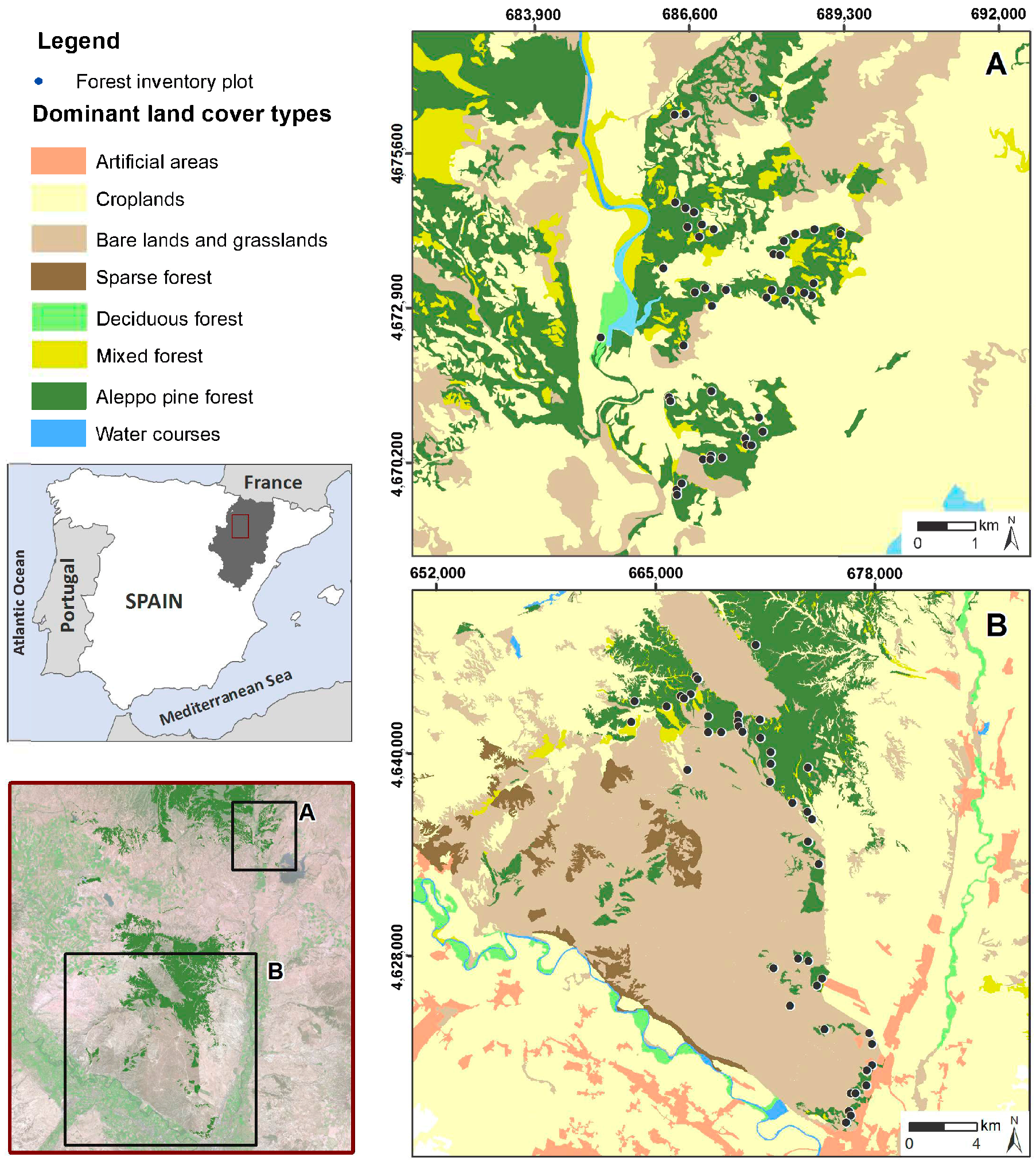
2.1. Study Area

The Aleppo pine forests under study are located in the Ebro Basin (Figure 1), in Northeast Spain. This species represents almost 50% of the forested tree area in Aragón and is well adapted to Mediterranean environmental conditions. The two selected areas (Figure 1) are representative of the Aleppo pine forest in Central Ebro Valley, occupying 11,400 ha.

Climate of the region is Mediterranean with continental features. The average annual temperature is ≈13 °C, ranging from winter mean temperatures lower than 6 °C, to summer mean temperatures of ≈21 °C. Annual precipitation is medium-low and irregular, averaging 455 mm and mostly occurring in autumn and spring [53].

Aleppo pine forests are characterized by a hilly topography, with elevations ranging from 300 to 1150 m above sea level and slopes from 0° to 39°. The lithology of the study area varies from Miocene shales and sandstones, alternating with conglomerates in area A (Figure 1A) to Miocene carbonate and marl sediments in area B (Figure 1B).

Most of these pine stands are semi-natural, although some stands located in the south-eastern part of the area B (Figure 1B) were planted approximately forty years ago. The evergreen understory includes species such as Quercus ilex subsp. rotundifolia, Quercus coccifera, Juniperus oxycedrus, Buxus sempervirens, Juniperus phoenicea, Rosmarinus officinalis, and Thymus vulgaris.

2.2. ALS Data

The ALS data were collected by the Spanish National Plan for Aerial Orthophotography (PNOA) and captured in several surveys carried out between January and February 2011. An airborne Leica ALS60 discrete-return sensor with a small-footprint oscillating-mirror was used. The sensor was operated at a wavelength of 1.064 μm and a scan angle of ±29° from nadir. Data were provided by the National Geographic Information Centre (CNIG) in 2 × 2 km tiles of raw data points in LAS binary files format v. 1.2. The geodetic reference system for x, y, and z coordinates was ETRS 1989 UTM Zone 30 N and heights were orthometrically corrected. The point cloud was captured with up to four returns measured per pulse. The point cloud density was 1.5 point/m², considering all returns with a vertical accuracy better than 0.2 m.

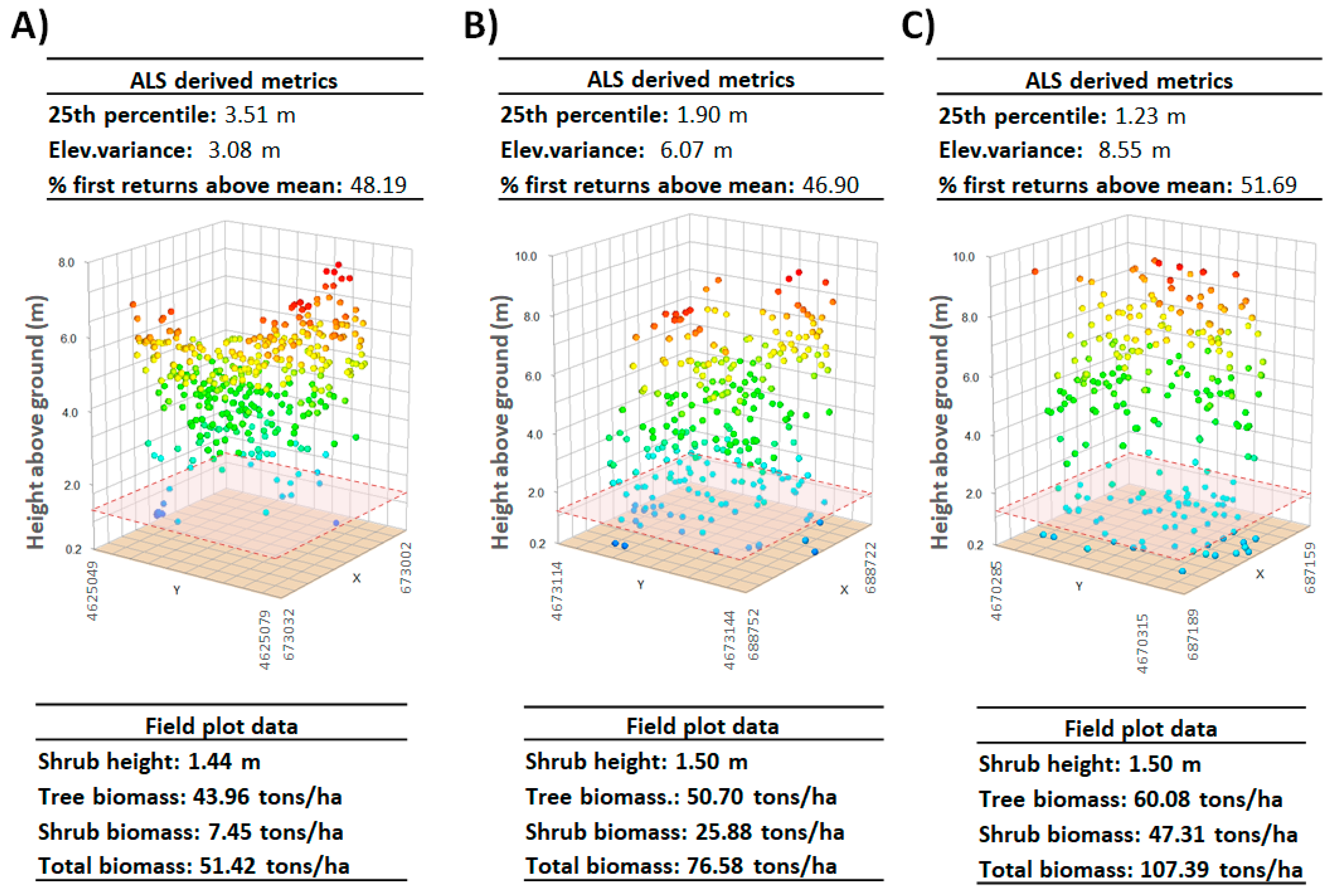
2.3. Field Plot Data and Conversion of Biomass Measurements to ALS Campaign Year

Field data were acquired in 83 circular plots, 15 m radius, at the two study areas (Figure 1). The sampling data fulfil the statistical requirements [55] and consider the size of the study area and the variability of pine forest in terms of canopy cover (CC), canopy height, and terrain slope [56]. The 45 field plots located in area A were collected from June to July 2015 and the 38 field plots located in area B were collected from July to September 2014. A stratified random sampling technique was selected to establish the location of the field plots, considering a representative sample of the tree density, forest structure [47], and terrain variability [57]. To perform this procedure, tree height (h), CC and terrain slopes of the study area were derived from ALS point cloud to define homogeneous areas.

The center of the designated circular plots was located in the field using a Leica VIVA^® GS15 CS10 GNSS real-time kinematic Global Positioning System. The average accuracy of the planimetric coordinates was 0.16 m. The green crown height and h parameter were measured using a Haglöf Sweden^® Vertex instrument and the tree diameter at breast height (dbh) was measured at 1.3 m, using a Haglöf Sweden^® Mantax Precision Blue diameter calliper. Trees with a dbh larger than 7.5 cm were measured in each plot, and trees with a dbh lower than 7.5 cm were only counted. The percentage of canopy cover was estimated, as well as the average height of the different shrub species and the understory coverage.

The temporal lag between ALS acquisition data and field work campaign was 3 and 4 years in area B and area A, respectively. Although no significant changes took place in the study area in that period, field plot data were transformed to match the ALS campaign year. For this purpose, the values of dbh and height growth per diametric class provided by the National Forest Inventory (NFI) were used. These refer to the difference of years between the second NFI (NFI2) and the third one (NFI3), which is eleven years. A linear interpolation based on stand tables was made to estimate the variation between field data and ALS data acquisition (

Table 1. Values of tree diameter at breast height (dbh) and height growth between the second National Forest Inventory (NFI2) and the third one (NFI3) (11 years) and subtractive values of dbh and height when applying linear interpolated degrowth to match Airborne Laser Scanning (ALS) year.

Diametric Class (cm)	dbh Growth (mm)	Height Growth (m)	Area A		Area B
			dbh (mm)	Height (m)	dbh (mm)	Height (m)
<10	24	1.20	−6.55	−0.33	−8.73	−0.44
10–15	29	1.40	−7.91	−0.38	−10.55	−0.51
15–20	33	1.50	−9.00	−0.41	−12.00	−0.55
20–25	30	1.40	−8.18	−0.38	−10.91	−0.51
25–30	30	1.40	−8.18	−0.38	−10.91	−0.51
30–35	33	1.10	−9.00	−0.30	−12.00	−0.40
35–40	32	1.50	−8.73	−0.41	−11.64	−0.55
40–45	27	1.60	−7.36	−0.44	−9.82	−0.58
45–50	24	1.90	−6.55	−0.52	−8.73	−0.69
50–55	58	1.00	−15.82	−0.27	−21.09	−0.36
55–60	10	0.50	−2.73	−0.14	−3.64	−0.18

).

Total tree biomass fractions were calculated using the Pinus halepensis allometric equations according to Ruiz-Peinado et al. [58] (Equations (1)–(5)):

$$\begin{gathered} {\mathrm{W}}_{\mathrm{s}}\left(\mathrm{kg}\right)=0.0139\times {\mathrm{dbh}}^2\times \mathrm{h} \\ {\mathrm{W}}_{\mathrm{b}7}\left(\mathrm{kg}\right)=3.926\times (\mathrm{dbh}-27.5)\times \mathrm{Z}; \end{gathered}$$

(1)

$$\mathrm{If} \mathrm{dbh}\le 27.5 \mathrm{cm} \mathrm{then} \mathrm{Z}=0; \mathrm{If} \mathrm{dhb}>27.5 \mathrm{cm} \mathrm{then} \mathrm{Z}=1$$

(2)

$${\mathrm{W}}_{\mathrm{b}2-7}\left(\mathrm{kg}\right)=4.257+0.00506\times {\mathrm{dbh}}^2\times \mathrm{h}-0.0722\times \mathrm{dbh}\times \mathrm{h}$$

(3)

$${\mathrm{W}}_{\mathrm{b}2+\mathrm{n}}\left(\mathrm{kg}\right)=6.197+0.00932\times {\mathrm{dbh}}^2\times \mathrm{h}-0.0686\times \mathrm{dbh}\times \mathrm{h}$$

(4)

$${\mathrm{W}}_{\mathrm{r}}\left(\mathrm{kg}\right)=0.0785\times {\mathrm{dbh}}^2$$

(5)

where W_s is the biomass weight of the stem fraction, W_b7 is the biomass weight of the thick branch fraction (diameter larger than 7 cm), W_b2−7 is the biomass weight of medium branch fraction (diameter between 2 and 7 cm), W_b2+n is the biomass weight of the thin branch fraction (diameter smaller than 2 cm) with needles, and W_r is the biomass weight of the roots.

Subsequently, the biomass fractions were summed up to calculate the total tree biomass of each individual tree. Then, these biomass values were added to obtain per plot biomass values that were later expressed in tons per hectare.

Shrub biomass was calculated at plot level using Montero et al. [46] equations for the different shrub formations of the study area according to the Spanish Forest Map (MFE) categories [59] (Equations (6)–(10)):

Shrub hedges, borders, galleries, etc.:

$$\ln \left(\mathrm{W}\right)=0.494\times \ln \left(\mathrm{CC}\right)$$

(6)

Quercus coccifera and Pistacia lentiscus:

$$\ln \left(\mathrm{W}\right)=-2.892+1.505\times \ln \left({\mathrm{h}}_{\mathrm{m}}\right)+0.462\times \mathrm{l}\mathrm{n}\left(\mathrm{C}\mathrm{C}\right)$$

(7)

Leguminosae aulagoideas and related shrubs:

$$\ln \left(\mathrm{W}\right)=-2.464+0.808\times \ln \left({\mathrm{h}}_{\mathrm{m}}\right)+0.761\times \mathrm{l}\mathrm{n}\left(\mathrm{C}\mathrm{C}\right)$$

(8)

Labiatae and thymus formations:

$$\ln \left(\mathrm{W}\right)=-1.877+0.643\times \ln \left({\mathrm{h}}_{\mathrm{m}}\right)+0.661\times \mathrm{l}\mathrm{n}\left(\mathrm{C}\mathrm{C}\right)$$

(9)

General shrub biomass:

$$\ln \left(\mathrm{W}\right)=-2.560+1.006\times \ln \left({\mathrm{h}}_{\mathrm{m}}\right)+0.672\times \mathrm{l}\mathrm{n}\left(\mathrm{C}\right)$$

(10)

where W is the biomass weight for each species in tons/ha, h_m is the average shrub height at plot level and CC is the percentage of shrub canopy cover at plot level.

Equation (6) was applied for Crataegus monogina, Rhamnus lycioides and Rosa canina; Equation (7) was used for Quercus coccifera; Equation (8) was applied for Genista scorpius; Equation (9) was used for Thymus sp. Subsequently, general Equation (10) was used for all the other inventoried species: Rosmarinus officinalis, Juniperus oxycedrus, Juniperus sabina, Buxus sempervirens, Genista florida, and Salsola vermiculata. It should be noted that Equation (10) was also applied for Quercus ilex and Pinus halepensis with less than 7.5 cm of dbh, as it is not possible to use available tree allometric equations. Shrub biomass in every plot was calculated summing up the biomass values for each type of species.

The estimation of shrub biomass to match ALS year was carried out by applying shrub biomass growing equations according to Montero et al. [46] (Equations (11)–(14)). It should be noted that no growing equations were developed by Montero et al. [46] for shrub edges, borders, and gallerie formation. Consequently, the General shrub growing biomass (Equation (14)) was applied for Crataegus monogina, Rhamnus lycioides, and Rosa canina.

Quercus coccifera and Pistacia lentiscus:

$$\ln \left(\mathrm{W}\right)=-4.955+1.150\times \ln \left({\mathrm{h}}_{\mathrm{m}}\right)+0.463\times \ln \left(\mathrm{CC}\right)$$

(11)

Leguminosae aulagoideas and related shrubs:

$$\ln \left(\mathrm{W}\right)=-4.479+0.715\times \ln \left({\mathrm{h}}_{\mathrm{m}}\right)+0.701\times \ln \left(\mathrm{CC}\right)$$

(12)

Labiatae and thymus formations:

$$\ln \left(\mathrm{W}\right)=-4.446+0.753\times \ln \left({\mathrm{h}}_{\mathrm{m}}\right)+0.573\times \ln \left(\mathrm{CC}\right)$$

(13)

General shrub biomass:

$$\ln \left(\mathrm{W}\right)=-4.771+0.814\times \ln \left({\mathrm{h}}_{\mathrm{m}}\right)+0.676\times \ln \left(\mathrm{CC}\right)$$

(14)

where W is the biomass weight for each species in tons/ha, h_m is the average shrub height at plot level, and CC is the percentage of shrub canopy cover fraction at plot level. Then, the shrub biomass growing values per year in every plot were calculated summing up the biomass values for each species obtained from Equations (10)–(13). These annual growing values were subtracted from the measured ones considering the difference in years between ALS flight and field data acquisition.

Finally, TB density was calculated for each plot by adding up the tree biomass and the above ground shrub biomass expressed in tons of dry biomass per hectare.

2.4. ALS Data Processing

The noise point class was removed and ground points were classified according to Montealegre et al. [60] using the multiscale curvature classification algorithm [61]. This algorithm is implemented in MCC 2.1 command-line tool as a C++ application. The Point-TIN-Raster interpolation method [61], implemented in ArcGIS 10.5 software, was applied to generate a digital elevation model (DEM) with 1 m size grid [60]. Point heights were normalized with the DEM and ALS tiles were clipped to the spatial extent of each field plot. Furthermore, a full suite of statistical metrics commonly used as independent variables in forestry was calculated [62] using FUSION LDV 3.60 open source software [63] including variables related to height distribution: percentiles, mean elevation, kurtosis, skewness, etc.; and variables related to the percentage of canopy cover. According to Nilsson [64] and Næsset and Økland [57], a threshold value of 0.2 m height was applied to remove ground laser hits while considering the understory. The threshold is related to the ALS sensor precision in coordinate Z, which has a root mean square error (RMSE) below 0.2 m.

2.5. Selection of ALS Variables

Five selection processes were analyzed to select the ALS independent variables: (1) Spearman’s rank correlation; (2) Stepwise selection; (3) Principal component analysis (PCA) and Varimax rotation; (4) LASSO selection; and (5) All subset selection. These methods are briefly described below.

Spearman’s rank correlation coefficient (ρ) was computed using R to determine the strength and direction of the relationship between field plot biomass data and ALS data. The selection of the ALS variables was made considering a minimum positive and negative ρ value of 0.5.

Stepwise selection method is based on dropping or adding variables at several steps. Backward, forward and bidirectional stepwise selection procedures were applied using R.

PCA allows the number of variables for regression purposes to be reduced. Although it has been widely used in many research fields, it is not a common approach for ALS metric selection [49]. PCA was computed using R package “lattice”. The obtained components with eigenvalues greater than 0.1 were retained according to the Kaiser Criterion [65]. A Varimax rotation, which maximizes the sum of the variance, was applied to better interpret the PCA results [66,67]. The three most representative metrics for all the PCs were selected.

LASSO (Last absolute shrinkage and selection operator) is a technique based on regularization methods. It generates interpretable models by minimizing the residual sum of squares regarding the sum of the absolute value of the coefficients that are less than a constant [68]. LASSO was computed in R using the “glmnet” package.

All subset selection methods allow a suitable group of metrics to be selected on which the models can focus their attention, while disregarding the rest of the variables. A wide variety of search approaches have been developed for subset selection. In this regard, four search approaches were implemented using R package “leaps”: exhaustive, backward, forward, and sequential replacement (Seqrep) [69]. The maximum size of subsets was set to three.

A maximum number of three predictor variables were selected using the different selection methods to avoid overfitting [70] and to generate more understandable models for forest management [38].

2.6. Parametric and Nonparametric Models for Estimating TB

The performance of five regression methods was compared to estimate TB, including a parametric model, the multiple linear regression model (MLR), and four nonparametric models: Support vector machine (SVM), Random forest (RF), Locally weighted linear regression (LWLR) and Linear model with a minimum length principle (MDL). Parametric models summarize data using a finite set of parameters while in nonparametric methods the number of parameters is potentially infinite. These methods are described below.

MLR is one of the most broadly applied methods for the estimation of forest structure variables using ALS data [38,57,71,72,73,74,75]. MLR is a linear approach for modeling the relationship between a scalar dependent variable and two or more explanatory variables. The selected variables, considering the different selection methods, were included in the models. The basic assumptions of linear regression models were verified for the fitted model: normality of the residuals, homoscedasticity and independence or no auto-correlation in the residuals [76] in order to make comparisons between suitable models. Dependent and independent variables were transformed logarithmically in those cases where statistical assumptions of linear regression were not fulfilled [71,74,77] to verify whether the measures of goodness of fit of the models improved.

SVM is a supervised learning model which has associated learning algorithms that analyze and recognize patterns. This method tries to discover among multidimensional hyperplanes the optimal separation between classes, where the separability is a maximum, assuming that input data are separable in space [38,77]. Data located in the hyperplane are called support vectors, being the most difficult to classify since they have a lower separability. SVM, with linear and radial kernels, were computed using R package “e1071”. The models were tuned applying a cost parameter within the interval 1–1000 and a gamma parameter in the interval 0.01–1.

RF is an ensemble learning method that adds randomness to bagging, increasing decision tree diversity by growing them from distinct subsets. RF combines a decision tree, considering the values of an independent random vector sample, with the same distribution for all trees in the forest [78]. RF divides the nodes of each decision tree using the best variables from a random sample. RF was computed using R “randomForest” [79] and “caret” packages [80]. The model was tuned by applying a number of trees to growth (ntrees) within the interval 1–1000 and a number of variables selected between 1 and 2.

Two regression tree structures based on “If Then” rules were computed using the R package “CORElearn”. Those nonparametric techniques differ between them in the regression model applied in the leaf nodes. The first one, the LWLR, or loess, is a method which smoothes the dependent variable as a function of the independent ones to fit a regression surface to data [81]. The coefficient of smoothness is defined by computing the weighted mean square error considering a distance function. The second one, the MDL, considers that regularities in a set of data can be used to compress the data by using fewer symbols from a finite alphabet to explain the data faithfully. This method is based on the rule developed by Rissanen [82].

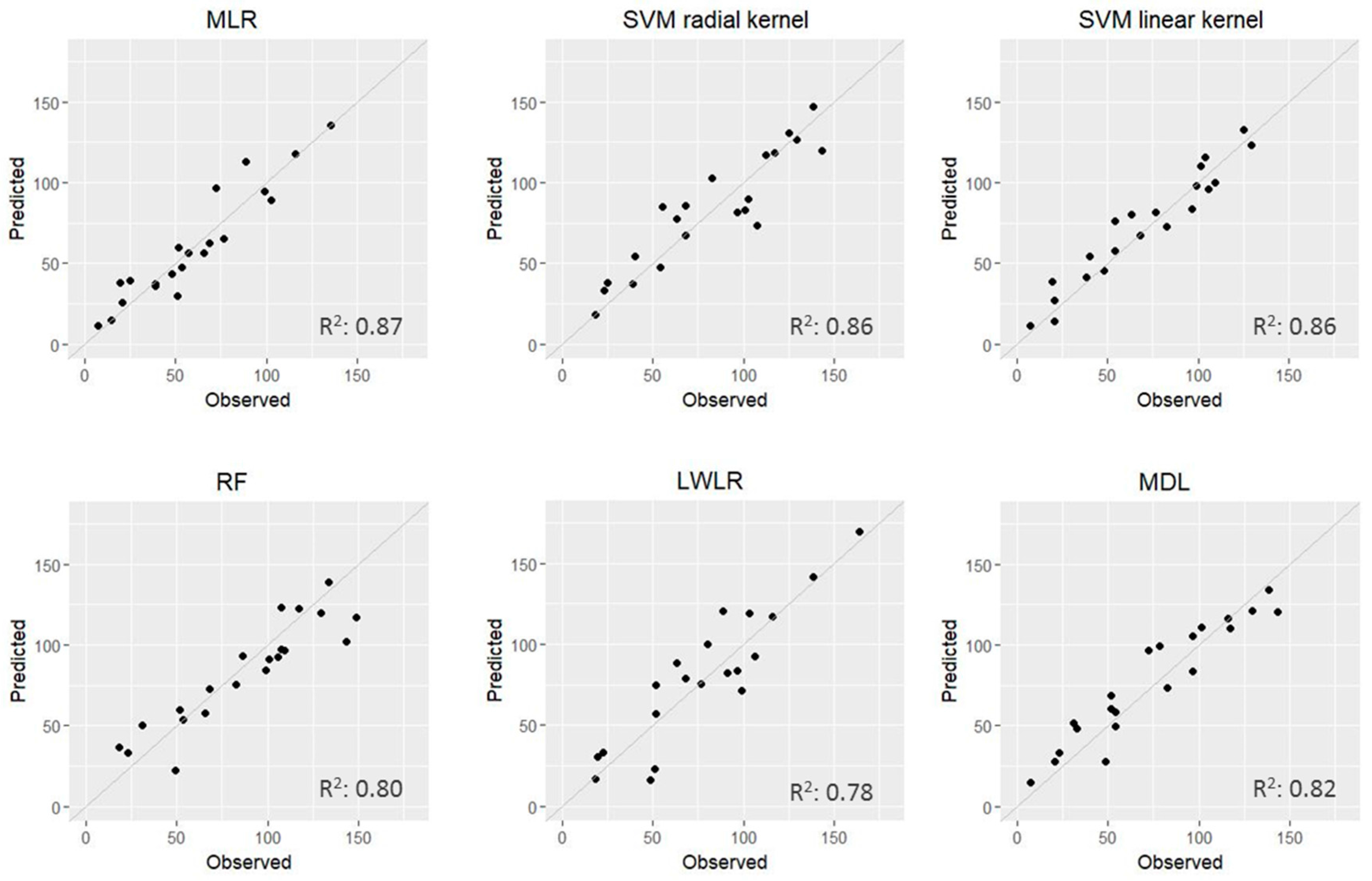
2.7. Model Comparison and Validation

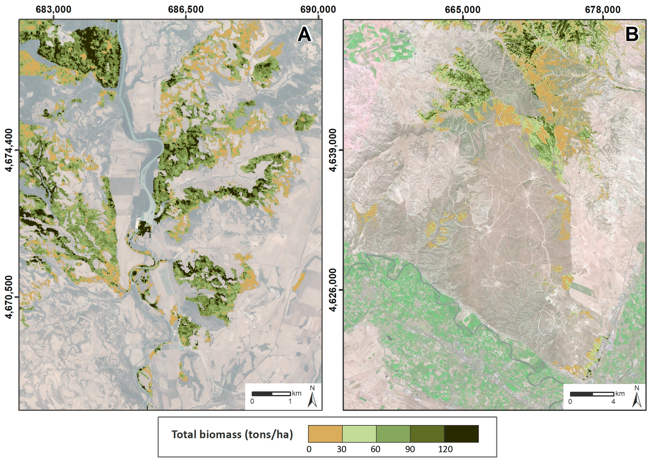
Two types of models were compared: (i) models that include the same independent variables as the MLR one; and (ii) models that use two or three ALS variables, being different from those included in the first comparison.

The original sample was split into a training set of 75% of the cases (62 plots) and a test set of 25% of the cases (21 plots). Validation was performed for all the models, being executed 100 times for those methods with associated randomness as SVM, RF, LWLR, and MDL to increase robustness in the results [34]. In addition, data were normalized in values ranging from 0 to 1 in order to avoid weights saturation according to Görgens [52].

The model performance was compared in terms of root mean square error (RMSE), relative RMSE (%RMSE) and bias. Furthermore, the Friedman nonparametric test was applied using the RMSE of each plot in order to determine differences between models [83]. The Nemenyi post-hoc test was applied to determine whether differences were statistically significant, with a significance level of 0.05 [84]. This test was used only for those cases in which the null-hypothesis of the Friedman test was rejected, implying non-equivalence between models.

3. Results

Table 2. Summary of the field plot characteristics (n = 83). CC is canopy cover; TB is total biomass.

	Min.	Max.	Range	Mean	Standard Deviation
Slope (degrees)	0.70	29.80	29.10	26.10	6.85
Tree height (m)	3.32	16.77	13.44	8.04	2.27
Tree dbh (cm)	8.02	27.54	19.53	16.42	4.11
Tree biomass (tons/ha)	1.27	251.41	250.14	59.58	37.15
Shrub height (m)	0.30	2.06	1.76	1.07	0.44
Shrub CC (%)	1.00	40.00	39.00	11.52	6.09
Shrub biomass (tons/ha)	0.70	47.77	47.07	19.23	12.91
TB (tons/ha)	7.66	253.14	245.48	78.81	42.34

shows a summary of the field plot characteristics. The heights of the inventoried trees range from 3.3 to 16.8 m and they present a variety of diameters, from 8.0 to 27.5 cm. The shrubs present heights ranging from 0.3 to 2.0 m and a CC from 1% to 40%. The average tree biomass fraction is the most important fraction representing almost 75% of TB, and shrub biomass represents in average around 25% of TB.

The ALS metrics selected by the five selection processes are presented in

Table 3. ALS selected metrics using different variable selection methods, when applying a threshold value of 0.2 m to the point cloud data. Seqrep is sequential replacement; P refers to the percentile e.g., P05 is the 5th percentile; Elev. is Elevation; ret. is returns; Elev. AAD is average absolute deviation.

Selection Method		Metrics
		CHM	CHVM	CDM
Spearman’s rank correlation		Elev. mean	Elev. variance	(All ret. above mean)/(Total first ret.) × 100
Stepwise	Backward	Elev. mean	Elev. variance	(All ret. above mean)/(Total first ret.) × 100
	Forward	P20	Elev. variance	% First ret. above mean
	Bidirectional	Elev. mean	Elev. variance	(All ret. above mean)/(Total first ret.) × 100
PCA		P99		% All ret. above 0.2 m
LASSO selection		P40	Elev. standard deviation	% First ret. above 0.2 m
All subsets regression	Seqrep	P05, Elev. mean		% First ret. above mean
	Exhaustive	P25	Elev. variance	% First ret. above mean
	Backward	P90	Elev. AAD	% First ret. above mean
	Forward	P70		% First ret. above mean

. Considering the maximum number of selected variables established, the selection methods included generally one metric related to the canopy height (CHM), one metric associated with the canopy height variability (CHVM), and another expressing the canopy density (CDM). However, sequential replacement all subsets regression, forward all subsets regression, and PCA selected only two metrics.

Regarding CHM, low height percentiles were selected in some cases, but elevation mean and higher percentiles were chosen for the remaining methods. The most selected CHVM was variance. The percentage of first returns above mean and the percentage of all returns above a height break were the CDM metrics with the strongest correlation with TB. All selected metrics showed a logical relation with the dependent variable.

The regression models to estimate TB are summarized in

Table 4. Summary of the models and validation results in terms of RMSE (tons/ha), %RMSE, and bias (tons/ha). SVM r. refers to Support Vector Machine with radial kernel; SVM l. refers to Support Vector Machine with linear kernel; ret. is returns.

		Fitting Phase			Cross-Validation
ALS Metrics	Model	RMSE	%RMSE	Bias	RMSE	%RMSE	Bias	R2
Elev. Variance + P25 + % first ret. above mean	MLR	14.53	18.44	0.00	15.14	19.21	0.01	0.87
	SVM r.	13.94	17.68	−0.36	16.39	20.79	0.00	0.86
	SVM l.	14.56	18.48	−0.74	15.56	19.74	−0.83	0.86
	RF	10.01	12.70	0.59	19.64	24.93	0.75	0.80
	LWLR	12.11	15.37	0.20	19.59	24.86	1.35	0.78
	MDL	14.01	17.77	0.03	17.98	22.81	0.37	0.82
P05 + Elev. mean + % first ret. above mean	SVM r.	13.88	17.61	−0.28	15.50	19.66	−0.26	0.86
Elev. mean + Elev. vriance + (All ret. above mean)/(total first ret. above 0.2 m)	RF	9.64	12.23	0.39	19.14	24.28	0.39	0.80
P40 + Elev. Std.dev + % first ret. above 0.2 m	LWLR	11.38	14.44	−0.45	19.38	24.59	-0.54	0.80

. The MLR and SVM with radial kernel or linear kernel present the lowest RMSE. LWLR, MDL, and RF show lower accuracies. Although most of the models present values of bias close to zero, some of them show a slight overestimation with values close to 1. The selected MLR model including the 25th percentile of height, elevation variance, and the percentage of first returns above mean, present the lowest RMSE with 15.14 tons/ha, a %RMSE of 19.21, and a relative R² after validation of 0.87. SVM with radial kernel including the 5th percentile of height, elevation mean, and percentage of first returns above mean is the second best model. SVM with linear kernel, including the same ALS metrics as the MLR method, presents also similar errors.

Figure 2 shows the independent variables included in the selected MLR model associated with the vertical distribution of ALS returns in three selected field plots representative of the variability of TB of the Aleppo pine forest under study. The TB of smaller pines with low shrub presence (Figure 2A) is lower than in taller pines with higher presence of understory (Figure 2C). Thereby, the TB presents a direct relationship with these variables (Figure 2B). The higher the variance, the higher the TB as the dispersion of the data increases. Similarly, the increase of the percentage of first returns above the mean implies an increase in TB content. The 25th percentile presents an inverse correlation with the TB. A lower value of the 25th percentile implies a higher presence of shrubs in the understory.

Figure 3 presents the scatter plots of observed and predicted TB for the models that include the same variables as the best selected MLR ones. It should be noted that, in this model, logarithmic transformation of the dependent or the independent variables was not required to meet the linear regression assumptions. MLR, SVM with linear kernel and SVM with radial kernel show high coefficients of determination (0.87, 0.86, and 0.86, respectively), while MDL (0.82), RF (0.80), and LWLR (0.78) present slightly lower coefficients of determination, 0.80 and 0.78, respectively. The implementation of the MLR model (Equation (15)) in ArcGIS allowed the estimation of TB.

$$\mathrm{TB}=-14195.1+4753.9\times \mathrm{Elevation} \mathrm{variance}+8992.0\times \mathrm{P}25+699.6\times \% \mathrm{first} \mathrm{returns} \mathrm{above} \mathrm{mean}$$

(15)

The performance comparison between models by using the Friedman test shows that the models are not equivalent with a p-value of 0.00. Thereby, the required application of the post-hoc Nemenyi test indicates that no statistically significant differences exist between models, with 95% of probability.

Figure 4 shows the TB mapping for the study area. The north part of the study area (Figure 4A) shows a heterogeneous Aleppo pine forest with higher TB values (above 150 tons/ha), which denote mature forested areas with the presence of shrubs and taller trees. In contrast, the southern part (Figure 4B) shows some homogeneous areas with lower TB values (bellow 10 tons/ha). These areas have been affected more recently by several wildfires, contrasting with the pines of area A or some north stands of area B that have higher ages, presenting TB values ranging from approximately 30 tons/ha to more than 120 tons/ha.

4. Discussion

The results demonstrate that low density ALS data can be used to accurately estimate TB. Regarding the selection method, all subsets regression and selection based on Spearman’s rank was the most powerful technique for ALS metrics selection. LASSO selection was also a good technique. However, the use of Stepwise selection and PCA showed a restricted power in identifying the best subsets. These findings agree with Garcia-Gutierrez et al. [48], who found that Stepwise selection was the technique with less power, but all subsets regression obtained good results. Although PCA was used by Silva et al. [49] for stem volume modeling, it has been outperformed by other selection techniques for TB estimation.

The selection of a reduced number of biologically representative variables increases the understanding of models for forest management purposes. In this sense, the use of automatic methods for variable selection is considerably less time-demanding when modeling. The three ALS-derived variables included in the best model were coherent and analogous to those derived for characterizing forest vertical diversity [22] and aboveground biomass [15,36]. Variables derived from digital surface models (DSM) were not computed in this study. Nevertheless, they have been proposed in other studies because they seem more suitable for tree damage detection [29] or estimation of vertical diversity [19] when not using an area based approach (ABA).These variables concern the variability of different strata of the point cloud and canopy cover distribution.

The comparison between regression models shows that the MLR model had the lowest RMSE (15.14 tons/ha) and bias (0.01), matching with the values obtained by other authors for aboveground biomass estimation [73,85]. Thus, according to Görgens et al. [52] and Domingo et al. [38], MLR slightly outperforms other nonparametric methods. Although MLR was the best model, no statistically significant differences were found with other methods. These results partly agree with other approaches [34,36,48], which obtained lower estimation errors with nonparametric techniques. The use of selection methods is useful to better determine the best subset of variables and the comparison of models, such as MLR, SVM with radial kernel, SVM with linear kernel, and LWLR.

TB estimation by using trees and shrub allometric equations and low-density ALS data is considered to better account for biomass and carbon reservoirs in Mediterranean forest ecosystems. The comparison of different models for TB estimation including other tree species or biomass estimation in shrubland areas may be considered. In this sense, 35% of the forested land in Spain, which includes grasslands, shrubland, and trees, is covered by shrubs [83]. Furthermore, shrub species in the understory, with an average presence of 24%, constitute an important part of TB in Mediterranean Aleppo pine forest. This pattern is also common in the understory of other Mediterranean forests as for example Pinus and Quercus ilex. Shrubland areas are also especially important due to the abandonment of crops and wildfire disturbances [13], that might even increase the presence of these species in the near future. Consequently, further research is needed on the estimation of TB using tree and shrub allometric equations and low density ALS data in shrubland and burned areas to compare with previous higher point density studies. Moreover, the use of ALS technology with higher density, the use of terrestrial LiDAR, or the fusion with high spatial resolution images derived by unmanned aerial vehicles might be useful to better account for forest biomass.

5. Conclusions

Allometric equations are one of the available methods for estimating forest structural parameters. This method has been widely applied to accurately estimate tree height, crown diameter, basal area, stem density, volume or aboveground biomass at plot level and to relate it to ALS data to estimate it at stand level [36,47,56,57,86]. Nevertheless, little research has focused on the estimation of biomass with ALS data including shrub fraction. The lack of knowledge of shrub vegetation associated with the traditionally necessary destructive sampling to generate forest structure equations might have been one of the drawbacks of including those species for biomass and carbon account. In this sense, the development of new allometric equations for shrub species, defined to estimate biomass from simple field measurements and the generalization of ALS data have opened new opportunities for TB estimation.

This study assesses the usefulness of low point density ALS data to accurately estimate biomass, including tree and shrub fraction, in an Aleppo pine forest. The comparison of the effectiveness of five variable selection methods increased modeling efficiency. All subsets regression and manual selection based on Spearman’s rank were the most powerful techniques. LASSO selection was also a good technique but, Stepwise selection and PCA showed less power to identify the best subsets. The comparison of parametric and nonparametric regression methods showed that the best model for TB estimation was the MLR. This model included three ALS metrics: the 25th percentile of the return heights, the variance, and the percentage of first returns above the mean, presenting an RMSE of 15.14 tons/ha and a bias of 0.01. No statistically significant differences between the generated models were found. The results allow TB mapping at the regional scale providing useful information for forest management purposes, with values ranging from below 10 tons/ha to areas above 150 tons/ha. This study moves a step forward to compute TB by using allometric tree and shrub equations and ALS data to better account for forest biomass as assets to manage greenhouse gases from a local to a global scale.

References

1. Martinuzzi, S.; Vierling, L.A.; Gould, W.A.; Falkowski, M.J.; Evans, J.S.; Hudak, A.T.; Vierling, K.T. Mapping snags and understory shrubs for LiDAR based assessment of wildlife habitat suitability. Remote Sens. Environ. 2009, 113, 2533–2546. [Google Scholar] [CrossRef]
2. Wing, B.M.; Ritchie, M.W.; Boston, K.; Cohen, W.B.; Gitelman, A.; Olsen, M.J. Prediction of understory vegetation cover with airborne LiDAR in an interior ponderosa pine forest. Remote Sens. Environ. 2012, 124, 730–741. [Google Scholar] [CrossRef]
3. Lal, R. Sequestration of atmospheric CO2 in global carbon pools. Energy Environ. Sci. 2008, 1, 86–100. [Google Scholar] [CrossRef]
4. Pan, Y.; Birdsey, R.A.; Fang, J.; Houghton, R.; Kauppi, P.E.; Kurz, W.A.; Phillips, O.L.; Shvidenko, A.; Lewis, S.L.; Canadell, J.G.; et al. A large and persistent carbon sink in the world’s forests. Science 2011, 333, 988–993. [Google Scholar] [CrossRef] [PubMed]
5. Hoen, H.F.; Solberg, B. Potential and Economic Efficiency of Carbon Sequestration in Forest Biomass through Silvicultural Management. For. Sci. 1994, 40, 429–451. [Google Scholar]
6. Gren, I.-M.; Aklilu, A.Z. Policy design for forest carbon sequestration: A review of the literature. For. Policy Econ. 2016, 70, 128–136. [Google Scholar] [CrossRef]
7. Seiler, W.; Crutzen, P.J. Estimates of gross and net fluxes of carbon between the biosphere and the atmosphere from biomass burning. Clim. Chang. 1980, 2, 207–247. [Google Scholar] [CrossRef]
8. Andreae, M.O.; Browell, E.V.; Garstang, M.; Gregory, G.L.; Harriss, R.C.; Hill, G.F.; Jacob, D.J.; Pereira, M.C.; Sachse, G.W.; Setzer, A.W.; et al. Biomass-burning emissions and associated haze layers over Amazonia. J. Geophys. Res. 1988, 93, 1509–1527. [Google Scholar] [CrossRef]
9. Van der Werf, G.R.; Randerson, J.T.; Giglio, L.; Collatz, G.J.; Mu, M.; Kasibhatla, P.S.; Morton, D.C.; DeFries, R.S.; Jin, Y.; van Leeuwen, T.T. Global fire emissions and the contribution of deforestation, savanna, forest, agricultural, and peat fires (1997–2009). Atmos. Chem. Phys. 2010, 10, 11707–11735. [Google Scholar] [CrossRef] [Green Version]
10. Akagi, S.K.; Yokelson, R.J.; Burling, I.R.; Meinardi, S.; Simpson, I.; Blake, D.R.; McMeeking, G.R.; Sullivan, A.; Lee, T.; Kreidenweis, S.; et al. Measurements of reactive trace gases and variable O3 formation rates in some South Carolina biomass burning plumes. Atmos. Chem. Phys. 2013, 13, 1141–1165. [Google Scholar] [CrossRef]
11. Wiedinmyer, C.; Akagi, S.K.; Yokelson, R.J.; Emmons, L.K.; Al-Saadi, J.A.; Orlando, J.J.; Soja, A.J. The Fire INventory from NCAR (FINN): A high resolution global model to estimate the emissions from open burning. Geosci. Model Dev. 2011, 4, 625–641. [Google Scholar] [CrossRef]
12. Penman, J.; Gytarsky, M.; Hiraishi, T.; Krug, T.; Kruger, D.; Pipatti, R.; Buendia, L.; Miwa, K.; Ngara, T.; Tanabe, K.; et al. Good Practice Guidance for Land Use, Land-Use Change and Forestry; Intergovernmental Panel on Climate Change (IPCC); IGES: Hayama, Japan, 2003. [Google Scholar]
13. Pasalodos-Tato, M.; Ruiz-Peinado, R.; del Río, M.; Montero, G. Shrub biomass accumulation and growth rate models to quantify carbon stocks and fluxes for the Mediterranean region. Eur. J. For. Res. 2015, 134, 537–553. [Google Scholar] [CrossRef]
14. García, M.; Riaño, D.; Chuvieco, E.; Danson, F.M. Estimating biomass carbon stocks for a Mediterranean forest in central Spain using LiDAR height and intensity data. Remote Sens. Environ. 2010, 114, 816–830. [Google Scholar] [CrossRef]
15. Montealegre-Gracia, A.L.; Lamelas-Gracia, M.T.; García-Martín, A.; de la Riva-Fernández, J.; Escribano-Bernal, F. Using low-density discrete Airborne Laser Scanning data to assess the potential carbon dioxide emission in case of a fire event in a Mediterranean pine forest. GISci. Remote Sens. 2017, 54, 721–740. [Google Scholar] [CrossRef]
16. Latifi, H.; Nothdurft, A.; Koch, B. Non-parametric prediction and mapping of standing timber volume and biomass in a temperate forest: Application of multiple optical/LiDAR-derived predictors. Forestry 2010, 83, 395–407. [Google Scholar] [CrossRef]
17. Vosselman, G.; Maas, H.G. Airborne and Terrestrial Laser Scanning; Whittles Publishing: Scotland, UK, 2010; ISBN 978-1904445-87-6. [Google Scholar]
18. Maltamo, M.; Næsset, E.; Vauhkonen, J. Eds. Forestry Applications of Airborne Laser Scanning: Concepts and Case Studies; Springer: Dordrecht, The Netherlands, 2014; Volume 27, ISBN 978-94-017-8662-1. [Google Scholar]
19. Kane, V.R.; Lutz, J.A.; Roberts, S.L.; Smith, D.F.; McGaughey, R.J.; Povak, N.A.; Brooks, M.L. Landscape-scale effects of fire severity on mixed-conifer and red fir forest structure in Yosemite National Park. For. Ecol. Manag. 2013, 287, 17–31. [Google Scholar] [CrossRef]
20. Kane, V.R.; North, M.P.; Lutz, J.A.; Churchill, D.J.; Roberts, S.L.; Smith, D.F.; McGaughey, R.J.; Kane, J.T.; Brooks, M.L. Assessing fire effects on forest spatial structure using a fusion of Landsat and airborne LiDAR data in Yosemite National Park. Remote Sens. Environ. 2014, 151, 89–101. [Google Scholar] [CrossRef]
21. Listopad, C.M.C.S.; Masters, R.E.; Drake, J.; Weishampel, J.; Branquinho, C. Structural diversity indices based on airborne LiDAR as ecological indicators for managing highly dynamic landscapes. Ecol. Indic. 2015, 57, 268–279. [Google Scholar] [CrossRef]
22. Bottalico, F.; Chirici, G.; Giannini, R.; Mele, S.; Mura, M.; Puxeddu, M.; Mcroberts, R.E.; Valbuena, R.; Travaglini, D. Modeling Mediterranean forest structure using airborne laser scanning data. Int. J. Appl. Earth Obs. Geoinf. 2017, 57, 145–153. [Google Scholar] [CrossRef]
23. García, M.; Riaño, D.; Chuvieco, E.; Salas, J.; Danson, F.M. Multispectral and LiDAR data fusion for fuel type mapping using Support Vector Machine and decision rules. Remote Sens. Environ. 2011, 115, 1369–1379. [Google Scholar] [CrossRef]
24. Rosa, M.F.; Stow, D.A. Mapping fuels at the wildland-urban interface using colour ortho-images and LiDAR data. Geocarto Int. 2014, 29, 570–588. [Google Scholar] [CrossRef]
25. Hall, S.A.; Burke, I.C.; Box, D.O.; Kaufmann, M.R.; Stoker, J.M. Estimating stand structure using discrete-return lidar: An example from low density, fire prone ponderosa pine forests. For. Ecol. Manag. 2005, 208, 189–209. [Google Scholar] [CrossRef]
26. Riaño, D.; Meier, E.; Allgöwer, B.; Chuvieco, E.; Ustin, S.L. Modeling airborne laser scanning data for the spatial generation of critical forest parameters in fire behavior modeling. Remote Sens. Environ. 2003, 86, 177–186. [Google Scholar] [CrossRef]
27. Ranson, K.J.; Sun, G.; Kovacs, K.; Kharuk, V.I. Use of ICESat GLAS data for forest disturbance studies in central Siberia. In Proceedings of the IEEE International Geoscience and Remote Sensing Symposium, Anchorage, AK, USA, 20–24 September 2004; Volume 3, pp. 1936–1939. [Google Scholar] [CrossRef]
28. Honkavaara, E.; Litkey, P.; Nurminen, K. Automatic Storm Damage Detection in Forests Using High-Altitude Photogrammetric Imagery. Remote Sens. 2013, 5, 1405–1424. [Google Scholar] [CrossRef]
29. Rahman, M.T.; Rashed, T. Urban tree damage estimation using airborne laser scanner data and geographic information systems: An example from 2007 Oklahoma ice storm. Urban For. Urban Green. 2015, 14, 562–572. [Google Scholar] [CrossRef]
30. Estornell, J.; Ruiz, L.A.; Velázquez-Martí, B.; Hermosilla, T. Analysis of the factors affecting LiDAR DTM accuracy in a steep shrub area. Int. J. Digit. Earth 2011, 4, 521–538. [Google Scholar] [CrossRef]
31. Estornell, J.; Ruiz, L.A.; Velázquez-Martí, B.; Hermosilla, T. Estimation of biomass and volume of shrub vegetation using LiDAR and spectral data in a Mediterranean environment. Biomass Bioenergy 2012, 46, 710–721. [Google Scholar] [CrossRef]
32. Greaves, H.E.; Vierling, L.A.; Eitel, J.U.H.; Boelman, N.T.; Magney, T.S.; Prager, C.M.; Griffin, K.L. High-resolution mapping of aboveground shrub biomass in Arctic tundra using airborne lidar and imagery. Remote Sens. Environ. 2016, 184, 361–373. [Google Scholar] [CrossRef]
33. Li, A.; Dhakal, S.; Glenn, N.; Spaete, L.; Shinneman, D.; Pilliod, D.; Arkle, R.; McIlroy, S. Lidar Aboveground Vegetation Biomass Estimates in Shrublands: Prediction, Uncertainties and Application to Coarser Scales. Remote Sens. 2017, 9, 903. [Google Scholar] [CrossRef]
34. García-Gutiérrez, J.; Martínez-Álvarez, F.; Troncoso, A.; Riquelme, J.C. A comparison of machine learning regression techniques for LiDAR-derived estimation of forest variables. Neurocomputing 2015, 167, 24–31. [Google Scholar] [CrossRef]
35. Shendryk, I.; Hellström, M.; Klemedtsson, L.; Kljun, N. Low-Density LiDAR and Optical Imagery for Biomass Estimation over Boreal Forest in Sweden. Forests 2014, 5, 992–1010. [Google Scholar] [CrossRef]
36. Guerra-Hernández, J.; Görgens, E.B.; García-Gutiérrez, J.; Carlos, L.; Rodriguez, E.; Tomé, M.; González-Ferreiro, E. European Journal of Remote Sensing Comparison of ALS based models for estimating aboveground biomass in three types of Mediterranean forest. Eur. J. Remote Sens. 2016, 49, 185–204. [Google Scholar] [CrossRef]
37. Montagnoli, A.; Fusco, S.; Terzaghi, M.; Kirschbaum, A.; Pflugmacher, D.; Cohen, W.B.; Scippa, G.S.; Chiatante, D. Estimating forest aboveground biomass by low density lidar data in mixed broad-leaved forests in the Italian Pre-Alps. For. Ecosyst. 2015, 2. [Google Scholar] [CrossRef]
38. Domingo, D.; Lamelas-Gracia, M.T.; Montealegre-Gracia, A.L.; de la Riva-Fernández, J. Comparison of regression models to estimate biomass losses and CO2 emissions using low-density airborne laser scanning data in a burnt Aleppo pine forest. Eur. J. Remote Sens. 2017, 50, 384–396. [Google Scholar] [CrossRef]
39. Gaveau, D.L.A.; Hill, R.A. Quantifying canopy height underestimation by laser pulse penetration in small-footprint airborne laser scanning data. Can. J. Remote Sens. 2003, 29, 650–657. [Google Scholar] [CrossRef]
40. Hill, R.A.; Thomson, A.G. Mapping woodland species composition and structure using airborne spectral and LiDAR data. Int. J. Remote Sens. 2005, 26, 3763–3779. [Google Scholar] [CrossRef]
41. Hopkinson, C.; Chasmer, L.E.; Sass, G.; Creed, I.F.; Sitar, M.; Kalbfleisch, W.; Treitz, P. Vegetation class dependent errors in lidar ground elevation and canopy height estimates in a boreal wetland environment. Can. J. Remote Sens. 2005, 31, 191–206. [Google Scholar] [CrossRef]
42. Riaño, D.; Chuvieco, E.; Ustin, S.L.; Salas, J.; Rodríguez-Pérez, J.R.; Ribeiro, L.M.; Viegas, D.X.; Moreno, J.M.; Fernández, H. Estimation of shrub height for fuel-type mapping combining airborne LiDAR and simultaneous color infrared ortho imaging. Int. J. Wildl. Fire 2007, 16, 341. [Google Scholar] [CrossRef]
43. Meng, X.; Currit, N.; Zhao, K. Ground Filtering Algorithms for Airborne LiDAR Data: A Review of Critical Issues. Remote Sens. 2010, 2, 833–860. [Google Scholar] [CrossRef]
44. Loudermilk, E.L.; Hiers, J.K.; O’Brien, J.J.; Mitchell, R.J.; Singhania, A.; Fernandez, J.C.; Cropper, W.P.; Slatton, K.C. Ground-based LIDAR: A novel approach to quantify fine-scale fuelbed characteristics. Int. J. Wildl. Fire 2009, 18, 676. [Google Scholar] [CrossRef]
45. Velázquez-Martí, B.; Fernández-González, E.; Estornell, J.; Ruiz, L.A. Dendrometric and dasometric analysis of the bushy biomass in Mediterranean forests. For. Ecol. Manag. 2010, 259, 875–882. [Google Scholar] [CrossRef]
46. González, G.M.; Pasalodos-Tato, M.; López-Senespleda, E.; Onrubia, R.; Bravo-Oviedo, A.; Ruiz-Peinado, R. Contenido de Carbono en la biomasa de las principales especies de matorral y arbustedos de España. In Proceedings of the 6th Congreso Forestal Español, Pontevedra, Spain, 10 June–14 June 2013; Sociedad Española de Ciencias Forestales: Pontevedra, Spain, 2013. [Google Scholar]
47. Montealegre, A.L.; Lamelas, M.T.; de la Riva, J.; García-Martín, A.; Escribano, F. Use of low point density ALS data to estimate stand-level structural variables in Mediterranean Aleppo pine forest. Forestry 2016, 89, 373–382. [Google Scholar] [CrossRef]
48. Garcia-Gutierrez, J.; Gonzalez-Ferreiro, E.; Riquelme-Santos, J.C.; Miranda, D.; Dieguez-Aranda, U.; Navarro-Cerrillo, R.M. Evolutionary feature selection to estimate forest stand variables using LiDAR. Int. J. Appl. Earth Obs. Geoinf. 2014, 26, 119–131. [Google Scholar] [CrossRef]
49. Silva, C.A.; Klauberg, C.; Hudak, A.T.; Vierling, L.A.; Liesenberg, V.; Carvalho, S.P.C.E.; Rodriguez, L.C.E. A principal component approach for predicting the stem volume in Eucalyptus plantations in Brazil using airborne LiDAR data. Forestry 2016, 89, 422–433. [Google Scholar] [CrossRef]
50. Gagliasso, D.; Hummel, S.; Temesgen, H. A Comparison of Selected Parametric and Non-Parametric Imputation Methods for Estimating Forest Biomass and Basal Area. Open J. For. 2014, 4, 42–48. [Google Scholar] [CrossRef]
51. Gleason, C.J.; Im, J. Forest biomass estimation from airborne LiDAR data using machine learning approaches. Remote Sens. Environ. 2012, 125, 80–91. [Google Scholar] [CrossRef]
52. Görgens, E.B.; Montaghi, A.; Rodriguez, L.C.E. A performance comparison of machine learning methods to estimate the fast-growing forest plantation yield based on laser scanning metrics. Comput. Electron. Agric. 2015, 116, 221–227. [Google Scholar] [CrossRef]
53. Cuadrat, J.M.; Saz, M.A.; Vicente-Serrano, S.M. Atlas Climático de Aragón; Gobierno de Aragón: Aragón, Spain, 2007. [Google Scholar]
54. Plan Nacional de Ortofotografía Aérea LiDAR. Available online: http://pnoa.ign.es/presentacion (accessed on 16 January 2018).
55. Hair, J.F.; Prentice, E.; Cano, D. Análisis Multivariante; Prentice-Hall: Madrid, Spain, 1999; ISBN 9788483220351. [Google Scholar]
56. Næsset, E. Predicting forest stand characteristics with airborne scanning laser using a practical two-stage procedure and field data. Remote Sens. Environ. 2002, 80, 88–99. [Google Scholar] [CrossRef]
57. Næsset, E.; Økland, T. Estimating tree height and tree crown properties using airborne scanning laser in a boreal nature reserve. Remote Sens. Environ. 2002, 79, 105–115. [Google Scholar] [CrossRef]
58. Ruiz-Peinado, R.; Del Rio, M.; Montero, G. New models for estimating the carbon sink capacity of Spanish softwood species. For. Syst. 2011, 20, 176. [Google Scholar] [CrossRef]
59. MAGRAMA Mapa Forestal de España 1:50.000 (MFE50). Available online: http://www.magrama.gob.es/es/biodiversidad/servicios/banco-datos-naturaleza/informacion-disponible/mfe50.aspx (accessed on 4 May 2016).
60. Montealegre, A.L.; Lamelas, M.T.; de la Riva, J. Interpolation Routines Assessment in ALS-Derived Digital Elevation Models for Forestry Applications. Remote Sens. 2015, 7, 8631–8654. [Google Scholar] [CrossRef]
61. Evans, J.S.; Hudak, A.T. A Multiscale Curvature Algorithm for Classifying Discrete Return LiDAR in Forested Environments. IEEE Trans. Geosci. Remote Sens. 2007, 45, 1029–1038. [Google Scholar] [CrossRef]
62. Evans, J.S.; Hudak, A.T.; Faux, R.; Smith, A.M.S. Discrete Return Lidar in Natural Resources: Recommendations for Project Planning, Data Processing, and Deliverables. Remote Sens. 2009, 1, 776–794. [Google Scholar] [CrossRef]
63. FUSION Version Check. Available online: http://forsys.sefs.uw.edu/fusion/fusionlatest.html (accessed on 16 January 2018).
64. Nilsson, M. Estimation of tree heights and stand volume using an airborne lidar system. Remote Sens. Environ. 1996, 56, 1–7. [Google Scholar] [CrossRef]
65. Kaiser, H.F. The Application of Electronic Computers to Factor Analysis. Educ. Psychol. Meas. 1960, 20, 141–151. [Google Scholar] [CrossRef]
66. Horst, P. Factor Analysis of Data Matrices, 1st ed.; Holt, Rinehart and Winston: New York, NY, USA, 1965. [Google Scholar] [CrossRef]
67. Kaiser, H.F. The varimax criterion for analytic rotation in factor analysis. Psychometrika 1958, 23, 187–200. [Google Scholar] [CrossRef]
68. Tibshirani, R. Regression shrinkage and selection via the lasso: A retrospective. J. R. Stat. Soc. Ser. B (Stat. Methodol.) 2011, 73, 273–282. [Google Scholar] [CrossRef]
69. Miller, A.J. Subset Selection in Regression; Chapman & Hall/CRC: Boca Raton, FL, USA, 2002; ISBN 9781584881711. [Google Scholar]
70. Hermosilla, T.; Ruiz, L.A.; Kazakova, A.N.; Coops, N.C.; Moskal, L.M. Estimation of forest structure and canopy fuel parameters from small-footprint full-waveform LiDAR data. Int. J. Wildl. Fire 2014, 23, 224. [Google Scholar] [CrossRef]
71. Means, J.; Acker, S.; Harding, D.; Blair, J.; Lefsky, M.; Cohen, W.; Harmon, M.; McKee, W. Use of large-footprint scanning airborne lidar to estimate forest stand characteristics in the western Cascades of Oregon. Remote Sens. Environ. 1999, 67, 298–308. [Google Scholar] [CrossRef]
72. Lim, K.; Treitz, P.; Wulder, M.; St-Onge, B.; Flood, M. LiDAR remote sensing of forest structure. Prog. Phys. Geogr. 2003, 27, 88–106. [Google Scholar] [CrossRef]
73. Gonzalez-Ferreiro, E.; Dieguez-Aranda, U.; Miranda, D. Estimation of stand variables in Pinus radiata D. Don plantations using different LiDAR pulse densities. Forestry 2012, 85, 281–292. [Google Scholar] [CrossRef]
74. García, D.; Godino, M.; Mauro, F. Lidar: Aplicación Práctica Al Inventario Forestal; Académica Española: ‎Madrid, Spain, 2012; ISBN 3659009555. [Google Scholar]
75. Watt, M.S.; Meredith, A.; Watt, P.; Gunn, A.; Andersen, H.; Reutebuch, S.; Nelson, R. Use of LiDAR to estimate stand characteristics for thinning operations in young Douglas-fir plantations. N. Z. J. For. Sci. 2013, 43, 1–10. [Google Scholar] [CrossRef]
76. González-Olabarria, J.-R.; Rodríguez, F.; Fernández-Landa, A.; Mola-Yudego, B. Mapping fire risk in the Model Forest of Urbión (Spain) based on airborne LiDAR measurements. For. Ecol. Manag. 2012, 282, 149–156. [Google Scholar] [CrossRef]
77. Mountrakis, G.; Im, J.; Ogole, C. Support vector machines in remote sensing: A review. ISPRS J. Photogramm. Remote Sens. 2011, 66, 247–259. [Google Scholar] [CrossRef]
78. Breiman, L. Random Forest. Mach. Learn. 2001, 45, 5–32. [Google Scholar] [CrossRef]
79. Liaw, A.; Wiener, M. Classification and Regression by randomForest. R News 2002, 2, 18–22. [Google Scholar]
80. Van Essen, D.C.; Drury, H.A.; Dickson, J.; Harwell, J.; Hanlon, D.; Anderson, C.H. An integrated software suite for surface-based analyses of cerebral cortex. J. Am. Med. Inform. Assoc. 2001, 8, 443–459. [Google Scholar] [CrossRef] [PubMed]
81. Cleveland, W.S.; Devlin, S.J. Locally Weighted Regression: An Approach to Regression Analysis by Local Fitting. J. Am. Stat. Assoc. 1988, 83, 596–610. [Google Scholar] [CrossRef]
82. Rissanen, J. Modeling by shortest data description. Automatica 1978, 14, 465–471. [Google Scholar] [CrossRef]
83. Stojanova, D.; Panov, P.; Gjorgjioski, V.; Kobler, A.; Džeroski, S. Estimating vegetation height and canopy cover from remotely sensed data with machine learning. Ecol. Inform. 2010, 5, 256–266. [Google Scholar] [CrossRef]
84. Nemenyi, P. Distribution-Free Multiple Comparisons. Ph.D. Thesis, Princeton University, Princenton, NY, USA, 1963. [Google Scholar]
85. Montealegre, A.L.; Lamelas, M.T.; de la Riva, J.; García-Martín, A.; Escribano, F. Assessment of Biomass and Carbon Content in a Mediterranean Aleppo Pine Forest Using ALS Data. In Proceedings of the 1st International Electronic Conference on Remote Sensing, Basel, Switzerland, 22 June–5 July 2005; MDPI: Basel, Switzerland, 2015; Volume 1, p. d004. [Google Scholar]
86. Popescu, S.C.; Wynne, R.H.; Nelson, R.F. Measuring individual tree crown diameter with lidar and assessing its influence on estimating forest volume and biomass. Can. J. Remote Sens. 2003, 29, 564–577. [Google Scholar] [CrossRef]
Figure 1. Study area. Land cover types and location of 83 forest inventory plots. High spatial resolution orthophotography of the Spanish National Plan for Aerial Orthophotography [54] is used as backdrop. Coordinate System: ETRS89 UTM Zone 30 N.
Forests 09 00158 g001
Figure 2. Airborne Laser Scanning (ALS) metrics associated with the vertical distribution of point cloud returns in three selected field plots representative of the study area: (A) smaller pines with low presence of shrubs (area B); (B) average height pines with an intermediate presence of understory (area A); (C) taller pines with high presence of shrubs (area A). The red square represents the average of the shrub height in each plot.
Forests 09 00158 g002
Figure 3. Scatterplot of predicted vs. observed values of total biomass (TB) (tons/ha) using different regression methods.
Forests 09 00158 g003
Figure 4. Maps of TB. High spatial resolution orthophotography from Spanish National Plan for Aerial Orthophotography (PNOA) [54] is used as backdrop. Coordinate System: ETRS89 UTM Zone 30 N.
Forests 09 00158 g004