Assessing Ecosystem Services from the Forestry-Based Reclamation of Surface Mined Areas in the North Fork of the Kentucky River Watershed


1
Department of Forestry and Natural Resources, TP Cooper Building, University of Kentucky, Lexington, KY 40546, USA
2
CAS Key Laboratory of Forest Ecology and Management, Institute of Applied Ecology, Chinese Academy of Sciences, Shenyang 110016, China
*
Author to whom correspondence should be addressed.
Forests 2018, 9(10), 652; https://doi.org/10.3390/f9100652
Submission received: 31 August 2018
/
Revised: 1 October 2018
/
Accepted: 16 October 2018
/
Published: 19 October 2018
(This article belongs to the Special Issue Forest Landscape Ecology: Linking Past, Present, and Future Data)
Abstract
:Surface mining is a major driver of land use land cover (LULC) change in many mountainous areas such as the Appalachian region. Typical reclamation practices often result in land cover dominated by grass and shrubs. Assessing ecosystem services that can be obtained from a forest landscape may help policy-makers and other stakeholders fully understand the benefits of forestry-based reclamation (FRA). The objectives of this study are to (1) identify how surface mining and reclamation changed the LULC of a watershed encompassing the north fork of the Kentucky River, (2) assess the biophysical value of four major ecosystem services under the contemporary LULC condition, and (3) assess the benefits of the FRA scenario in the provision of ecosystem services. Geographic Information System (GIS) was used to study the LULC change and InVEST software models for ecosystem services assessment. The results indicate that watershed’s forest area has decreased by 7751 hectares from 2001 to 2011 and mining/reclamation activities may have contributed 65% of the overall changes in LULC. Barren and grassland land covers provide less carbon storage, yield more water, and export more sediments and nutrients than forests. At the watershed level, the FRA scenario increased carbon storage (13%) and reduced water yield (5%), sediment export (40%), and nutrient export (7%). The provision of these ecosystem services varies at the subwatershed level, and such spatial heterogeneity is primarily driven by land cover composition, precipitation, and topography. This study provides critical information regarding the ecological benefits of restoring mined land to assist policy and decision making at landscape scales.
1. Introduction
Land cover and land use (LULC) change is a major force of global environmental change [1], with as much as 50% of the earth’s ice-free land surface having been transformed as a direct consequence of land uses [2,3]. The changes of LULC help humans extract natural resources to meet society’s growing needs of food, fiber, water, and shelter, but often at the expense of degrading environmental conditions [4,5], such as alteration of the climate system and atmospheric composition [6], land degradation [7,8], changes in hydrology [9], and loss of biodiversity [4]. Understanding the pattern of LULC change and its impacts for human well-being is a key in land change science as a coupled system of human and environment [3]. Although studying the cause and consequences of LULC change can be conducted at any spatial scales, it has been increasingly recognized that landscapes represent a pivotal scale domain for the research of LULC change because landscape scales are more directly linked with the land management, environmental policy, and application of sustainability [10].
Among all LULC change types, few are as intensive as surface mining, which extracts minerals near the Earth’s surface [11,12]. Surface coal mining generally involves a sequence of operations including vegetation clearing, topsoil removal, drilling, and blasting the hard strata over the coal seam, and then the subsequent extracting and transporting of coals [11,13]. It has been predominantly conducted in the central Appalachian Mountains of the US that are mainly located in southern West Virginia, eastern Kentucky, southwestern Virginia, and northeastern Tennessee [14]. Various studies have documented persistent negative impacts of mining on ecological integrity of Appalachia [14,15,16]. One of the most prominent environmental impacts is the degradation of water quality in Appalachia as the overburden from surface mining has buried more than 2000 km of stream channels [15] and permanently altered drainage networks and topography [17,18]. Forest clearing, soil loss, and subsequent substrate compaction induced by reclamation further contribute to water quality deterioration and the increased flood risk in downstream communities [16,17]. Surface mining can also convert an area that was a carbon sink into a carbon source through the depletion of forest carbon storage and the burning of coal in electric power plants [14,19].
The Surface Mining Control and Reclamation Act of 1977 (SMCRA) was initiated to mitigate the negative environmental effects of coal mining in the United States of America. SMCRA requires reclamation of mountaintop-mined sites to a state that provides an equal or better use than the pre-mining condition. However, the law is vague on what constitutes equal or better use. Often the reclamation approach has resulted in plant communities dominated by persistent herbaceous species, grasses sown during reclamation, and early successional woody species [20], which is not an adequate substitute for the original diverse forest [21]. To address this issue, the Appalachian Regional Reforestation Initiative (ARRI) was formed in 2004 by a coalition of citizens, government officials, and coal industry representatives dedicated to restoring forests in the abandoned coal mines [20,22,23]. ARRI advocates a technique known as the Forestry Reclamation Approach, or FRA, a series of recommendations to guide successful regeneration of native forest on surface mined sites [24]. The five-step guideline of FRA includes: creating a suitable growth medium, grading the top soil to get a noncompacted growth medium, planting less competitive ground covers that are compatible with trees, planting a mix of early successional woody species for wildlife and soil stability and commercially valuable crops, and using proper tree planting techniques to accommodate the seedling’s root system [20,23]. Experimental reclamation trials utilizing FRA techniques have been successful in Kentucky [24] and West Virginia [25]. However, the reclamation approach is not in widespread use in the Appalachian region because its implementation is difficult and expensive for mining companies [23]. In addition, local residents and the public are nonchalant toward forestry-based reclamation practices. Such situations might have arisen because the value of ecosystem services from forests in this landscape are not adequately valued. The public, mining companies, and policy-makers are not fully aware of the extent of ecosystem degradation induced by surface mining and the benefits to human wellbeing brought by the FRA approach compared to traditional reclamation practices.
Ecosystem services evaluation can help the decision making and the implementation of FRA techniques in reestablishing forest patches in the Appalachian Mountains. Evaluation of ecosystem services such as carbon storage, flood control, sediment, and nutrient retention at a local watershed or regional level can help establish sound ecological restoration policies [26] because it can help individuals and stakeholders appreciate and capture the value of ecosystem services to produce different outcomes [27]. Ecological restorations can then in return help in the increased provision of biodiversity and ecosystem services [28].
Ecosystem services can be evaluated either in biophysical terms or monetary terms [29]. In this study, a quantitative biophysical evaluation is used for multiple ecosystem services. The overarching study objective is to assess the value of major carbon- and water-related ecosystem services in the North Fork Kentucky River (NFKR) watershed of Kentucky, which is a watershed in Central Appalachia that has been severely impacted by surface coal mining [14,30], and evaluate the potential ecological service benefits of FRA reclamation at the landscape level. This study has three specific objectives: (1) Examining how LULC has changed in NFKR watershed from 2000s to 2010s and the contribution of mining and reclamation to the overall landscape change, (2) quantifying the value of major regulating ecosystem services (carbon storage, flood control, sediment retention, and nutrient retention) under contemporary LULC conditions, and (3) assessing the changes in the provision of these ecosystem services under a FRA scenario. Based on prior knowledge, it is hypothesized that (H1) there are considerable transitions from forest to barren and grasslands attributed to mining and reclamation in the NFKR watershed; (H2) the barren and grassland land covers provide the lesser amount of these ecosystem services than the forest land cover and consequently the subwatersheds with less mining/reclamation activities have higher mean ecosystem service provision; and (H3) FRA will produce greater ecosystem services compared to current reclamation practices, but there will still be considerable spatial variability of ecosystem service provision at the subwatershed level driven by LULC composition, topography and climate.
2. Materials and Methods
2.1. Study Area
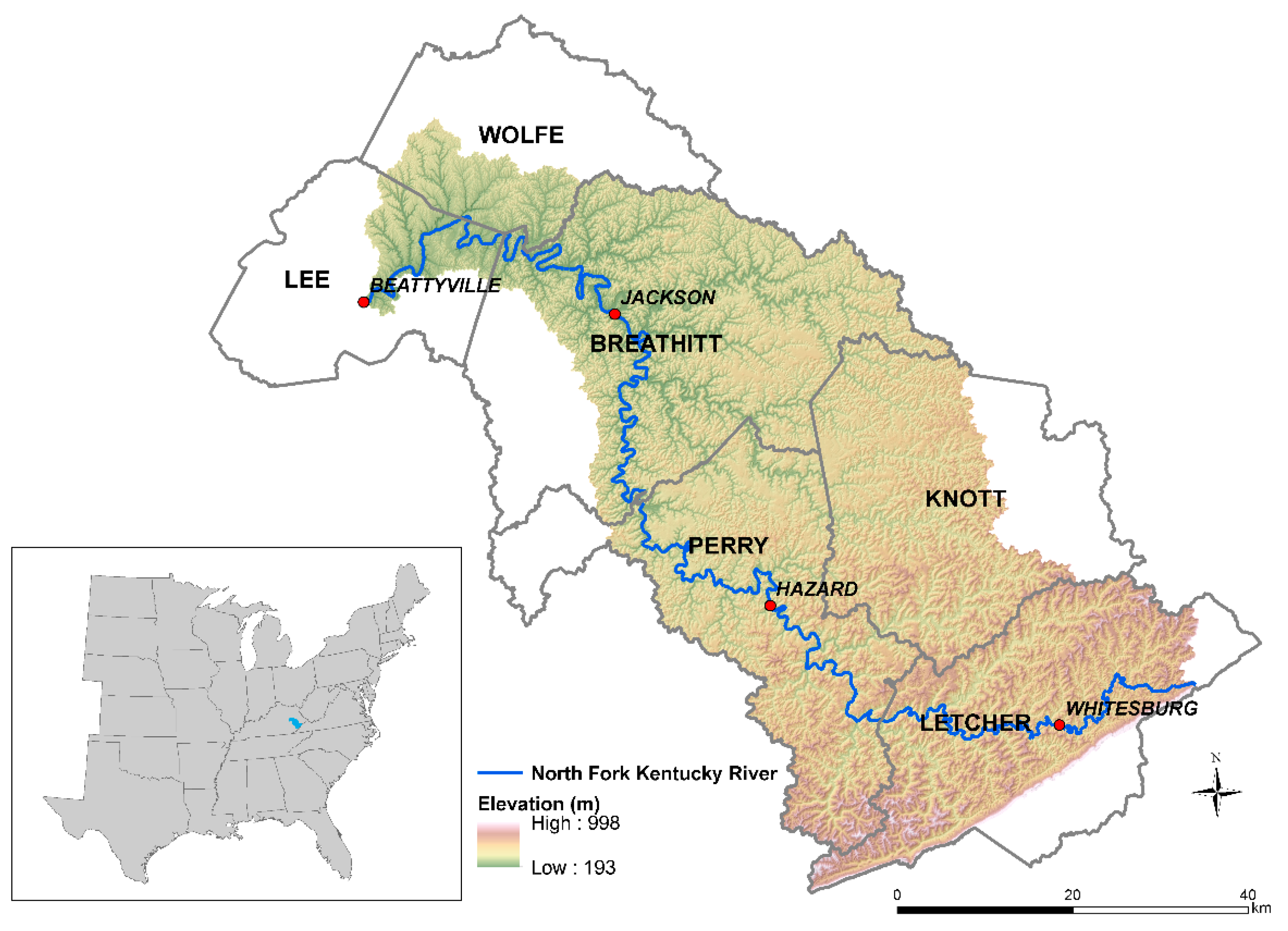
The North Fork Kentucky River (NFKR) watershed is situated in the Eastern Kentucky Coal Field physiographic region, which is part of a larger physiographic region, the Cumberland Plateau [30]. The watershed occupies most of Letcher, Perry, Knott, and Breathitt counties and a small portion of Lee County (Figure 1). These counties are part of the 65 counties in Central Appalachia where surface mining has been concentrated [14]. The welfare of many residents in Central Appalachia have been affected by surface mining in the past [31]. The NFKR watershed ranks among the groups with highest need for protection and restoration [30].
The watershed’s geology is comprised of coals, sandstones, and shales [30]. Land form is characterized by mountainous terrain, rapid surface runoff, and moderate rates of groundwater discharge [30]. Elevation ranges from 193 m to 998 m. The NFKR headwaters are allocated in Letcher County. The main stem of the river is 270 km long and flows northwest through the communities of Whitesburg, Hazard, and Jackson to reach Beattyville where it joins with the South Fork to form the Kentucky River (Figure 1).
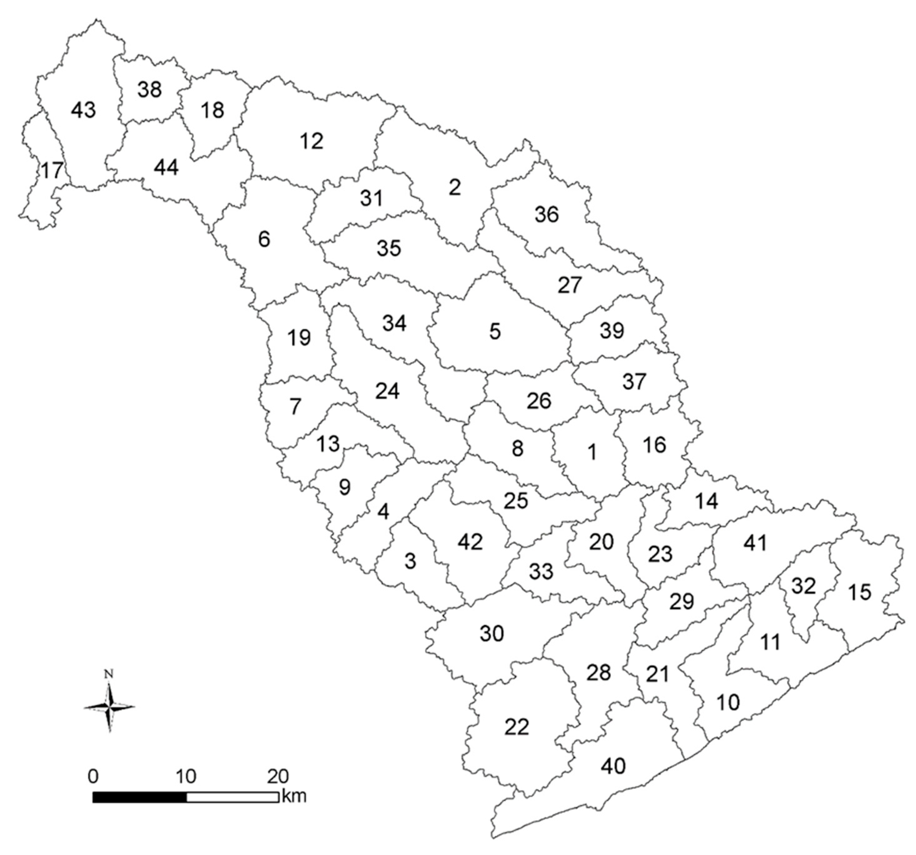
The NFKR watershed occupies a total area of approximately 3430 sq.km. There are 44 HUC-12 subwatersheds (Figure A1). HUC (Hydrologic Unit Code) is a scheme to describe hierarchy of watershed in the US, with HUC-2 representing the broadest region level and higher number of HUC digits representing spatially smaller levels. The size of the HUC-12 subwatersheds ranges from 38 sq. km to nearly 143 sq. km and the mean area is 76 sq. km (Table A1).
2.2. Land Cover Change Analysis
The Kentucky portion of the NLCD for 2001 and 2011 were obtained from the Kentucky Geography Network. The NLCD is a comprehensive Landsat-based, 30-m resolution land cover product. The NLCD has 16 land cover classifications applied across the continental United States. The first NLCD dataset was published for 1992, but its classification scheme does not match with that for the subsequent years of 2001 and forward, so the land covers of 2001 and 2011 (the latest available with the 2016 data are scheduled for release on 28 December 2018) have been chosen to study the land cover change over a decade.
The NLCD classification system is based on the Anderson Land Cover Classification System Level II [32]. There are generally a few Level-II LULC classes for each Level-I LULC type. For instance, LULC type Forest has three sub categories: Deciduous, Mixed, and Evergreen forest. Developed Land as a broad land cover has four sub categories with varying intensities (i.e., percentage) of impervious surfaces. These sub classes were aggregated into a single land cover type for simplicity in this research. In addition, the wetlands were aggregated with water class, and the cultivated crops were reclassified into pasture because there were negligible cultivated areas and visual comparison to the crop landscape dataset of CropScape [33] showed that most crops classified in the NLCD were pastures in this watershed.
The GIS data of watershed boundary was obtained from the National Hydrography Dataset (NHD). This watershed boundary data was used in the GIS operation Clip to extract NLCD data only for the NFKR watershed (Figure 1). The Not Equal operation in ArcGIS-Spatial Analyst toolbox was used to determine where in the watershed land cover has changed from 2001 to 2011. The output from this operation was a new raster layer in which cells/pixels valued 1 indicated land cover change and 0 indicated no change. To identify the magnitude of LULC changes among the 44 HUC-12 subwatersheds, a Zonal Statistics operation was performed on the output of Not Equal tool to compute the total number of cells/pixels that changed land cover within each subwatershed. Then the Join Field tool was used to join the contents of the zonal statistics table to the watershed shapefile for mapping the amount of area with LULC changes at the subwatershed level. The Tabulate Area operation was applied to calculate the LULC transiting matrix tabulating amount of area changing from one land cover type in 2001 to another in 2011. The transition matrix was then used to assess overall LULC changes in the entire watershed. To quantify the contribution of mining/reclamation to overall LULCC in this watershed, a separate LULC transition matrix was computed for only the areas where active mining was identified to have occurred at least one year from 2001 to 2011. This cumulatively mined area mask was derived from the annual mining extent dataset of Pericak et al. (2018) [34]. The contribution of mining and reclamation to the overall LULC change was based on the percentage of transitions from vegetated land covers to barren land and the transition from barren land to vegetated land cover types occurring within the cumulative mining area mask.
2.3. Ecosystem Services Assessment
The InVEST (Integrated Valuation of Ecosystem Services and Tradeoffs) software (InVEST 3.3.3, Natural Capital Project) was used to quantify the provision of four critical ecosystem services provided by the NFKR watershed under the most recently available LULC data (2011). InVEST software was developed by the Natural Capital Project, Stanford University [35]. It uses ecological production functions to generate spatially explicit predictions of ecosystem service supply with inputs of LULC maps, corresponding biophysical attributes, and additional GIS data representing environmental conditions such as climate, soil, and topography. For this study, InVEST’s Carbon Storage and Sequestration, Water Yield: Reservoir Hydropower Production, Sediment Delivery Ratio, and Nutrient Delivery Ratio (nitrogen and phosphorus) modules were used to estimate and map the annual delivery of the corresponding regulating services: carbon storage, flood control, soil retention, and surface water quality (Table 1). We chose to assess these four ecosystem services because they are characteristic regulating ecosystem services provided by the forests in Appalachian region that are important to human wellbeing but the degradation of these services due to deforestation are less obvious without a quantitative assessment.
- Carbon Storage and Sequestration
The InVEST carbon model aggregates the amount of carbon stored in four carbon pools: aboveground biomass, belowground biomass, soil, and dead organic matter to produce total amount of carbon storage. The input includes a user-defined biophysical attribute table (Table A2) that quantitatively describes each of these four biomass pools for each land use land cover type, and a LULC map. The model generates a map of total carbon storage by summing these four carbon pools for each grid cell based on its corresponding LULC type in million grams per hectare (mg per ha). In this study, the reclassified LULC map of NFKR watershed derived from NLCD 2011 was used as the input. The coefficient values used for the four carbon pools were from published data [36] and the InVEST manual (Table A2).
- Water Yield and Reservoir Hydropower Production
The InVEST water yield and reservoir hydropower production model estimates the total annual water yield (Y) for each pixel of the watershed as total annual precipitation minus total annual actual evapotranspiration [37]. The input of the water yield model includes five biophysical parameters as georeferenced raster inputs (Table A3). These inputs are precipitation (mm), average annual potential evapotranspiration (mm), depth to root restricting layer (mm), plant available water content (AWC, as a proportion), and LULC [38]. The precipitation data were obtained from the PRISM climate group of Oregon State University [39]. The precipitation data are 30-year Normal (1981–2010) dataset with a resolution of 800 m. The precipitation layer was resampled to a spatial resolution of 30 m by an interpolation method in ArcGIS. The PET was obtained from CGIAR-CSI website [40] (http://www.cgiar-csi.org). The depth to root restricting layer and the AWC were extracted from the SSURGO (Soil Survey Geographic database) [41] in the Soil Map viewer of the Web Soil Survey (USDA Natural Resources Conservation Service (NRCS). The LULC 2011 was obtained from the Kentucky Geoportal Network and its coordinate system was projected to meters.
The InVEST Water Yield model also requires several tabular values for each LULC class (Table A2). These values include an attribute indicating whether the land cover class is vegetated or not (1 being vegetated and 0 being not vegetated), maximum rooting depth for vegetated LULC and plant evapotranspiration coefficient (Kc). Kc is used to modify the reference evapotranspiration to obtain potential evapotranspiration. The reference ET is based on a 15 cm tall surface of actively growing, well-watered alfalfa. The plant ET coefficient (Kc) is a decimal number between 0 and 1.5 based on plant physiological characteristics. These tabular values (Table A2) were obtained from the biophysical attribute table compiled by Sharp et al. (2015) [37].
- Sediment Delivery Ratio (SDR)
The InVEST Sediment Delivery Ratio model quantifies average annual sediment delivery per subwatershed and produces a map representing per-pixel contribution to yield. For each pixel, the model first computes the amount of eroded sediment or soil loss based on precipitation pattern, soil properties, and topographic conditions. The model then estimates the sediment delivery ratio (proportion of soil loss reaching the subwatershed outlet) based on the pixel’s hydrologic connectivity [42] and further estimates sediment export based on the product of soil loss and sediment delivery ratio. The raster inputs required for the InVEST SDR model are a Digital Elevation Model (DEM), Rainfall Erosivity Index, Soil Erodibility, and LULC (Table A3). The DEM and LULC were derived from Kentucky Geoportal Network. The Rainfall Erosivity Index was obtained from European Soil Data Centre. The soil erodibility raster layer was acquired from the Soil Map Viewer program in GIS using SSURGO database. The tabular data needed for the SDR model includes biophysical parameters of cover management factor and support practice factor for the Universal Soil Loss Equation (USLE) (Table A2) [42]. These factors are floating-point values between 0 and 1 for each land cover. These biophysical parameters are from Sharp et al. (2015) [37].
- Nutrient Delivery Ratio (NDR)
The InVEST Nutrient Delivery Ratio (NDR) model aims to quantify nutrient export (nitrogen and phosphorus) and maps the transport of nutrients from watershed sources to the stream network. The model uses a mass balance approach, describing the long-term, steady flow of nutrients based on nutrient sources (nitrogen and phosphorus) associated with different LULC and the retention properties of pixels belonging to the same path [37]. The input raster layers required for the InVEST NDR model are DEM, LULC, and precipitation (Table A3). The DEM and LULC used are same as the SDR model inputs, obtained from the Kentucky Geoportal Network. The precipitation raster is from the PRISM Climatic Group of Oregon State University [39]. The tabular coefficient values for nitrogen and phosphorus loading for each land use category required (Table A2) are from Sharp et al. (2015) [37] and Line et al. (2002) [43], respectively.
2.4. FRA Scenario
To assess the ecological benefits brought by the FRA reclamation scenario, a new LULC map was created and used in InVEST models, while all other GIS input data and biophysical parameters were kept the same as the ecosystem service assessment of the contemporary LULC conditions. This scenario reflects a best-case scenario to provides a bench mark for us to assess the potential benefits gained by the FRA at watershed scales. The new LULC map was derived from NLCD 2011 map using the reclassification tool in ArcGIS in which all the barren, grassland, and shrubland were reclassified into forests. The ecosystem services indicators assessed in this scenario were carbon storage, water yield, sediment export, and nutrient export. The output of the various InVEST models were then analyzed in ArcGIS to examine differences in the biophysical indicators between this FRA scenario and the business as usual (BAE) scenario at the watershed level.
2.5. Statistical Analysis
To quantify the spatial heterogeneity of ecosystem services provision at the HUC-12 subwatershed level, a GIS zonal statistics operation was performed to compute mean value of the biophysical indicators within each subwatershed under both the contemporary and FRA scenarios. Zonal statistics was also applied with the 2011 land cover map to compute mean ecosystem services production of different land cover types. In addition, mean and standard deviation of elevation, slope steepness, precipitation, and percentage of forest land cover were computed at the subwatershed level, and were used as the explanatory variables in the subsequent driving factor analysis. Multiple linear regression (MLR) model was applied to evaluate the effect size and relative importance of LULC composition, topography, and climate in determining the spatial variability of the five biophysical indicators of ecosystem services under the FRA scenario. Since explanatory variables represent different biophysical properties, a scaling approach was used to standardize all variables into z-scores, which represents the distance between the raw value and the mean value in units of the standard deviation. After standardization, the effect size of each explanatory variable was quantified as the estimated slope from the MLR model. A model averaging method was used to estimate the slope of each explanatory variables to account for model selection uncertainty [44]. We used the “MuMIn” package in R 3.4.1 [45] to identify a set of alternative models whose delta Akaike Information Criterion (AIC) is less than 3. The relative importance of a given explanatory variable was quantified as the sum of Akaike weights over all of the selected models in which the term appeared [44,46].
3. Results
3.1. Land Cover Change
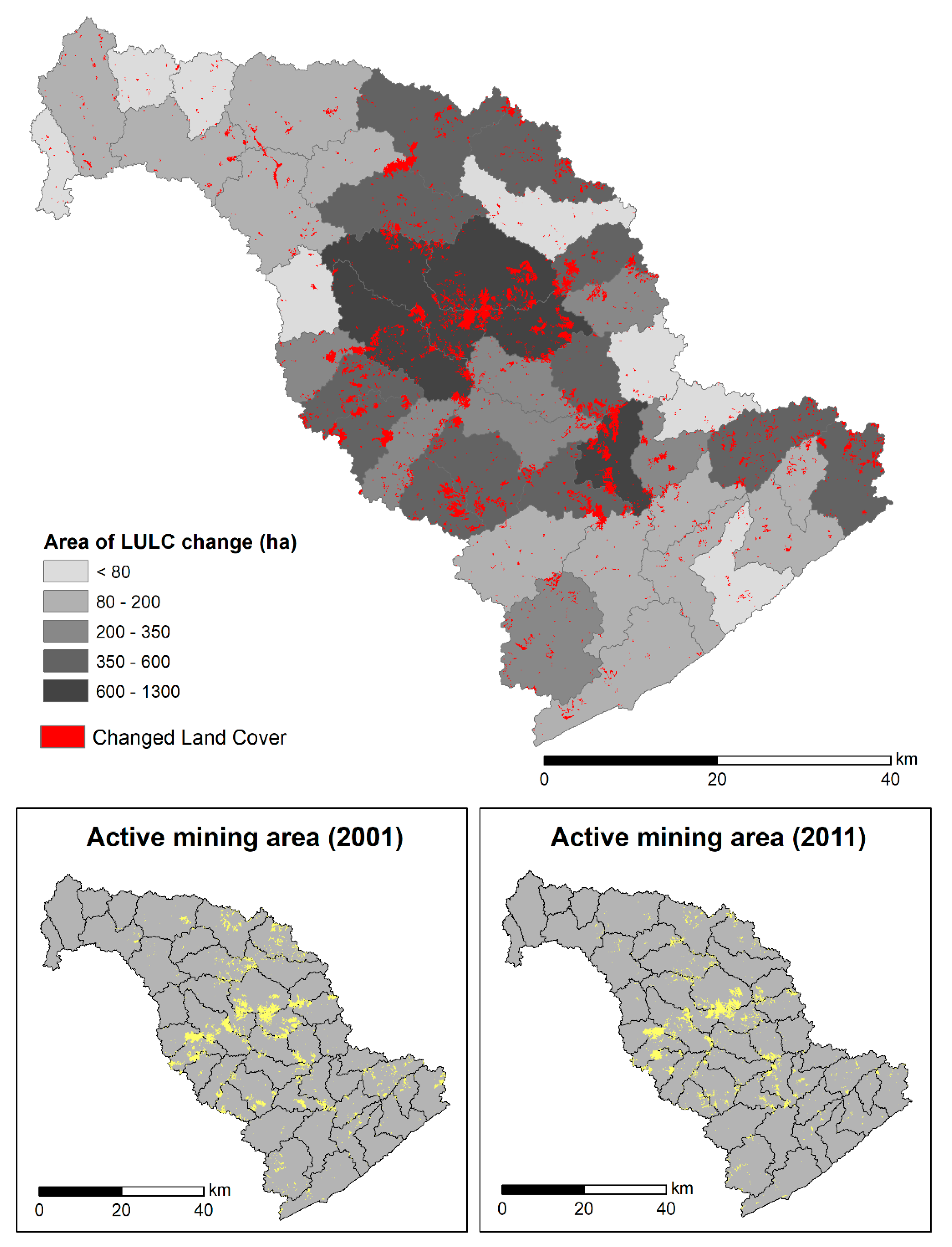
Six of the seven land use land cover categories increased their areal coverage between 2001 and 2011, only forest was reduced in its area (Table 2). The forest area reduction is notable, with a decline of 7751 hectares from 2001 (266,256 ha) to 2011 (258,505 ha). The loss in forests is accompanied with an increase in barren lands: 3844 hectare gain in 2011. Similarly, 3522 hectares of grasslands have been created. The area occupied by shrub land covers increased slightly by 53 hectares.
In terms of spatial distribution of land cover change, a distinct variability can be observed in the landscape. The subwatersheds at the central locations of the NFKR watershed generally experienced the greatest magnitude (>600 ha) of LULC changes (Figure 2). In addition, the size of these land cover change patches is quite large. The rest of the NFKR watershed is not free of land cover changes, with the subwatersheds located at the upper portions of the watershed (i.e., downstream of the North Fork Kentucky River) having the lowest magnitude of LULC changes. In addition, the land cover change patches are smaller in size and they are more spread out throughout the landscape (Figure 2).
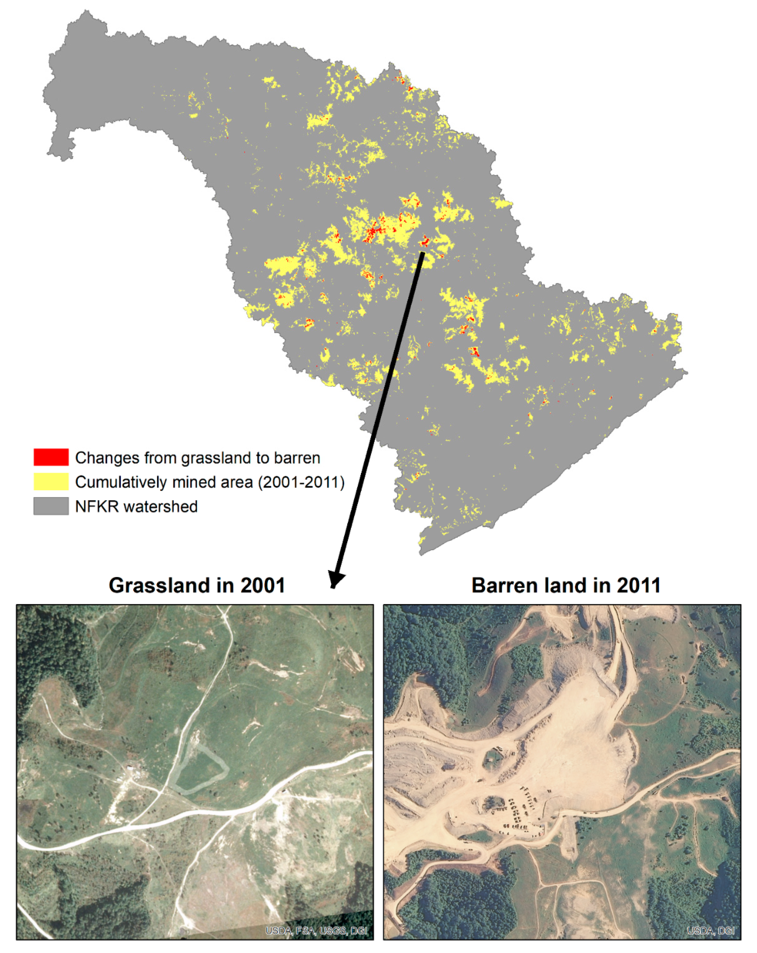
Of the total area of 342,895 hectares, 15,414 hectares of land covers were converted to other land cover categories between 2001 and 2011, which accounts for 4.5% of the watershed. The greatest transition is observed from forest in 2001 to barren land covers in 2011 (4840 hectares). This is followed by conversion of forest to grassland, where 4594 hectares of forest in 2001 are changed to grassland in 2011. The change of barren land covers to grassland cover is 2189 hectares in size (Table 3).
It is assumed that the transformation of forest to barren lands and grasslands, and barren to grasslands occurring in the cumulatively mined areas is due to mining and reclamation activities. The area of such LULC changes are 4125 ha, 2521 ha, and 2059 ha respectively (Table A4). The other noteworthy transition within the cumulatively mined areas is the conversion of grasslands to barren (1298 ha). This might be due to the fact that previously reclaimed mined areas are re-mined (Figure A2). These four types of land cover transitions within the mined areas make up a total of 9994 ha, which contribute approximately 65% of total land use land cover transitions that have occurred in the entire watershed. The results thus show mining and reclamation as a major driver of overall land use land cover change in the watershed.
3.2. Ecosystem Service Assessment under Contemporary LULC Conditions
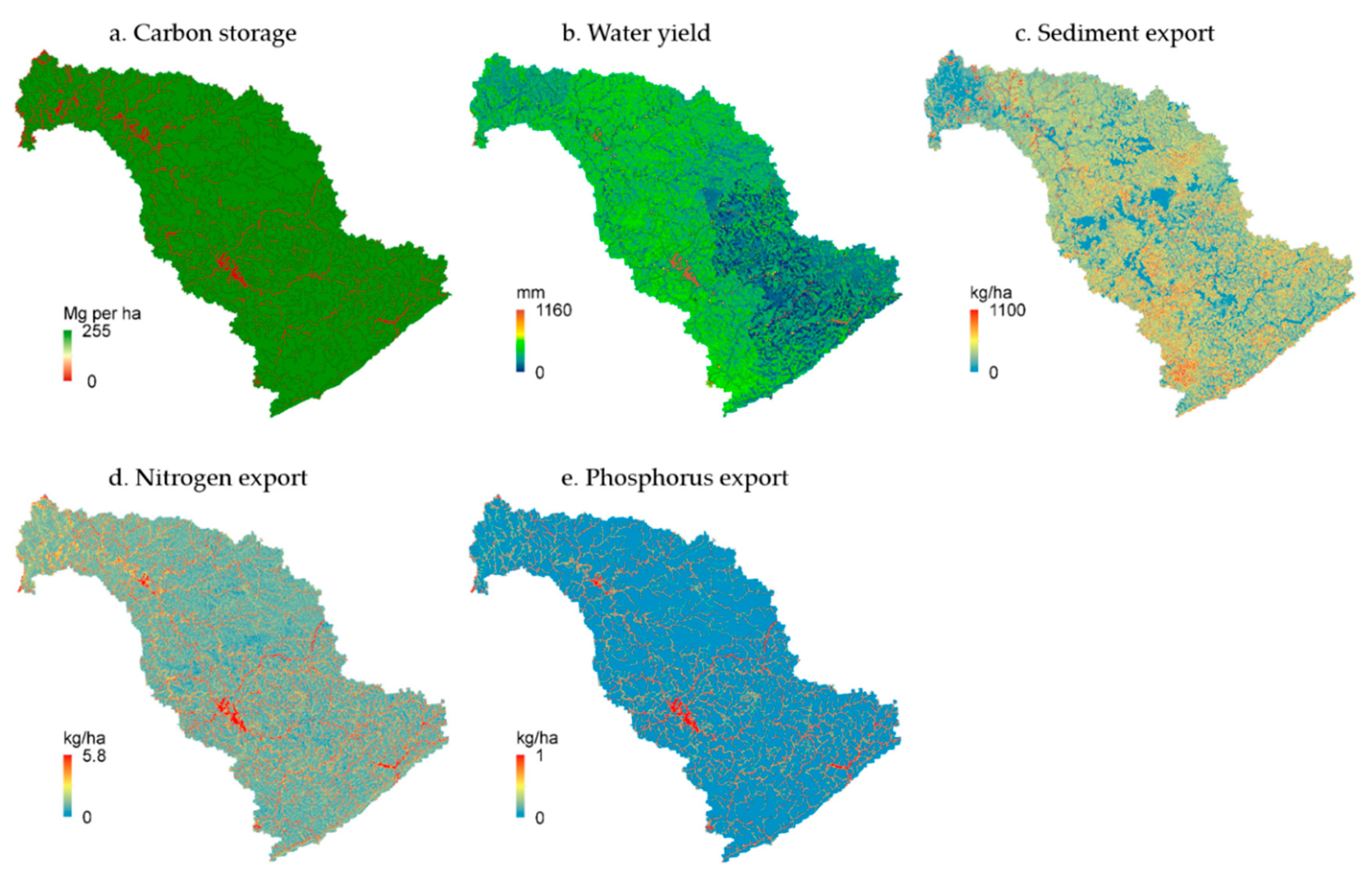
Ecosystem services production varied across the watershed, with the central locations of the watershed having lower ecosystem services production than other areas (Figure 3). Different land cover types produce different amount of ecosystem services. Forests generally produce greater ecosystem services than any other land cover types; they are associated with highest carbon storage and lowest water yield, sediment export, and nutrient export. In contrast, barren lands provide the lowest amount of ecosystem services among all non-urban land cover types; they produce lowest carbon storage and highest water yield, sediment export, and nutrient export (Table 4).
The total modeled carbon storage for the entire watershed is 71,343,168 mg. Mean carbon storage at the subwatershed level ranges from 138 mg per ha to 231 mg per ha (Table A5), with the lowest ranking subwatersheds occupying central locations of the watershed where surface mining is the most (Figure 3a). Carbon storage is highest in the forested lands with a mean of 250 mg per ha. The shrub land cover ranks second in storing carbon (100 mg per ha). Pasture ranks third with a carbon storage of 51 mg per ha. Grassland ranks fourth with a mean carbon storage of 45 mg per ha. Barren lands produce zero carbon storage (Table 4).
The total estimated water yield for the watershed is 2,219,528,435 mm. Mean water yield at the subwatershed level ranges 522 mm to 702 mm (Table A5), with the subwatersheds of highest mean water yield (hence lowest flood control capacity) occupying the central location in the watershed where the barren lands are concentrated (Figure 3b). Forested areas produce the least water yield (hence the greatest flood control capacity), with an average of 534 mm and grasslands have higher average water yield (665 mm) than the forests (Table 4).
Sediment export for the entire watershed is 52,848,288 kg. Mean sediment export ranges at the subwatershed level ranges from 101 kg per ha to 313 kg per ha (Table A5). The spatial distribution shows hotspots of sediment exports at the central locations of the watershed (Figure 3c). Among the land cover types, the barren areas have the highest mean sediment export (971 kg per ha). Pasture lands rank second with a mean sediment export of 628 kg per ha. The grasslands have a mean sediment export of 404 kg per ha. Forest land covers have the least mean sediment export (110 kg per ha) (Table 4).
The total nitrogen export of the entire watershed is 320,525 kg. Mean nitrogen export at the subwatershed level ranges from 0.67 kg per ha to 1.40 kg per ha (Table A5). The hotspots of nitrogen export are located around urban land covers (Figure 3d). Among all the five non-urban terrestrial land covers, nitrogen export is highest in barren areas (2 kg per ha), followed by pasture (1.6 kg per ha) and grassland (1.6 kg per ha) (Table 4). The forest and shrub lands both have least nitrogen export with a mean value of 0.5 kg per ha (Table 4).
The total phosphorus export for the watershed is 18,384 kg. Mean phosphorous export at the subwatershed ranges 0.027 kg per ha to 0.14 kg per ha (Table A5). Phosphorus export is highest in pasture (0.051 kg per ha) and then in grassland (0.02 kg per ha) (Table 4). Forest and shrub lands show a similar pattern, with a mean phosphorus export of 0.003 kg per ha. The barren lands have the least phosphorus export (0.001 kg per ha) (Table 4).
3.3. Ecosystem Service Assessment under FRA Scenario
Although more than 91% of the watershed was covered by forest under the forestry reclamation approach scenario, there are still conspicuous spatial variability of ecosystem service production (Figure 4), and the spatial patterns of ecosystem services differ from those under the contemporary LULC condition (Figure 4 vs. Figure 3). The spatial patterns under the FRA scenario largely reflect spatial configuration of LULC, particularly the juxtaposition between forest and developed land (i.e., urban and road networks). However, other driving factors such as topography and climate were also important contributors. Influences of forest land cover proportion, slope steepness, elevation, and precipitation on five biophysical indicators of ecosystem services at subwatershed level differed substantially in terms of both effect size and relative importance (Table 5). Forest land cover proportion was the sole important variable in explaining the variability of mean carbon storage among the 44 subwatersheds. Mean precipitation and slope, and standard deviation of slope steepness were the top three important variables and they all exerted positive influences (i.e., with positive slope coefficients in the model) on water yield. Sediment export was mainly determined by slope steepness, with steeper topographic slopes associated with higher amount of soil sediment. Forest land cover proportion was found to be the most important variable in explaining subwatershed level variations of nutrient export. The subwatersheds with higher forest land cover proportion were associated with lower export of nitrogen and phosphorous as the corresponding slope coefficients were negative values. Slope steepness and elevation had positive effects on the export of these two nutrients, but stronger effects were found on phosphorus than nitrogen (Table 5).
The benefits of forest reclamation approach, in comparison to the contemporary 2011 LULC scenario, are evident in terms of the production of all the ecosystem services assessed in this study. The total carbon storage of the watershed was estimated to be 80,633,377 mg of carbon under the FRA scenario. The difference is 9,290,209 mg of carbon which makes up an increase of 13% (Table 6) compared to the 2011 LULC scenario. The result suggests the climate regulation ecosystem service would be improved under FRA scenario. In addition, total water yield decreased by 5.2%, sediment export decreased by 40.5%, nitrogen export decreased by 22.6%, and phosphorous export decreased by 7.1% (Table 6), suggesting the watershed’s capacity in regulating flood, retaining soil, and maintain surface water quality would also be enhanced under the FRA scenario.
4. Discussion
This study investigated how LULC has changed in the NFKR watershed and the contribution of mining and reclamation to the overall land cover land use change, followed by the valuation of major ecosystem services under contemporary LULC conditions and the assessment of the benefits of the Forestry Reclamation Approach (FRA). The results show that even during a coal industry decline period, mining and reclamation are still prominent drivers shaping the structure and functions of many landscapes in Central Appalachia. Forests provide greater regulating ecosystem services than other land cover types, but the enhancement of ecosystem service production induced by forestry-based reclamation would differ for different types of ecosystem services and at different subwatersheds.
4.1. Surface Mining as a Prominent Driver of LULC Change
Rapid economic and social development since the industrial revolution has greatly geared up human demand for mineral resources. However, mining for these resources can cause extensive changes in LULC at landscape scales [47,48]. Coal is a primary energy source, and the three states from Appalachian area (Pennsylvania, West Virginia, and Kentucky) account for over 50% of the total coal production in the US [12]. It is estimated that more than 500,000 hectares of land have been mined for coals in this region [21]. Although coal production from Appalachian surface mining has declined by nearly 50% since its peak in 2008 due to depletion of high-quality coal seams, strict environmental regulation policy during the Obama administration era, and the collapse of coal mining industry [12]. A recent study that reconstructed mining activities across 30 years shows that cumulative mining area is continuing to expand in Central Appalachia, albeit at a much lower expansion rate [16]. The continuing expansion of cumulative mining area suggests that mining may still be a major driving force of the LULC change in some of the Appalachian landscapes, and this study demonstrates it is the case in the NFKR watershed. Based on the GIS analysis of the NLCD, the forested area was reduced by 7751 hectares (2.3% of the watershed) from 2001 to 2011 and barren and grassland LULCs increased 3844 and 3522 hectares, respectively (Table 2). A total of 15,414 hectares of land covers were converted to other land cover categories between 2001 and 2011, which accounts for 4.5% of the watershed. In contrast, within the cumulatively mined area of 29,189 ha, a total of 10,785 hectares of land with changing LULC, which accounts for 37% of mined area (Table A4). The forest land cover within the mining area decreased from 9675 ha in 2001 to 3539 ha in 2011, with a total reduction of 6136 ha, which accounts for 79% of forested area reduction at the watershed scale. Overall LULC changes and forest clearing were far more extensive within the cumulatively mined area than the surrounding area, suggesting mining is a major driver of LULC change in the NFKR watershed.
Our LULC change analyses show that areas changed from barren lands to grassland is much greater than the conversion of barren to forest. Only 179 hectares of barren lands in 2001 have converted to forest by 2011, whereas the conversion of barren lands to grasslands is 2189 hectares (Table 3). Tree plantation was prevalent in the abandoned mining sites prior to the SMCRA implementation, but reclamation to grassland became the dominant approach post-SMCRA [49]. Grasslands provide less regulating ecosystem services (e.g., climate regulation, flood control, and sediment retention) in comparison to forests. The InVEST modeling showed that grasslands have a mean carbon storage of 45 mg per ha, which is much less than what forests can store (250 mg per ha). Comparing to grassland, forests have lower mean water yield (534 vs. 665 mm), sediment export (110 vs. 404 kg per ha), nitrogen (0.5 vs. 1.6 kg per ha), and phosphorus export (0.001 vs. 0.02 kg per ha) than grasslands (Table 4). Although SMCRA mandates restoring the post-mining land to a condition capable of supporting the uses to the level similar to or higher than that prior to any mining, the majority of reclamation has failed to meet such standards when ecosystem services are considered as the evaluation criteria.
4.2. Ecosystem Services Assessment
Although ecosystem services are considered important, there is a lack of studies in Appalachia to evaluate how different land use and land cover might affect the provision of various ecosystem services. However, there are studies that are consistent with our findings that LULC changes driven by mining can significantly reduce the potential of a watershed to provide ecosystem services. According to Burkhard et al. (2009) [35], highly modified land cover types, such as mine sites, have very low or no relevant capacities to provide ecosystem services. Some studies have also stressed that unique impacts are brought about by mining, particularly by mountain top mining such as altering landform shape and structure and burying headwater streams [50]. All these changes adversely affect the functioning of ecosystems and results in reduced capacity of the landscape to regulate climate and flood, to retain sediments and nutrients, and to conserve and purify water.
The Millennium Ecosystem Assessment classifies ecosystem services into four categories, namely supporting, regulating, provisioning, and cultural ecosystem services. Our study only assessed the regulating ecosystem services because, unlike provisioning services such as food and timber production that are readily appreciated by the public, regulating ecosystem services are often overlooked in the decision-making as they do not have a market value. These regulating ecosystem services are critical in determining the production of many other ecosystem services and decline of these services foreshadows the decline of other ecosystem services [51]. Understanding the impacts of mining on the provision of critical regulating ecosystem services at landscape scales provide a better or understandable language to contribute positively to the formulation and evaluation of the relevant environmental policies [52,53].
The ecosystem assessment conducted with the InVEST modeling showed that even under a best-case reclamation scenario in which all the barren and grasslands were to be restored to forests, the enhancement of the regulating ecosystem services would still vary by ecosystem service type and subwatershed. This suggests that environmental benefits of forestry-based reclamation are landscape-specific and a thorough analysis regarding which ecosystem services need to be enhanced in which locations is warranted. In addition, forest based reclamation is not the only alternative or the best reclamation option in every mining site. An abandoned mining site can be reclaimed to grassland, pasture, agricultural land, etc. So trade-offs are bound to occur when the mining sites are reclaimed to various land uses. These trade-offs which arise from management choices can change the type, magnitude, and relative mix of ecosystem services provided by different ecosystems [54]. Reclamation would also require to consider land suitability. For example, mining sites that are close to developed areas may be more suitable to be developed to residential, commercial or industrial area and mining sites away from human settlement can be restored to forest [55]. The proper reclamation planning should consider both land suitability and ecosystem services that are needed to restore for the people living in the surrounding communities.
4.3. Limitations and Uncertainty
An important limitation of this study is the land cover dataset. The NLCD is a broad dataset and analysis for this study is for a relatively small spatial area of the continental scale dataset, so compromises are inherent in the classification of land use land covers. The NLCD classifications were based on the information from multiple years prior to 2001 and 2011, meaning classification used in the NLCD may not truly represent ground truth in all pixels for a given year. There are also known inaccuracies because of the techniques used to collect and classify the remotely sensed data. Some pixels identified as LULC change may be artifacts due to classification inaccuracies, not real changes. This is proven a major issue when conducting LULC change analysis with 1991 NLCD data, but a less serious issue with 2001 and 2011 NLCD data [56]. Generally, the patches misclassified as LULC changes are small in size, and should have negligible impacts when assessing major LULC transitions at landscape scales.
The InVEST software has its own modeling limitations. For the InVEST Carbon Storage and Sequestration Model, the model only estimates the temporally average carbon storage for each LULC hence assumes that none of the LULC types in the landscape are gaining or losing carbon over time. Changes in carbon storage simulated in this model can only be induced by the changes from one land cover type to another. The InVEST Water Yield and Reservoir Hydropower Production Model is based on annual averages, which neglects extremes and does not consider the temporal dimensions of water supply. It does not consider complex land use patterns or underlying geology, which may induce complex water balances. The main limitation of the InVEST Sediment Delivery Ration Model is its reliance on the Universal Soil Loss Equation. Even though this equation is widely used, it only represents rill erosion process, which is the removal of soil by concentrated water running through little streamlets. The InVEST Nutrient Delivery Ration Model is highly sensitive to inputs, so small errors in the empirical load parameter, will have a large effect on predictions of nutrient delivery. The tabular values used are not entirely from the study area because of data limitation in the study area; they have been acquired from published sources and the master table of the InVEST manual.
This study assumed that the FRA forests on the abandoned mining sites can provide regulating ecosystem services at a similar level to the natural forests on the unmined sites. This assumption was made to assess the ecological benefits at a best-case scenario. Although site conditions on those FRA forests are altered via mining, field studies of FRA effects show that forests reclaimed on the mining sites can quickly recover many important ecological processes characteristic of the native forest ecosystems [20]. This is particularly the case for the processes related to regulating ecosystem services. For example, because the FRA emphasizes replacement of loose soil materials, FRA reclamation practices can help the mine site “evolve” hydrologically, developing infiltration/runoff patterns more like unmined landscapes with time [24,57].
For the ecosystem service assessment conducted in this study, a major implication is for the authorities and the general public to appreciate the value of ecosystem services; to gain knowledge about the loss of ecosystem services due to land conversions like mining, and the potential improvement in the delivery of ecosystem services when forest-oriented reclamation practices are applied. This study adds a block to the ecosystem services’ study of Appalachia as such studies are scarce in this region. The outcomes presented in tables and maps illustrate different land cover types have different capacity in providing ecosystem services, and the spatial characteristics of LULC, topography, and climate are important drivers of the provision of ecosystem services at watershed and subwatershed levels. The maps produced in this study provide important spatially explicit information to support managers to identify areas where the ecosystems are produced in larger quantities and where they are not. Despite model and data limitations, this study can be helpful in enforcing and popularizing reclamation strategies like the forestry reclamation approach and prioritizing locations for restoration at landscape scales.
5. Conclusions
Assessing ecosystem services under different land use land cover conditions can provide critical information regarding the benefits of the ecological restoration. Such information is helpful in the decision-making process for achieving landscape sustainability. In mountainous areas such as the Appalachian region, the change of LULC is often extensive and intensive due to the large-scale extraction of natural resources, and this study demonstrated the extent of this land degradation problem and its cascading effects on ecosystem services provision in an Appalachian watershed. Comparing to current reclamation strategies in which most abandoned mined sites are reclaimed to grassland, forestry-based reclamation can greatly enhance the provision of many regulating ecosystem services, particularly sediment retention and water purification. It further showed that the different types of ecosystem services can have different response to the forestry-based reclamation strategy, and the spatial heterogeneity of ecosystem services provision is largely driven by LULC composition, topographic variability and climate. The results showcase the importance of considering landscape ecology and land change science in ecosystem service assessment and policy-making of mined land restoration.
Author Contributions
J.Y. conceived and designed the study. K.G. and L.F. analyzed data. K.G., J.Y., and L.F. wrote the manuscript.
Funding
This work was funded by the University of Kentucky and the USDA National Institute of Food and Agriculture, McIntire Stennis project 1014537.
Acknowledgments
The authors would like to thank Bai Yang for his expert help in this research. We are grateful to Chase Clark, senior GIS analyst for helping K.G. with GIS mappings and processing. We also would like to thank Brian Lee, Mary Arthur, and Marco Contreras for their valuable inputs in K.G.’s Master’s thesis that helped improve this manuscript. This is publication No. 18-09-091 of the Kentucky Agricultural Experiment Station and is published with the approval of the Director.
Conflicts of Interest
The authors declare no conflicts of interest.
Appendix A
Figure A1.
Subwatersheds of the NFKR watershed.


Table A1.
The ID, name, area, and HUC of the 44 Subwatersheds in the NFKR watershed.
| ID | Name | Area Sq. km | HUC Code |
|---|---|---|---|
| 1 | Big Branch-Troublesome Creek | 60 | 51002010502 |
| 2 | Big Caney Creek-Quicksand Creek | 122 | 51002010604 |
| 3 | Big Creek | 51 | 51002010306 |
| 4 | Big Willard Creek-North Fork Kentucky River | 61 | 51002010401 |
| 5 | Buckhorn Creek | 118 | 51002010506 |
| 6 | Cane Creek-North Fork Kentucky River | 119 | 51002010701 |
| 7 | Caney Creek-North Fork Kentucky River | 50 | 51002010404 |
| 8 | Clear Creek-Troublesome Creek | 63 | 51002010503 |
| 9 | Colwell Fork-North Fork Kentucky River | 48 | 51002010402 |
| 10 | Cowan Creek-North Fork Kentucky River | 73 | 51002010104 |
| 11 | Crafts Colly Creek-North Fork Kentucky River | 75 | 51002010103 |
| 12 | Frozen Creek | 142 | 51002010702 |
| 13 | Grapevine Creek-North Fork Kentucky River | 60 | 51002010403 |
| 14 | Headwaters Carr Fork | 48 | 51002010201 |
| 15 | Headwaters North Fork Kentucky River | 79 | 51002010101 |
| 16 | Headwaters Troublesome Creek | 61 | 51002010501 |
| 17 | Hell Creek-North Fork Kentucky River | 38 | 51002010707 |
| 18 | Holly Creek | 50 | 51002010703 |
| 19 | Howards Creek-North Fork Kentucky River | 61 | 51002010405 |
| 20 | Irishman Creek-Carr Fork | 64 | 51002010203 |
| 21 | Kings Creek-North Fork Kentucky River | 75 | 51002010105 |
| 22 | Leatherwood Creek | 129 | 51002010303 |
| 23 | Little Carr Fork-Carr Fork | 53 | 51002010202 |
| 24 | Lost Creek | 110 | 51002010507 |
| 25 | Lotts Creek | 73 | 51002010305 |
| 26 | Lower Balls Fork | 58 | 51002010505 |
| 27 | Lower Laurel Fork Quicksand Creek-Quicksand Creek | 95 | 51002010602 |
| 28 | Lower Line Fork-North Fork Kentucky River | 99 | 51002010302 |
| 29 | Lower Rockhouse Creek | 57 | 51002010107 |
| 30 | Maces Creek-North Fork Kentucky River | 111 | 51002010304 |
| 31 | Meatscaffold Branch-Quicksand Creek | 60 | 51002010606 |
| 32 | Millstone Creek-North Fork Kentucky River | 38 | 51002010102 |
| 33 | Montgomery Creek-Carr Fork | 56 | 51002010204 |
| 34 | Russell Branch-Troublesome Creek | 107 | 51002010508 |
| 35 | South Fork Quicksand Creek | 104 | 51002010605 |
| 36 | Spring Fork Quicksand Creek | 92 | 51002010603 |
| 37 | Upper Balls Fork | 59 | 51002010504 |
| 38 | Upper Devil Creek | 45 | 51002010705 |
| 39 | Upper Laurel Fork Quicksand Creek | 53 | 51002010601 |
| 40 | Upper Line Fork | 122 | 51002010301 |
| 41 | Upper Rockhouse Creek | 88 | 51002010106 |
| 42 | Upper Second Creek-North Fork Kentucky River | 86 | 51002010307 |
| 43 | Walker Creek-North Fork Kentucky River | 113 | 51002010706 |
| 44 | War Creek-North Fork Kentucky River | 104 | 51002010704 |
Table A2.
Carbon pool estimates and other biophysical attributes used for the InVEST models.
| LULC | ||||||||
|---|---|---|---|---|---|---|---|---|
| Biophysical Attributes | Developed | Barren | Forest | Shrubland | Grassland | Pasture | Source | Related Models |
| Aboveground biomass | 5 | 0 | 90 | 30 | 10 | 10 | Sharp et al. (2015), Qiu and Turner (2013) | Carbon Storage |
| Belowground biomass | 3 | 0 | 60 | 20 | 5 | 11 | ||
| Soil organic matter | 20 | 0 | 75 | 40 | 20 | 20 | ||
| Dead organic matter | 0 | 0 | 25 | 10 | 10 | 10 | ||
| Kc | 0.1 | 0.2 | 1 | 0.85 | 0.65 | 0.85 | Sharp et al. (2015) | Water Yield |
| Root_depth | 300 | 10 | 7000 | 4750 | 2000 | 1000 | ||
| usle_c | 0.001 | 0.25 | 0.003 | 0.003 | 0.01 | 0.02 | Sharp et al. (2015) | Sediment Delivery |
| usle_p | 0.001 | 0.01 | 0.2 | 0.2 | 0.2 | 0.25 | ||
| load_n | 7.75 | 4 | 1.8 | 1.8 | 4 | 3.1 | Line et al. (2002), Sharp et al. (2015) | Nutrient Delivery |
| load_p | 1.3 | 0.001 | 0.001 | 0.011 | 0.05 | 0.1 | ||
The carbon storage estimates for the four carbon pools is measured in mg per ha. Kc is the plant evapotranspiration coefficient. Root depth is the maximum root depth (mm) for vegetated land use land covers. usle_c and usle_p are the cover management factor and support practice factor for the USLE respectively. Load_n and load_p are the nutrient loading for each land use (kg per ha per year).
Table A3.
GIS data layers needed for the InVEST models.
| Required GIS Data | Description | Source | Related Models |
|---|---|---|---|
| Land Use Land Cover (LULC) | Land cover classification scheme at 30 m resolution. | National Land Cover Database, https://www.mrlc.gov | All |
| Digital Elevation Model (DEM) | A raster dataset with an elevation value for each cell. | Kentucky Geographic Network, kygisserver.ky.gov/geoportal | Sediment Delivery, Nutrient Delivery |
| Rainfall Erosivity Index | A raster with an erosivity value for each cell; depends on the intensity and duration of rainfall. | European Soil Data Centre, https://esdac.jrc.ec.europa.eu | Sediment Delivery |
| Soil Erodibility | A measure of susceptibility of soil particles to detachment and transport by rainfall and runoff. | Soil Map Viewer, NRCS, https://websoilsurvey.nrcs.usda.gov/ | Sediment Delivery |
| Depth to root restricting layer | A raster dataset with an average root restricting layer depth value (mm) for each cell. | Soil Map Viewer, NRCS, https://websoilsurvey.nrcs.usda.gov/ | Water Yield |
| Annual average precipitation | A raster with a non- zero value for average annual precipitation. (mm). | PRISM Climate Data-Oregon State University, prism.oregonstate.edu/ | Sediment Delivery, Nutrient Delivery, Water Yield |
| Reference evapotranspiration | The potential loss of water from the soil by both evapotranspiration from the soil and transpiration by healthy alfalfa (grass) if sufficient water is available (mm). | Consortium for Spatial Information (CGIAR CSI), http://www.cgiar-csi.org/data/global-aridity-and-pet-database | Water Yield |
| Plant available water content | The fraction of water that can be stored in the soil profile for plants’ use. | Soil Map Viewer, NRCS, https://websoilsurvey.nrcs.usda.gov/ | Water Yield |
| Watersheds and subwatersheds | A layer of watersheds such that each watershed contributes to a point of interest where water quality will be analyzed. | National Hydrography Dataset, https://nhd.usgs.gov | Sediment Delivery, Nutrient Delivery, Water Yield |
Table A4.
Size of area that has experienced transition from one land cover category to another between 2001 and 2011 (unit, hectares) within the mined sites in the NFKR watershed.
Table A4.
Size of area that has experienced transition from one land cover category to another between 2001 and 2011 (unit, hectares) within the mined sites in the NFKR watershed.
| 2011 | |||||||||
|---|---|---|---|---|---|---|---|---|---|
| 2001 | LULC | Water | Developed | Barren | Forest | Shrub | Grassland | Pasture | Total |
| Water | 147 | 0 | 11 | 2 | 0 | 8 | 0 | 168 | |
| Developed | 0 | 1314 | 0 | 0 | 0 | 0 | 0 | 1314 | |
| Barren | 25 | 9 | 4683 | 145 | 1 | 2059 | 3 | 6925 | |
| Forest | 13 | 41 | 4125 | 2968 | 1 | 2521 | 6 | 9675 | |
| Shrub | 0 | 1 | 8 | 1 | 16 | 2 | 1 | 29 | |
| Grassland | 15 | 53 | 1298 | 422 | 4 | 9132 | 1 | 10,925 | |
| Pasture | 0 | 1 | 1 | 1 | 0 | 6 | 144 | 53 | |
| Total | 200 | 1419 | 10,126 | 3539 | 22 | 13,728 | 155 | 29,189 | |
Figure A2.
An example of land conversion from grassland in 2001 to barren in 2011.

Table A5.
Mean ecosystem service production per subwatershed under 2011 LULC conditions.
| Biophysical Indicators of Ecosystem Services | ||||||
|---|---|---|---|---|---|---|
| ID | Subwatersheds | Carbon Storage (mg per ha) | Water Yield (mm) | Sediment Export (kg per ha) | Nitrogen Export (kg per ha) | Phosphorus Export (kg per ha) |
| 1 | Big Branch-Troublesome Creek | 182 | 582 | 221 | 1.06 | 0.065 |
| 2 | Big Caney Creek-Quicksand Creek | 210 | 617 | 129 | 0.79 | 0.038 |
| 3 | Big Creek | 180 | 680 | 313 | 1.08 | 0.058 |
| 4 | Big Willard Creek-North Fork Kentucky River | 186 | 672 | 204 | 1.14 | 0.091 |
| 5 | Buckhorn Creek | 191 | 611 | 235 | 0.88 | 0.027 |
| 6 | Cane Creek-North Fork Kentucky River | 210 | 620 | 127 | 0.92 | 0.065 |
| 7 | Caney Creek-North Fork Kentucky River | 198 | 636 | 176 | 0.88 | 0.036 |
| 8 | Clear Creek-Troublesome Creek | 181 | 601 | 202 | 1.07 | 0.069 |
| 9 | Colwell Fork-North Fork Kentucky River | 176 | 677 | 236 | 1.11 | 0.061 |
| 10 | Cowan Creek-North Fork Kentucky River | 218 | 536 | 126 | 0.82 | 0.052 |
| 11 | Crafts Colly Creek-North Fork Kentucky River | 206 | 560 | 132 | 1.04 | 0.087 |
| 12 | Frozen Creek | 228 | 608 | 115 | 0.75 | 0.036 |
| 13 | Grapevine Creek-North Fork Kentucky River | 138 | 702 | 263 | 1.32 | 0.066 |
| 14 | Headwaters Carr Fork | 217 | 522 | 150 | 0.82 | 0.049 |
| 15 | Headwaters North Fork Kentucky River | 198 | 564 | 201 | 1.02 | 0.072 |
| 16 | Headwaters Troublesome Creek | 216 | 554 | 140 | 0.86 | 0.056 |
| 17 | Hell Creek-North Fork Kentucky River | 187 | 622 | 117 | 1.01 | 0.069 |
| 18 | Holly Creek | 215 | 558 | 172 | 0.9 | 0.053 |
| 19 | Howards Creek-North Fork Kentucky River | 230 | 597 | 112 | 0.71 | 0.039 |
| 20 | Irishman Creek-Carr Fork | 169 | 548 | 291 | 1.02 | 0.047 |
| 21 | Kings Creek-North Fork Kentucky River | 212 | 532 | 163 | 0.85 | 0.05 |
| 22 | Leatherwood Creek | 209 | 653 | 214 | 0.86 | 0.047 |
| 23 | Little Carr Fork-Carr Fork | 208 | 525 | 151 | 0.85 | 0.055 |
| 24 | Lost Creek | 181 | 656 | 230 | 1.01 | 0.048 |
| 25 | Lotts Creek | 198 | 589 | 193 | 0.98 | 0.069 |
| 26 | Lower Balls Fork | 136 | 615 | 278 | 1.25 | 0.053 |
| 27 | Lower Laurel Fork Quicksand Creek-Quicksand Creek | 222 | 567 | 134 | 0.67 | 0.029 |
| 28 | Lower Line Fork-North Fork Kentucky River | 219 | 542 | 117 | 0.8 | 0.047 |
| 29 | Lower Rockhouse Creek | 192 | 529 | 173 | 1.02 | 0.076 |
| 30 | Maces Creek-North Fork Kentucky River | 218 | 621 | 176 | 0.83 | 0.051 |
| 31 | Meatscaffold Branch-Quicksand Creek | 220 | 621 | 134 | 0.81 | 0.048 |
| 32 | Millstone Creek-North Fork Kentucky River | 196 | 548 | 199 | 0.95 | 0.058 |
| 33 | Montgomery Creek-Carr Fork | 181 | 616 | 247 | 1.02 | 0.056 |
| 34 | Russell Branch-Troublesome Creek | 190 | 631 | 232 | 0.91 | 0.04 |
| 35 | South Fork Quicksand Creek | 201 | 623 | 128 | 0.8 | 0.031 |
| 36 | Spring Fork Quicksand Creek | 191 | 617 | 181 | 0.85 | 0.032 |
| 37 | Upper Balls Fork | 194 | 578 | 181 | 0.96 | 0.057 |
| 38 | Upper Devil Creek | 200 | 586 | 145 | 1 | 0.061 |
| 39 | Upper Laurel Fork Quicksand Creek | 196 | 582 | 179 | 0.86 | 0.026 |
| 40 | Upper Line Fork | 231 | 577 | 123 | 0.75 | 0.042 |
| 41 | Upper Rockhouse Creek | 190 | 558 | 246 | 0.97 | 0.053 |
| 42 | Upper Second Creek-North Fork Kentucky River | 172 | 698 | 196 | 1.4 | 0.146 |
| 43 | Walker Creek-North Fork Kentucky River | 199 | 588 | 101 | 0.94 | 0.052 |
| 44 | War Creek-North Fork Kentucky River | 210 | 591 | 124 | 0.89 | 0.049 |
References
- Turner, M.G.; Hargrove, W.W.; Gardner, R.H.; Romme, W.H. Effects of fire on landscape heterogeneity in Yellowstone national park, Wyoming. J. Veg. Sci. 1994, 5, 731–742. [Google Scholar] [CrossRef]
- Houghton, R.A. The worldwide extent of land-use change. BioScience 1994, 44, 305–313. [Google Scholar] [CrossRef]
- Turner, B.L.; Lambin, E.F.; Reenberg, A. The emergence of land change science for global environmental change and sustainability. Proc. Natl. Acad. Sci. USA 2007, 104, 20666–20671. [Google Scholar] [CrossRef] [PubMed] [Green Version]
- Foley, J.A.; DeFries, R.; Asner, G.P.; Barford, C.; Bonan, G.; Carpenter, S.R.; Chapin, F.S.; Coe, M.T.; Daily, G.C.; Gibbs, H.K.; et al. Global consequences of land use. Science 2005, 309, 570–574. [Google Scholar] [CrossRef] [PubMed]
- Lambin, E.F.; Turner, B.L.; Geist, H.J.; Agbola, S.B.; Angelsen, A.; Bruce, J.W.; Coomes, O.T.; Dirzo, R.; Fischer, G.; Folke, C.; et al. The causes of land-use and land-cover change: Moving beyond the myths. Glob. Environ. Change 2001, 11, 261–269. [Google Scholar] [CrossRef]
- Vitousek, P.M.; Mooney, H.A.; Lubchenco, J.; Melillo, J.M. Human domination of earth’s ecosystems. Science 1997, 277, 494–499. [Google Scholar] [CrossRef]
- Guo, L.B.; Gifford, R. Soil carbon stocks and land use change: A meta analysis. Glob. Change Biol. 2002, 8, 345–360. [Google Scholar] [CrossRef]
- Shrestha, R.K.; Lal, R. Changes in physical and chemical properties of soil after surface mining and reclamation. Geoderma 2011, 161, 168–176. [Google Scholar] [CrossRef]
- DeFries, R.; Eshleman, K.N. Land-use change and hydrologic processes: A major focus for the future. Hydrol. Process. 2004, 18, 2183–2186. [Google Scholar] [CrossRef]
- Wu, J. Landscape sustainability science: Ecosystem services and human well-being in changing landscapes. Landsc. Ecol. 2013, 28, 999–1023. [Google Scholar] [CrossRef]
- Encyclopaedia Britannica. Available online: https://www.britannica.com/technology/mining (accessed on 12 January 2018).
- Höök, M.; Aleklett, K. Historical trends in American coal production and a possible future outlook. Int. J. Coal Geol. 2009, 78, 201–216. [Google Scholar] [CrossRef]
- U.S. Environmental Protection Agency. The effects of mountaintop mines and valley fills on aquatic ecosystems of the central appalachian coalfields. In USEPA; Washington, DC, EPA/600/R-09/138F; 2011. Available online: https://cfpub.epa.gov/ncea/risk/recordisplay.cfm?deid=225743 (accessed on 17 March 2018).
- Wickham, J.; Wood, P.B.; Nicholson, M.C.; Jenkins, W.; Druckenbrod, D.; Suter, G.W.; Strager, M.P.; Mazzarella, C.; Galloway, W.; Amos, J. The overlooked terrestrial impacts of mountaintop mining. BioScience 2013, 63, 335–348. [Google Scholar] [CrossRef]
- Bernhardt, E.S.; Palmer, M.A. The environmental costs of mountaintop mining valley fill operations for aquatic ecosystems of the central Appalachians. Ann. N. Y. Acad. Sci. 2011, 1223, 39–57. [Google Scholar] [CrossRef] [PubMed]
- Lindberg, T.T.; Bernhardt, E.S.; Bier, R.; Helton, A.; Merola, R.B.; Vengosh, A.; Di Giulio, R.T. Cumulative impacts of mountaintop mining on an Appalachian watershed. Proc. Natl. Acad. Sci. USA 2011, 108, 20929–20934. [Google Scholar] [CrossRef] [PubMed] [Green Version]
- Dickens, P.S.; Tschantz, B.A.; Minear, R.A. Sediment yield and water quality from a steep-slope surface mine spoil. Trans. ASAE 1985, 28, 1838–1845. [Google Scholar] [CrossRef]
- Miller, J.; Barton, C.; Agouridis, C.; Fogel, A.; Dowdy, T.; Angel, P. Evaluating soil genesis and reforestation success on a surface coal mine in Appalachia. Soil Sci. Soc. Am. J. 2012, 76, 950–960. [Google Scholar] [CrossRef]
- Fox, J.F.; Campbell, J.E. Terrestrial carbon disturbance from mountaintop mining increases lifecycle emissions for clean coal. Environ. Sci. Technol. 2010, 44, 2144–2149. [Google Scholar] [CrossRef] [PubMed]
- Zipper, C.E.; Burger, J.A.; Skousen, J.G.; Angel, P.N.; Barton, C.D.; Davis, V.; Franklin, J.A. Restoring forests and associated ecosystem services on Appalachian coal surface mines. Environ. Manag. 2011, 47, 751–765. [Google Scholar] [CrossRef] [PubMed]
- Perks, R. Appalachian Heartbreak: Time to End Mountaintop Removal Coal Mining. Natural Resources Defense Council, 26. 2013. Available online: http://www.nrdc.org/land/appalachian/files/appalachian.pdf (accessed on 26 June 2010).
- Burger, J.; Graves, D.; Angel, P.; Davis, V.; Zipper, C. Appalachian Regional Reforestation Initiative. Forestry Reclamation Advisory no. 2. The Forestry Reclamation Approach; 2005. Available online: https://www.epa.gov/cwa-404/appalachian-stream-mitigation-workshop (accessed on 10 July 2016).
- Angel, P.N.; Burger, J.A.; Davis, V.M.; Barton, C.D.; Bower, M.; Eggerud, S.D.; Rothman, P. The forestry reclamation approach and the measure of its success in Appalachia. Proc. Am. Soc. Min. Reclam. 2009, 20091, 18–36. [Google Scholar]
- Sena, K.; Barton, C.; Angel, P.; Agouridis, C.; Warner, R. Influence of spoil type on chemistry and hydrology of interflow on a surface coal mine in the eastern US coalfield. Water Air Soil Pollut. 2014, 225, 2171. [Google Scholar] [CrossRef]
- Wilson-Kokes, L.; Emerson, P.; DeLong, C.; Thomas, C.; Skousen, J. Hardwood tree growth after eight years on brown and gray mine soils in West Virginia. J. Environ. Qual. 2013, 42, 1353–1362. [Google Scholar] [CrossRef] [PubMed]
- Daily, G.C.; Söderqvist, T.; Aniyar, S.; Arrow, K.; Dasgupta, P.; Ehrlich, P.R.; Folke, C.; Jansson, A.; Jansson, B.-O.; Kautsky, N.; et al. The value of nature and the nature of value. Science 2000, 289, 395–396. [Google Scholar] [CrossRef] [PubMed]
- Berkes, F.; Folke, C. (Eds.) Linking Social and Ecological Systems: Management Practices and Social Mechanisms for Building Resilience; Cambridge University Press: Cambridge, UK, 1998; Volume 1, pp. 285–310. [Google Scholar]
- Benayas, J.M.R.; Newton, A.C.; Diaz, A.; Bullock, J.M. Enhancement of biodiversity and ecosystem services by ecological restoration: A meta-analysis. Science 2009, 325, 1121–1124. [Google Scholar] [CrossRef] [PubMed]
- Nelson, E.; Mendoza, G.; Regetz, J.; Polasky, S.; Tallis, H.; Cameron, D.; Chan, K.M.; Daily, G.C.; Goldstein, J.; Kareiva, P.M.; et al. Modeling multiple ecosystem services, biodiversity conservation, commodity production, and tradeoffs at landscape scales. Front. Ecol. Environ. 2009, 7, 4–11. [Google Scholar] [CrossRef] [Green Version]
- Haag, K.H.; Porter, S.D. Water-Quality Assessment of the Kentucky River Basin, Kentucky: Nutrients, Sediments, and Pesticides in Streams, 1987-90; US Department of the Interior, US Geological Survey: Louisville, KY, USA, 1995.
- Hendryx, M.; Ahern, M.M. Mortality in Appalachian coal mining regions: The value of statistical life lost. Public Health Rep. 2009, 124, 541–550. [Google Scholar] [CrossRef] [PubMed]
- Anderson, J.R. A Land Use and Land Cover Classification System for Use with Remote Sensor Data; US Government Printing Office: Arlington, VA, USA, 1976; Volume 964.
- NASS, U. Cropscape-Cropland Data Layer; USDA National Agricultural Statistics Service: Washington, DC, USA, 2012.
- Pericak, A.A.; Thomas, C.J.; Kroodsma, D.A.; Wasson, M.F.; Ross, M.R.; Clinton, N.E.; Campagna, D.J.; Franklin, Y.; Bernhardt, E.S.; Amos, J.F. Mapping the yearly extent of surface coal mining in central Appalachia using landsat and Google earth engine. PLoS ONE 2018, 13, e0197758. [Google Scholar] [CrossRef] [PubMed]
- Burkhard, B.; Kroll, F.; Müller, F.; Windhorst, W. Landscapes’ capacities to provide ecosystem services—A concept for land-cover based assessments. Landsc. Online 2009, 15, 1–22. [Google Scholar] [CrossRef]
- Qiu, J.; Turner, M.G. Spatial interactions among ecosystem services in an urbanizing agricultural watershed. Proc. Natl. Acad. Sci. USA 2013, 110, 12149–12154. [Google Scholar] [CrossRef] [PubMed] [Green Version]
- Sharp, R.; Tallis, H.; Ricketts, T.; Guerry, A.; Wood, S.; Chaplin-Kramer, R.; Nelson, E.; Ennaanay, D.; Wolny, S.; Olwero, N.; et al. Invest User’s Guide; The Natural Capital Project: Stanford, CA, USA, 2014. [Google Scholar]
- Gurung, K. Assessing Ecosystem Services from the Forestry-Based Reclamation of Surface Mined Areas in the North Fork of the Kentucky River Watershed. Master’s Thesis, University of Kentucky, Lexington, KY, USA, August 2018. [Google Scholar]
- Group, P.C. Oregon state university. Oregon state university 2004. Available online: http://www.prism.oregonstate.edu/normals/ (accessed on 5 June 2016).
- Trabucco, A.; Zomer, R.J. Global aridity index (global-aridity) and global potential evapo-transpiration (global-pet) geospatial database. CGIAR Consor. Spat. Inf. 2009. Available online: http://csi.cgiar.org/Aridity/ (accessed on 16 January 2017).
- Nrcs, U. Web soil survey. Available online: http://www.websoilsurvey.ncsc.usda.gov/ (accessed on 29 October 2009).
- Renard, K.G.; Foster, G.R.; Weesies, G.; McCool, D.; Yoder, D. Predicting Soil Erosion by Water: A Guide to Conservation Planning with the Revised Universal Soil Loss Equation (Rusle); United States Department of Agriculture: Washington, DC, USA, 1997; Volume 703.
- Line, D.E.; White, N.M.; Osmond, D.L.; Jennings, G.D.; Mojonnier, C.B. Pollutant export from various land uses in the upper neuse river basin. Water Environ. Res. 2002, 74, 100–108. [Google Scholar] [CrossRef] [PubMed]
- Johnson, J.B.; Omland, K.S. Model selection in ecology and evolution. Trends Ecol. Evol. 2004, 19, 101–108. [Google Scholar] [CrossRef] [PubMed] [Green Version]
- Team, R.C. R: A Language and Environment for Statistical Computing. 2013. Available online: http://www.R-project.org (accessed on 2 June 2016).
- Yang, J.; Weisberg, P.J.; Dilts, T.E.; Loudermilk, E.L.; Scheller, R.M.; Stanton, A.; Skinner, C. Predicting wildfire occurrence distribution with spatial point process models and its uncertainty assessment: A case study in the lake tahoe basin, USA. Int. J. Wildland Fire 2015, 24, 380–390. [Google Scholar] [CrossRef]
- Sonter, L.J.; Moran, C.J.; Barrett, D.J.; Soares-Filho, B.S. Processes of land use change in mining regions. J. Clean. Prod. 2014, 84, 494–501. [Google Scholar] [CrossRef] [Green Version]
- Yu, L.; Xu, Y.; Xue, Y.; Li, X.; Cheng, Y.; Liu, X.; Porwal, A.; Holden, E.-J.; Yang, J.; Gong, P. Monitoring surface mining belts using multiple remote sensing datasets: A global perspective. Ore Geol. Rev. 2018, 101, 675–687. [Google Scholar] [CrossRef]
- Burger, J. Sustainable mined land reclamation in the eastern U.S. Coalfields: A case for an ecosystem reclamation approach. In Proceedings of the 2011 National Meeting of the American Society of Mining and Reclamation, Bismarck, ND, USA, 11–16 June 2011; pp. 113–141. [Google Scholar] [CrossRef]
- Lutz, B.D.; Bernhardt, E.S.; Schlesinger, W.H. The environmental price tag on a ton of mountaintop removal coal. PLoS ONE 2013, 8, e73203. [Google Scholar] [CrossRef] [PubMed]
- Carpenter, S.R.; Mooney, H.A.; Agard, J.; Capistrano, D.; DeFries, R.S.; Díaz, S.; Dietz, T.; Duraiappah, A.K.; Oteng-Yeboah, A.; Pereira, H.M.; et al. Science for managing ecosystem services: Beyond the millennium ecosystem assessment. Proc. Natl. Acad. Sci. USA 2009, 106, 1305–1312. [Google Scholar] [CrossRef] [PubMed]
- Howarth, R.B.; Farber, S. Accounting for the value of ecosystem services. Ecol. Econ. 2002, 41, 421–429. [Google Scholar] [CrossRef]
- Li, X.; Stainback, G.; Barton, C.; Yang, J. Valuing the environmental benefits from reforestation on reclaimed surface mines in Appalachia. J. Am. Soc. Min. Reclam. 2018, 7, 1–29. [Google Scholar] [CrossRef]
- Rodríguez, J.P.; Beard, T.D., Jr.; Bennett, E.M.; Cumming, G.S.; Cork, S.J.; Agard, J.; Dobson, A.P.; Peterson, G.D. Trade-offs across space, time, and ecosystem services. Ecol. Soc. 2006, 11, 1–14. [Google Scholar] [CrossRef]
- Wang, J.; Zhao, F.; Yang, J.; Li, X. Mining site reclamation planning based on land suitability analysis and ecosystem services evaluation: A case study in Liaoning province, China. Sustainability 2017, 9, 890. [Google Scholar] [CrossRef]
- Homer, C.; Dewitz, J.; Yang, L.; Jin, S.; Danielson, P.; Xian, G.; Coulston, J.; Herold, N.; Wickham, J.; Megown, K. Completion of the 2011 national land cover database for the conterminous united states–representing a decade of land cover change information. Photogramm. Eng. Remote Sens. 2015, 81, 345–354. [Google Scholar]
- Ritter, J.B.; Gardner, T.W. Hydrologic evolution of drainage basins disturbed by surface mining, central Pennsylvania. Geol. Soc. Am. Bull. 1993, 105, 101–115. [Google Scholar] [CrossRef]
Figure 1.
The North Fork Kentucky River Watershed showing the counties occupied and their towns.

Figure 2.
Area of land use land cover (LULC) changes by HUC-12 subwatershed in the NFKR watershed between 2001 and 2011, overlaid with locations of where LULC changes occurred. The two insert maps show the extent of active mining area in 2001 and 2011, respectively based on the published annual mining extent data of Pericak et al. (2018) [34].

Figure 3.
Spatial distribution of modeled (a) carbon storage (mg per ha), (b) water yield (mm), (c) sediment export (kg per ha), (d) nitrogen export (kg per ha), and (e) phosphorus export (kg per ha) across the NFKR Watershed under the 2011 LULC conditions.
Figure 3.
Spatial distribution of modeled (a) carbon storage (mg per ha), (b) water yield (mm), (c) sediment export (kg per ha), (d) nitrogen export (kg per ha), and (e) phosphorus export (kg per ha) across the NFKR Watershed under the 2011 LULC conditions.
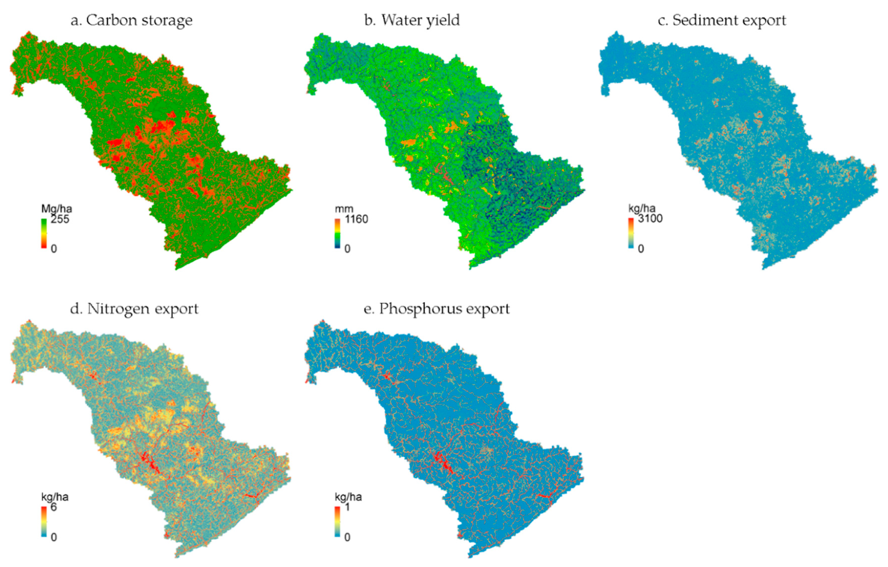
Figure 4.
Spatial distribution of modeled (a) carbon storage (mg per ha), (b) water yield (mm), (c) sediment export (kg per ha), (d) nitrogen export (kg per ha), and (e) phosphorus export (kg per ha) across the NFKR Watershed under the FRA scenario.
Figure 4.
Spatial distribution of modeled (a) carbon storage (mg per ha), (b) water yield (mm), (c) sediment export (kg per ha), (d) nitrogen export (kg per ha), and (e) phosphorus export (kg per ha) across the NFKR Watershed under the FRA scenario.

Table 1.
Ecosystem services assessed in this study and their biophysical indicators.
| Ecosystem Service | Biophysical Indicator | Unit | Description |
|---|---|---|---|
| Climate Regulation | Carbon storage | mg/ha | Average annual amount of carbon stored at each pixel |
| Flood Control | Water yield | mm | Annual water yield: low water yield indicating high flood control capacity |
| Soil Retention | Sediment export | Kg/ha | Annual average sediment export: low export indicating high retention capacity |
| Surface Water Quality | Nutrient (N and P) export | Kg/ha | The lower the N and P export, the better is the water quality |
Table 2.
Area of each land use land cover (LULC) type in 2001 and 2011 (unit, hectares) and its changes (unit, percent).
Table 2.
Area of each land use land cover (LULC) type in 2001 and 2011 (unit, hectares) and its changes (unit, percent).
| LULC | 2001 | 2011 | Change | Percent Change (%) |
|---|---|---|---|---|
| Water | 745 | 783 | 38 | 5.10 |
| Developed | 23,621 | 23,838 | 217 | 0.92 |
| Barren | 7923 | 11,767 | 3844 | 48.52 |
| Forest | 266,256 | 258,505 | −7751 | −2.91 |
| Shrub | 219 | 272 | 53 | 24.20 |
| Grassland | 39,011 | 42,533 | 3522 | 9.03 |
| Pasture | 5120 | 5196 | 76 | 1.48 |
| Total | 342,895 | 342,895 | 0 | 0 |
Table 3.
Size of area that has experienced transition from one land cover category to another between 2001 and 2011 (unit, hectares) in the North Fork Kentucky River (NFKR) watershed.
Table 3.
Size of area that has experienced transition from one land cover category to another between 2001 and 2011 (unit, hectares) in the North Fork Kentucky River (NFKR) watershed.
| 2011 | |||||||||
|---|---|---|---|---|---|---|---|---|---|
| 2001 | LULC | Water | Developed | Barren | Forest | Shrub | Grassland | Pasture | Total |
| Water | 720 | 1 | 11 | 4 | 0 | 9 | 0 | 745 | |
| Developed | 0 | 23,621 | 0 | 0 | 0 | 0 | 0 | 23,621 | |
| Barren | 27 | 16 | 5505 | 179 | 0 | 2189 | 7 | 7923 | |
| Forest | 14 | 97 | 4840 | 256,611 | 12 | 4594 | 88 | 266,256 | |
| Shrub | 0 | 0 | 9 | 6 | 198 | 6 | 1 | 219 | |
| Grassland | 2 | 96 | 1397 | 1705 | 62 | 35,726 | 2 | 39,011 | |
| Pasture | 0 | 6 | 5 | 1 | 0 | 9 | 5098 | 5120 | |
| Total | 783 | 23,838 | 11,767 | 258,505 | 272 | 42,533 | 5196 | 342,895 | |
The transition matrix shows the area of LULC that has transformed from one category to another (off-diagonal). The diagonal of the matrix shows size of area that did not change LULC between two time periods.
Table 4.
Mean production values of the five biophysical indicators of the ecosystem service by each land cover type under the 2011 LULC scenario. The standard deviation values are presented in the parenthesis after the mean production values.
Table 4.
Mean production values of the five biophysical indicators of the ecosystem service by each land cover type under the 2011 LULC scenario. The standard deviation values are presented in the parenthesis after the mean production values.
| LULC | Carbon Storage (mg per ha) | Water Yield (mm) | Sediment Export (kg per ha) | Nitrogen Export (kg per ha) | Phosphorus Export (kg per ha) |
|---|---|---|---|---|---|
| Developed | 28 (na) | 1055 (25) | 0.12 (0.21) | 4.34 (1.58) | 0.727 (0.264) |
| Barren | 0 (na) | 931 (21) | 971 (1921) | 2.00 (0.73) | 0.001 (0.001) |
| Forest | 250 (na) | 534 (84) | 110 (154) | 0.47 (0.25) | 0.003 (0.002) |
| Shrub | 100 (na) | 582 (79) | 122 (168) | 0.51 (0.24) | 0.003 (0.001) |
| Grassland | 45 (na) | 665 (69) | 404 (735) | 1.56 (0.65) | 0.020 (0.008) |
| Pasture | 51 (na) | 632 (51) | 628 (1205) | 1.59 (0.45) | 0.051 (0.015) |
Note: There is no variability in carbon storage within a land cover type calculated by the InVEST model. The sample size (i.e., number of cells) of each LULC class is the division of total area (as shown in Table 2) by cell size (0.01 ha).
Table 5.
Slope coefficient (Slope) and relative importance (RIMP) of the predictor variables estimated from a model average approach for explaining variability of the five biophysical indicators of ecosystem services at the subwatershed level.
Table 5.
Slope coefficient (Slope) and relative importance (RIMP) of the predictor variables estimated from a model average approach for explaining variability of the five biophysical indicators of ecosystem services at the subwatershed level.
| Predictor | Carbon | Water Yield | Sediment | Nitrogen | Phosphorous | |||||
|---|---|---|---|---|---|---|---|---|---|---|
| Slope | RIMP | Slope | RIMP | Slope | RIMP | Slope | RIMP | Slope | RIMP | |
| Forest | 1.00 ** | 1.00 | −0.29 ^ | 0.69 | −0.10 | 0.12 | −1.07 ** | 1.00 | −1.03 ** | 1.00 |
| STD_Forest | −0.02 | 0.11 | 0.21 | 0.37 | 0.12 | 0.14 | 0.19 | 0.08 | 0.09 | 0.07 |
| Elevation | 0.00 | 0.10 | −0.34 * | 0.59 | −0.07 | 0.11 | 0.26 * | 1.00 | 0.49 ** | 1.00 |
| STD_Elevation | <0.01 | 0.09 | −0.35 * | 0.49 | −0.06 | 0.10 | −0.14 | 0.19 | −0.38^ | 0.49 |
| Slope | <0.01 | 0.09 | 0.59 ** | 1.00 | 0.63 ** | 1.00 | 0.28 ** | 1.00 | 0.43 ** | 1.00 |
| STD_Slope | <0.01 | 0.10 | 0.47 ** | 1.00 | −0.03 | 0.10 | 0.07 | 0.12 | 0.28 ** | 1.00 |
| Precipitation | <0.01 | 0.09 | 0.83 ** | 1.00 | 0.20 | 0.45 | 0.11 | 0.58 | 0.11 | 0.27 |
| STD_Prep | <0.01 | 0.11 | 0.04 | 0.11 | 0.00 | 0.10 | −0.13 ^ | 0.59 | −0.20 ^ | 0.61 |
Note: Forest, STD_Forest are mean and standard deviation of forest land cover proportion within a subwatershed. Elevation and STD_Elevation are mean and standard deviation of elevation within a subwatershed. Slope and STD_Slope are mean and standard deviation of slope steepness. Precipitation and STD_Prep are mean and standard deviation of precipitation. The significance level was denoted with code ** p < 0.01, * p < 0.05, and ^ p < 0.1.
Table 6.
The modeled ecosystem service productions under the contemporary 2011 LULC condition and the FRA scenario and their differences.
Table 6.
The modeled ecosystem service productions under the contemporary 2011 LULC condition and the FRA scenario and their differences.
| Biophysical Indicators | 2011 LULC | FRA Scenario | Difference | Percent Change (%) |
|---|---|---|---|---|
| Carbon storage (mg C) | 71,343,168 | 80,633,377 | 9,290,209 | 13 |
| Water yield (mm) | 2219,528,435 | 2105,058,148 | −114,470,287 | −5.2 |
| Sediment export (kg) | 52,848,288 | 31,425,868 | −21,422,420 | −40.5 |
| Nitrogen export (kg) | 320,525 | 248,045 | −72,480 | −22.6 |
| Phosphorous export (kg) | 18,384 | 17,072 | −1312 | −7.1 |
© 2018 by the authors. Licensee MDPI, Basel, Switzerland. This article is an open access article distributed under the terms and conditions of the Creative Commons Attribution (CC BY) license (http://creativecommons.org/licenses/by/4.0/).
Share and Cite
MDPI and ACS Style
Gurung, K.; Yang, J.; Fang, L. Assessing Ecosystem Services from the Forestry-Based Reclamation of Surface Mined Areas in the North Fork of the Kentucky River Watershed. Forests 2018, 9, 652. https://doi.org/10.3390/f9100652
AMA Style
Gurung K, Yang J, Fang L. Assessing Ecosystem Services from the Forestry-Based Reclamation of Surface Mined Areas in the North Fork of the Kentucky River Watershed. Forests. 2018; 9(10):652. https://doi.org/10.3390/f9100652
Chicago/Turabian StyleGurung, Kumari, Jian Yang, and Lei Fang. 2018. "Assessing Ecosystem Services from the Forestry-Based Reclamation of Surface Mined Areas in the North Fork of the Kentucky River Watershed" Forests 9, no. 10: 652. https://doi.org/10.3390/f9100652
Note that from the first issue of 2016, this journal uses article numbers instead of page numbers. See further details here.