Predicting Tree Diameter Distributions from Airborne Laser Scanning, SPOT 5 Satellite, and Field Sample Data in the Perm Region, Russia

Abstract

A tree list is a list of trees in the area of interest containing, for example, the species, diameter, height, and stem volume of each tree. Tree lists can be used to derive various characteristics of the growing stock, and are therefore versatile and informative sources of data for several forest management purposes. Especially in heterogonous and unmanaged forest structures with multiple species, tree list estimates imputed from local reference field data can provide an alternative to mean value estimates of growing stock (e.g., basal area, total stem volume, mean tree diameter, mean tree height, and number of trees). In this study, reference field plots, airborne laser scanning (ALS) data, and SPOT 5 satellite (Satellite Pour l’Observation de la Terre) imagery were used for tree list imputation applying the k most similar neighbors (k-MSN) estimation method in the West Ural taiga region of the Russian Federation for diameter distribution estimation. In k-MSN, weighted average of k field reference plots with highest similarity between field reference plot and target (forest grid cell, or field plot) based on ALS and SPOT 5 features were used to predict the mean values of growing stock and tree lists for the target object simultaneously. Diameter distributions were then constructed from the predicted tree lists. The prediction of mean values and diameter distributions was tested in 18 independent validation plots of 0.25–0.5 ha in size, whose species specific diameter distributions were measured in the field and grouped into three functional groups (Pines, Spruce/Fir, Broadleaf Group), each containing several species. In terms of root mean squared error relative to mean of validation plots, the accuracy of estimation was 0.14 and 0.17 for basal area and total stem volume, respectively. Reynolds error index values and visual inspection showed encouraging results in evaluating the goodness-of-fit statistics of the estimated diameter distributions. Although estimation accuracy was worse for functional group mean values and diameter distributions, the results indicate that it is possible to predict diameter distributions in forests of the test area with the tested methodology and materials.

1. Introduction

Parameters describing tree diameter distribution (mean and standard deviation of diameter, shape of distribution) are commonly used in ecological and economic analysis in forestry. In ecological terms, varying size of trees have a clear influence on the dynamics of forest ecosystems [1]. The distribution of trees in forest stands in terms of their diameter at breast height (DBH) provides useful information for defining instructions for harvesting forest stands and for assessing the economic value of the size classes present [2,3].

Compartment level forest inventory information of the growing stock is very often presented as mean values. The mean values of parameters, such as basal area, total stem volume and stem count per ha, mean tree diameter, mean tree height, and forest age are listed by species and sometimes by age or canopy layer class (dominant, sub dominant, and under canopy trees). A more detailed way of presenting the information is to use tree size distributions or tree lists. A tree list is a list of trees in the area of interest containing, for example, the species, diameter, height and stem volume of each tree. Information in the tree list can be compressed in the form of tree size distributions where the frequencies of trees of similar size are presented. Tree lists are very versatile input data for various applications. For example, they can be used to derive mean values by species or by other classification as input data for applying tree level growth models or estimating amounts of timber sortiments in case of harvesting. Users of the inventory information can choose which trees are of interest and use the selected trees in further analysis. Field inventories aiming at producing tree lists or tree size distributions can be laborious, however the use of remotely sensed materials can drastically improve the efficiency of inventories. Airborne laser scanning (ALS) has been widely used in forest inventories and it has been proven to produce accurate inventory results that are comparable with field assessment methods (e.g., [4,5]). Accurate tree species mapping is challenging from ALS or from aerial optical data using automatic methods. For practical arrangements, species are grouped, for example, in three groups including separate classes for main coniferous tree species and all broadleaf species are described as one group (e.g., [4,5]). Inventory methods based on ALS can be roughly divided into two categories: area based approach (ABA) and detecting individual tree crowns (ITC); a third possible category is a mixture of ABA and ITC (for example [6,7,8]). It is possible to use ABA for estimating the mean values of the growing stock (for example [9,10,11]) or in the simultaneous estimation of mean values and tree lists (for example, [12,13]), while ITC always produces complete tree lists if all the trees are correctly detected (for example [14]).

Methods relying on ITC suffer from bias due to errors in tree crown detection, which are dependent on tree density and clustering [15]. Methods combining ITC and ABA do not suffer from bias due to errors in tree crown detection, however they still require the point density to be high enough to delineate individual trees. During the last decade, the ABA-based prediction of tree diameter distribution has become an optional procedure in forestry studies in Nordic countries [5]. There are several alternative ABA methods that are available to estimate tree lists or tree size distributions. Several studies have been complied regarding suitable distribution function, i.e., parametric (e.g., Weibull, beta, gamma, log-normal) and non-parametric (e.g., percentile prediction, k nearest neighbors) (see [16]) to choose independent and dependent variables and other parameters (number of nearest neighbors, plot sample size) [17]. Examples of ABA-based methods suitable for low point density data are:

• Tree list imputation using k-nearest neighbors (k-NN) methods (e.g., [12,13]).
• Direct estimation of parameters of theoretical distributions (for example [18]).
• Estimation of mean values and using existing models (parameter prediction) to estimate parameters of theoretical distributions (e.g., [12]).
• Estimation of mean values and parameters of theoretical distributions using parameter recovery [19,20].

It was demonstrated in [12] that Method 1 in the abovementioned list (tree list imputation) provides more accurate estimates of diameter distributions than Method 3 (parameter prediction). The k most similar neighbors (k-MSN) method was used to produce the estimates for tree lists and mean values. In [21], it was reported that parameter recovery, at its best, provided better accuracy for young stands and at least competitive accuracy for advanced stands when compared with existing distribution models used in Finland. Furthermore, [20] showed that parameter recovery method applied in ABA-based mean estimates is comparable to, or outperforms, comprehensive field measurements in estimating diameter distributions for the final cut stands.

Parametric estimation assumes that sample data comes from a population that follows a probability distribution that is based on a fixed set of parameters. In the case of forest structure estimation, parametric estimation is justified for homogenous single tree story layered stands. Conversely, non-parametric models differ in that the parameter set is not fixed and can increase, or even decrease if new relevant information is collected. There is no need to assume anything about the distribution, and we will rely only on the measurements. Non-parametric estimation is a safe strategy in heterogonous and unmanaged forest structures with multiple species [22]. Thus, the tree list imputation method can be considered to be a suitable initial method for Russian taiga conditions. This method can be used with low pulse density lidar data, which makes it cost efficient in large areas compared to ITC-based methods which require higher point density and are critical for the detection of individual tree crowns.

In Russia, traditional methods of analyzing and classifying forest stand structure are performed by age [23], while the concept of diameter distributions is not commonly used. According to [23], the main types of tree age structures based on tree distributions are:

• Relatively even-aged stands: The diameter distributions are unimodal and near normal.
• Absolutely uneven-aged stands: The diameter distributions are “negative-exponential” or “reverse J-shaped”.
• Relatively uneven-aged stands: The tree diameter distributions are multimodal, i.e., with several peaks.

Diameter distributions can, therefore, be used to describe the forest structure compatible with the traditional age-related classification. From the imputed tree list, the user of the inventory data can produce official reports with the required parameters, as well as compile information for forest management and timber procurement purposes. The method does not require existing models for predicting parameters for theoretical distributions and can be used in mixed species forests with multiple canopy layers. The downside of the tree list imputation method is that they require extensive and comprehensive field reference data for producing reliable estimates in forest areas with high variation in species mixture and forest structure.

This research is a continuation to previous research that was conducted by Kauranne et al. in 2017 [24], in which mean values were estimated within the same study area and materials, however with a different estimation method. As an independent study, the aim of this research is to test the imputation of tree lists with a k-MSN method in a taiga forest vegetation zone in the West Ural taiga region of the Russian Federation. Our research hypothesis is that k-MSN with tree list imputation can be used to describe all three main types of tree age structures based on tree distributions mentioned above (relatively even-aged stands, absolutely uneven-aged stands, and relatively uneven-aged stands). Additionally, the study area and materials make it possible to compare the estimation accuracies of mean values obtained with the sparse Bayesian regression [11] applied in the previous research and the k-MSN method applied in this research. We expect that k-MSN produces lower estimation errors for species group estimates, whereas sparse Bayesian regression performs better in the estimation of total mean values.

2. Materials and Methods

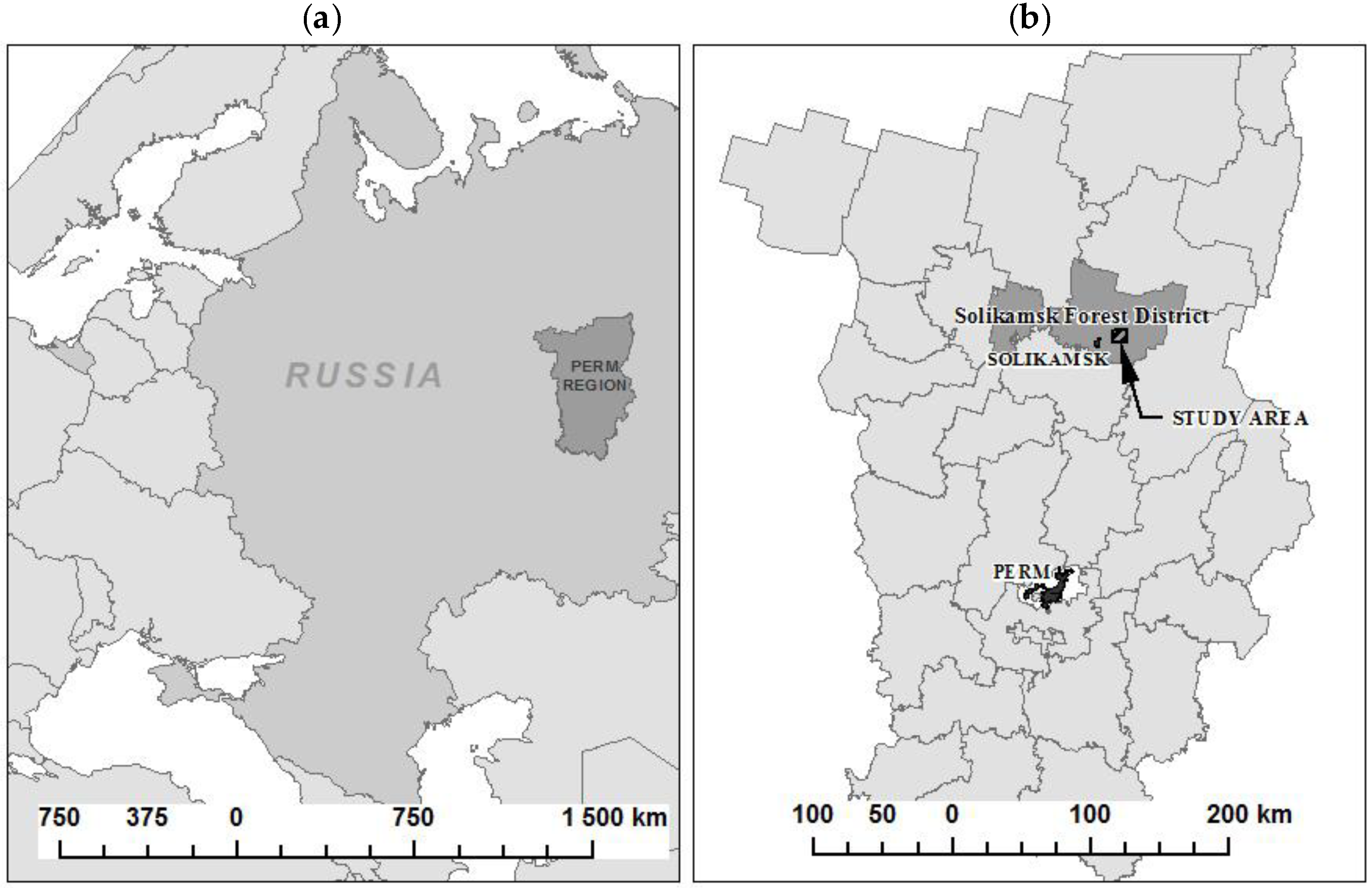
The materials are described in detail in [24], in which the same research data were used. The study area covers an area of 10 × 10 km, and it is located close to the village of Polovodovo, in the Solikamsk forest district, in the northern part of the Perm region, Russia (Figure 1).

The area of the Solikamsk forest district belongs to the taiga forest vegetation zone of the West Ural taiga region of the Russian Federation. The climate of the area is moderately continental, and the relief is mostly flat with hilly elevations. Two sub-regions are well recognized within the West Ural taiga region—one with a dominance of Nordic pine and spruce forests, and the other with a dominance of Kama-Pechora-Zapadnouralskih fir-spruce forests. Forests cover 85% of land area: Pine and spruce stands dominate in the study area, representing 42% and 34%, respectively, while birch and aspen stands occupy 20% and 4% of the forest stands, respectively.

The input data for the study included sparse point density ALS data, SPOT 5 (Satellite Pour l’Observation de la Terre) satellite images, field reference data, and field test data. ALS data were obtained in November 2013 with a Leica ALS70 CM LiDAR-scanner device (Leica Geosystems AG, Glattbrugg, Zurich, Switzerland). The resulting nominal pulse density at ground level was 3–4 points per square meter. ALS data were preprocessed by the data vendor, which included filtering and reclassifying into two classes such as ground and other points and transformation to las format in the WGS84 coordinate system. The ground classification was done with a triangulated irregular network (TIN)-based algorithm. The point cloud data using Terrasolid’s TerraScan software [25] were used for the data processing and for generating a digital terrain model (DTM) with 1-m pixel size. SPOT 5 high resolution satellite data were acquired on 7 August 2014. The preprocessing level of the imagery was 1A. The spatial resolution of the panchromatic band in the SPOT 5 images was 2.5 m, and 10 m for multispectral images. Geometric correction of the original imagery was performed using the ScanEx Image Processor software [26] and ground control points taken from aerial images that were collected during the same flight with lidar acquisition. The resulting spatial resolution of the geometrically corrected images was 10.7 and 2.7 m for multispectral and pan-sharpened images, respectively.

A total of 281 9-m radius circular field reference plots were used as training data. Plots were sampled in four plots per cluster with 200 m distance between the plots in one cluster. The aim of the sampling was to obtain a representative sample of all forest types and development stages (young, developing, mature) in the whole inventory area. Forest type information from an existing stand database and ALS heights were used as a priori information in sampling to distribute reference plots in forest types and development stages. The sampling design follows the sampling that was used in Finland by Finnish Forest Centre for ALS-based forest inventory campaigns [27] with adjustments for the available data. The sampling design used in this research is presented in detail in [24]. Initially, 308 plots were measured in the field between summer 2015 and autumn 2016. DBH, tree class (dead or alive), and species was recorded for each tree with a DBH value of at least 6 cm. Heights were measured for height sample trees (maximum of three for every species in a plot) and the heights for the rest of the trees were estimated using a diameter-height (d-h) curve estimated from the height sample tree data. Volumes were then estimated for all trees by applying local volume tables. The calculation process is described in detail in [24]. The process produced a complete tree list for every field plot, including species, tree class, DBH, height, and stem volume for every standing tree with a DBH value of at least 6 cm. Species were classified into three functional groups—Pines (Pinus sylvestris L. and Pinus sibirica Du Tour), Spruce/Fir (Picea abies Karst. and Abies sibirica Ledeb.), and Broadleaf Group (Betula pendula Roth, Tilia cordata Mill., Populus tremula L., Salix caprea L., and Alnus incana L.)—and total stem volume per ha (V), basal area (G), number of stems per ha (N), and basal area weighted mean diameter (D) and height (H) were calculated for totals and for functional groups from the tree list. Twenty-seven of the original 308 plots were removed because they were either outside ALS data coverage, over 60% of plot’s total volume was from standing dead trees, the field-measured data was unrealistic and not logical, or it was considered to be highly plausible that there were problems in matching the field data with the ALS data. The last analysis was based on comparing field-measured mean tree height and ALS height; if the difference between field-measured mean tree height and the 90% percentile of ALS height was over five meters, the plot was removed. Statistics of the 281 field reference plots are presented in

Table 1. Field reference plot statistics and mean values, with standard deviations in parentheses. n = 281.

Variable	Pines	Spruce/Fir	Broadleaf Group	Total
Total stem volume (m3 ha−1)	151.1 (159.6)	142.7 (141.1)	68.0 (113.0)	361.7 (163.3)
Basal area (m2 ha−1)	14.4 (14.6)	15.0 (13.1)	6.9 (10.6)	36.3 (14.0)
Number of stems (n ha−1)	317.0 (409.7)	618.5 (428.7)	244.1 (380.7)	1180.0 (533.0)
Basal area weighted mean height (m)	21.7 (4.3)	16.6 (5.6)	18.4 (5.2)	20.4 (3.6)
Basal area weighted mean diameter (cm)	28.9 (8.2)	21.2 (8.8)	21.5 (8.8)	26.2 (6.1)

.

Independent test data consisted of 18 rectangular control plots that were established in the study area. The plots were laid in the middle part of a forest stand in selected stands representing typical mature forests of the study area. The location of each plot was recorded using Global Positioning System (GPS) handheld devices. The plot sizes varied from 0.25 to 0.5 ha. Diameters were measured in 4-cm diameter classes for all trees with a minimum DBH value of 6 cm. Heights were measured for height sample trees and volumes were calculated based on local volume tables. The mean values were then calculated for totals and for functional groups. Based on functional group containing most of the total volume, the test plots represent functional groups, as follows: 12 plots in Pines, five plots in Spruce/Fir, and one plot in Broadleaf Group. All of the plots were in mixed stands comprising species at least from two functional groups. Pines and Spruce/Fir occurred in all plots and Broadleaf Group in six plots. The measurement protocol differs from the protocol used with field reference plot data, and did not produce tree list information or accurate estimates for H and D. Statistics of the field test plots are presented in

Table 2. Field test data statistics and mean values, with standard deviations in parentheses. n = 18.

Variable	Pines	Spruce/Fir	Broadleaf Group	Total
Total stem volume (m3 ha−1)	276.4 (159.0)	147.3 (143.2)	35.7 (130.5)	459.4 (131.7)
Basal area (m2 ha−1)	23.1 (12.6)	13.5 (11.8)	2.9 (10.3)	39.5 (9.8)
Number of stems (n ha−1)	419.8 (267.3)	407.6 (253.0)	34.1 (104.9)	861.5 (252.1)

.

A k-MSN model for the simultaneous estimation of mean variables and tree list imputation was formulated based on 281 reference plots. The ALS variables, based on features described in [28], were calculated for the plots from the height-normalized ALS point cloud. The ALS variables include height percentiles for the first-pulse and last-pulse returns, mean height of first-pulse returns above 5 m (high-vegetation returns), standard deviation for first-pulse returns, the ratio between first-pulse returns from below 2 m and all first-pulse returns and the ratio between last-pulse returns from below 2 m and all last-pulse returns. Linearizing transformations of the ALS variables were also calculated. From SPOT 5 data, the mean values from each band were calculated, as well as mean values from band combinations calculated as: (band a − band b)/(band a + band b). The band combinations used were bands 1 and 2, bands 3 and 2, and bands 1 and 3. The ArboLiDAR software package [29] was used for the calculation of independent features and the estimation of k-MSN model. All ALS and SPOT 5 variables are described in Table S1.

K-MSN is a non-parametric estimation method which uses the canonical correlation analysis to produce the weighting matrix for selecting k most similar neighbors from reference plots in terms of independent (predictor) variables. Through canonical correlations, it is possible to find the linear transformations U_k and V_k, for the set of dependent variables Y and independent variables X, which maximize the correlations between them:

$$U_k={\alpha }_{k}Y \mathrm{and} V_k={\mathsf{\gamma }}_{k}X$$

(1)

where α_k are the canonical coefficients of dependent variables and γ_k are the canonical coefficients of the independent variables (k = 1, …, s). The most similar neighbors (MSN) distance metric between plot u and plot j derived from canonical correlation analysis is described, as follows [30]:

$$D_{uj}^2=\begin{array}{c}\left(X_u-X_j\right)\\ 1\times p\end{array}\begin{array}{c}\Gamma {Ʌ}^2{\Gamma }^{\prime }\\ p\times p\end{array}\begin{array}{c}{\left(X_u-X_j\right)}^{\prime }\\ p\times 1\end{array}$$

(2)

where X_u is the vector of independent variables from target observation, X_j is the vector of independent variables from the reference observation, Γ is the matrix of canonical coefficients of the independent variables, and Ʌ is the diagonal matrix of squared canonical correlations.

In the case of k > 1, the estimates were calculated as weighted averages of k-MSN using inverse of MSN distances:

$$W_{uj}=\frac{\left(\frac{1}{1+D_{uj}^2}\right)}{{\sum }_{i=1}^k\left(\frac{1}{1+D_{uj}^2}\right)}$$

(3)

where $D_{uj}^2$ is the MSN distance for target plot u of the reference plot j.

Variable selection for k-MSN estimator was done in two phases. First, the initial set of independent variables was taken from [24], in which the variables were used in sparse Bayesian estimator. Then, variables and value of k were tested manually with the k-MSN method and they were evaluated via the relative root-mean-squared errors (RMSE) of V, G, N, H, D, and volumes of functional groups. RMSE was calculated, as follows:

$$\mathrm{RMSE}=\sqrt{\frac{{\sum }_{i=1}^n{(y_i-{\widehat{y}}_i)}^2}{n}}$$

(4)

where $y_i$ is the observed value, ${\widehat{y}}_i$ is the estimated value for the reference plot i, and n is the total number of reference plots. RMSEs were calculated relative to the mean, i.e., the value from Equation (4) was divided by the mean of the observed value. Effect of the parameter k was tested manually with the selected set of independent variables. Value of k was increased until the RMSE of the estimated G, N, V, or D stopped improving. G, N, V, and D were used because they have a strong correlation with diameter distributions [31].

Leave-one-out cross-validation (LOOCV) was used in model validation process for reference plot data. After the optimal value for k and independent variables were found in reference plot data, the model was tested in test plot data. The estimates for test plots were calculated through a grid approach, i.e., the plot was divided into grid cells whose sizes corresponded to the area of a reference plot, estimates were imputed for the cells and cell level estimates were aggregated at the test plot level. The estimated and observed results were then compared using RMSEs.

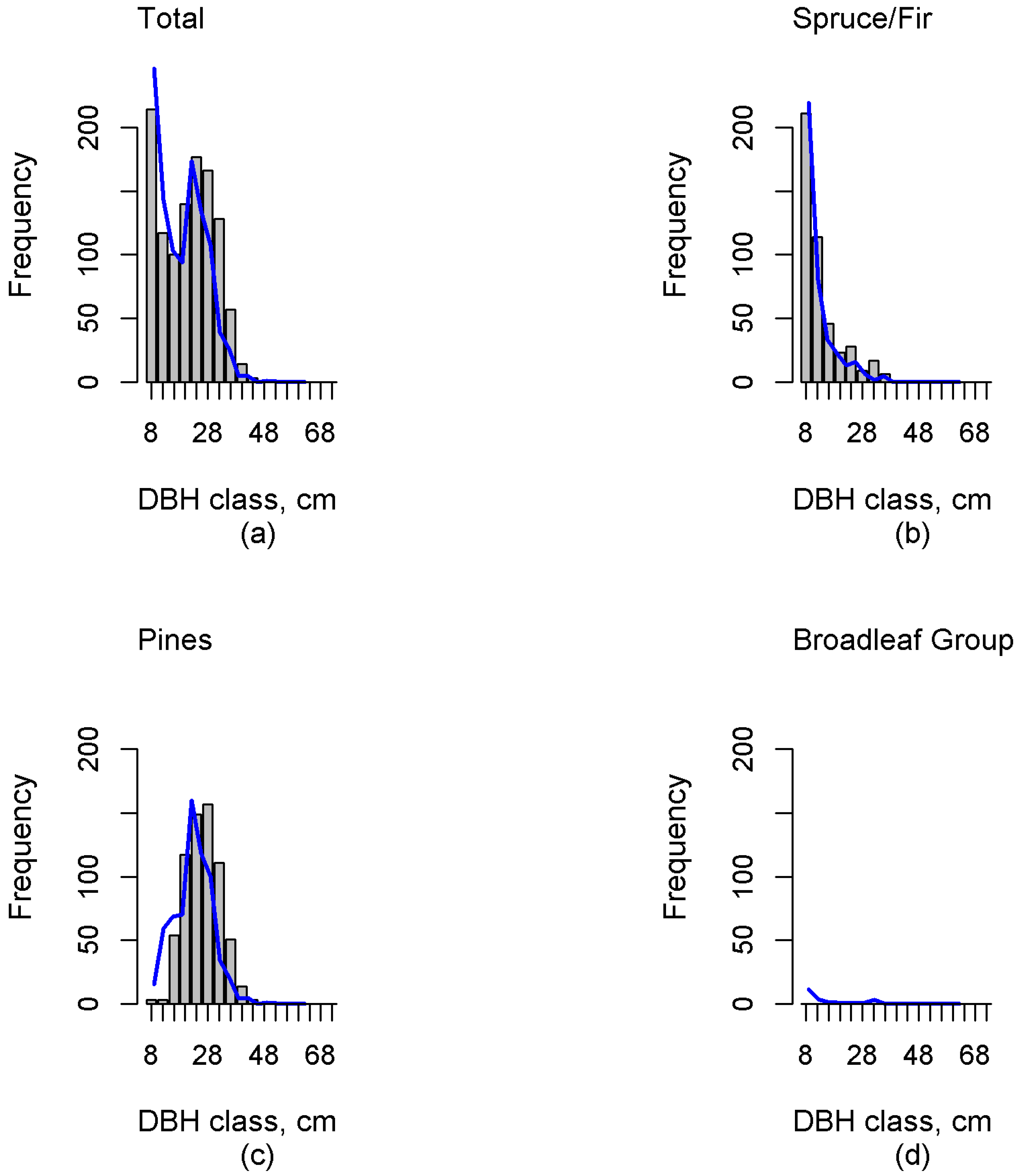
Additionally, tree lists were imputed with the k-MSN method for each grid cell of the test plots. Cell level tree lists were aggregated to test plot level and binned into diameter classes with 4-cm intervals. The value of each bin represented the stem count of trees in that diameter class. This produced diameter distribution with frequencies that were proportional to the number of stems. Diameter distributions were aggregated for the total number of trees and separately for every functional group.

To compare the estimated and observed distributions in each test plot, the Reynolds error index [32] was calculated in a similar way, as in [31], for all the diameter classes and for diameter classes that include only trees larger than 22 cm at breast height (Equation (5)).

$$e=\frac{{\sum }_{i=1}^m\left|n_{pi}-n_{oi}\right|}{N} 100$$

(5)

where $n_{pi}$ and $n_{oi}$ are the imputed and observed number of trees per ha in diameter class i and $N$ is the total number of trees per ha of observed test plot measurements.

3. Results

The results are presented within the reference data (for mean values only) and in independent test data. The reference data validation allows for the comparison of the k-MSN estimates with the sparse Bayesian estimates. In independent test data, the main emphasis is on the investigation of diameter distributions.

3.1. Validation within Reference Data

The prediction model was tested with several values of k and set of independent variables. Here, we present the validation results with the optimal parameter values found in reference plot data. The optimal value found for k was 6. The number of independent variables used in the model was 14, including 11 variables derived from ALS data and three variables from SPOT 5 data (see Table S1 for selected variables). Five of the ALS variables were height percentiles, five variables described density at different relative or absolute heights and one variable was calculated as a product of height and density variable. SPOT 5 variables included mean values from band combinations 3 and 2 from multi-spectral and multi-spectral pan-sharpened images and mean of green band. Plot-level validation results are presented in Figure 2 with the validation results from the sparse Bayesian model that is presented in [24]. Based on plot level LOOCV and RMSE values, sparse Bayesian performed better than or equally well to the estimation of all but four parameters. K-MSN performed better for N, H, and D of Broadleaf Group, and for H of Spruce/Fir group. For most of the estimated parameters (12/20), the difference was smaller than three percentage units and for 18/20 it was less than seven percentage units. The largest differences (about 15 percentage units) in favor of sparse Bayesian were in H and D of Pines.

3.2. Validation within Independent Test Data

Based on the 18 independent test plots, the error and bias were small. There was no significant bias in the G estimates, however there was significant bias in estimates of N for all functional groups, except Pines (

Table 3. The RMSE (relative root-mean-squared errors) values and biases relative to mean of test plots (n = 18).

Variable	Pines		Spruce/Fir		Broadleaf Group		Total
	RMSE	Bias	RMSE	Bias	RMSE	Bias	RMSE	Bias
Total stem volume	0.32	0.13	0.59	0.03	1.19	0.09	0.17	0.09 *
Basal area	0.30	0.02	0.53	−0.10	0.97	−0.09	0.14	−0.03
Number of stems	0.41	−0.02	0.72	−0.52 **	2.33	−1.73 **	0.45	−0.32 **

Biases marked with * are statistically significant with risk level 0.05, and biases marked with ** are statistically significant with risk level 0.01.

). Removing small trees from the test plot data improved both the error and bias of N but increased the error of G in Spruce/Fir and Broadleaf Group (

Table 4. The RMSE values and biases relative to mean of test plots considering only trees with a minimum value of diameter at breast height (DBH) of 22 cm (n = 18).

Variable	Pines		Spruce/Fir		Broadleaf Group		Total
	RMSE	Bias	RMSE	Bias	RMSE	Bias	RMSE	Bias
Basal area	0.31	0.03	0.62	0.03	1.33	0.17	0.15	0.04
Number of stems	0.32	0.05	0.60	0.07	0.40	−0.22 *	0.13	0.04

Biases marked with * are statistically significant with risk level 0.05. Biases marked with ** are statistically significant with risk level 0.01.

). Ref. [24] reported RMSEs relative to the mean for V of 0.14 and 0.13 in 0.25 and 0.5 ha validation data, respectively. These are smaller values than that which we present here for k-MSN. In [24], the calculated RMSEs relative to the mean for G were 0.16 and 0.12 in the 0.25 and 0.5 ha validation data, respectively. These are at similar level with the value that was obtained in our results.

Estimates of diameter distributions were successfully produced for distributions of different shape. Distributions were investigated visually and by using Reynolds error index (

Table 5. The mean, minimum and maximum Reynolds error index values of test plots for diameter distributions including all diameter classes and diameter classes with a minimum DBH value of 22 cm.

Statistics	Pines		Spruce/Fir		Broadleaf Group		Total
	All	Min 22	All	Min 22	All	Min 22	All	Min 22
Mean	28.20	15.17	48.91	10.74	10.15	2.67	66.57	15.71
Minimum	8.15	5.06	8.75	1.26	1.60	0.00	17.99	8.33
Maximum	46.74	28.91	97.96	26.95	52.34	24.95	122.94	27.13

). Figure 3, Figure 4 and Figure 5 show examples of the best, the average, and the worst agreement between estimated and measured distributions, according to the Reynolds error index. The order from best to worst was decided by summing up the Reynolds error index values of functional group and total distributions using all diameter classes. Reynolds error index values and visual inspection of goodness-of-fit seem to be congruent. As shown in Figure 3, the proportions of functional groups and the shape of the estimated distributions seems to fit well in the measured data. In Figure 4, representing an average goodness-of-fit, there is mixing of Pines and Spruce/Fir groups and the lower end of Spruce/Fir distribution is poorly estimated. This is typical for estimates: the estimated Spruce/Fir distributions are always skewed right, having a high proportion of trees in the smallest diameter classes. Figure 5 represents the worst goodness-of-fit. The distribution has wrong shape and the number of trees in Pines and Broadleaf Group are overestimated.

4. Discussion

In this study, we tested the prediction of tree diameter distributions using the tree list imputation method and ALS data for all DBH classes at the plot and the stand level in a temperate forest in Russia. Our results indicate that it is feasible to predict diameter distributions in Russian forests on the basis of sparse ALS data. 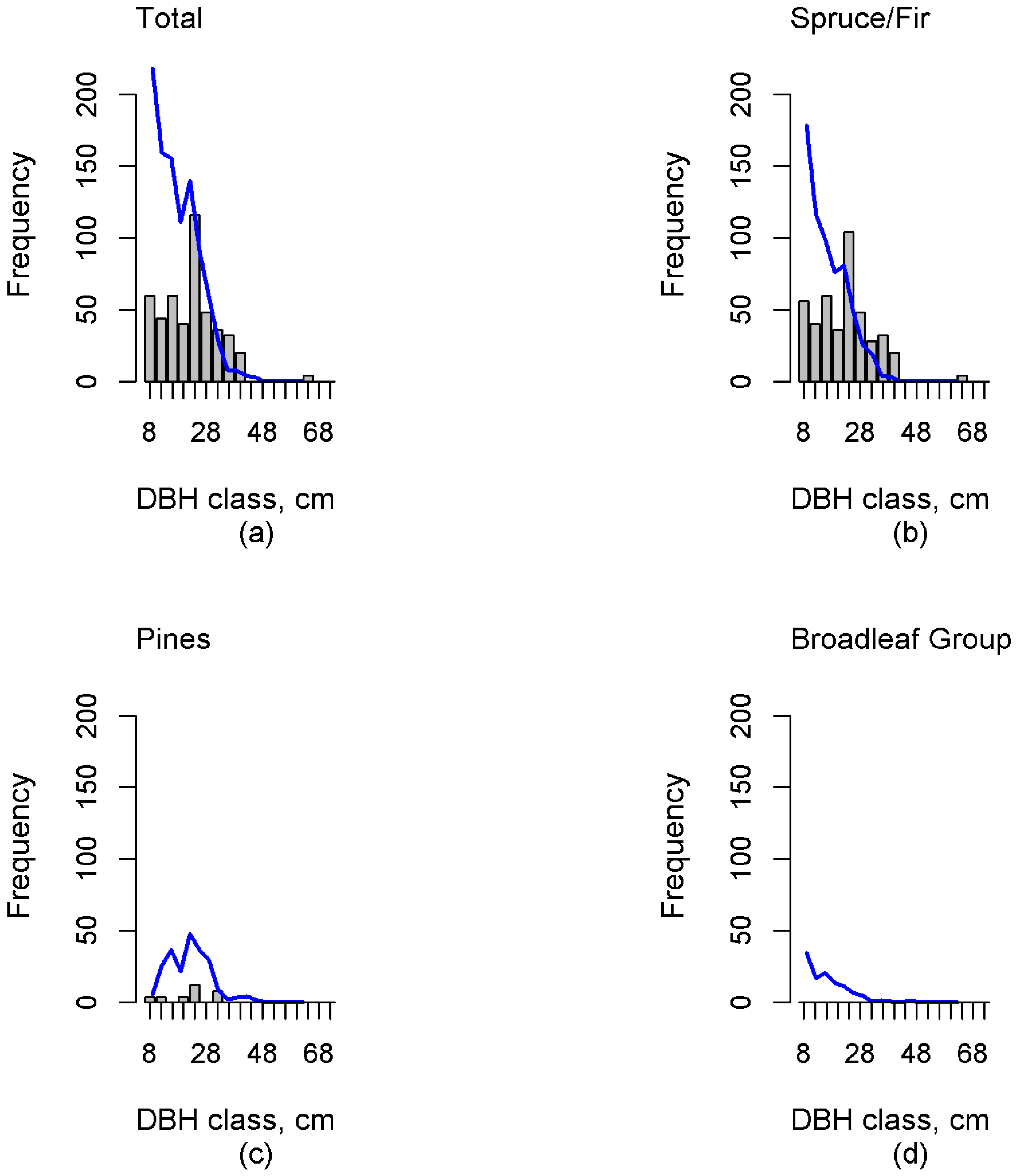Due to the lower costs of acquiring sparse ALS data, and its higher accuracy for predicting the frequencies of all diameter classes, diameter distribution modelling can offer a comparable alternative to methods that are based on individual tree detection [33]. We were able to estimate unimodal, negative exponential, and multimodal distributions at functional group level. Validation in independent test data showed that diameter classes containing larger trees (DBH values over 22 cm) were, in general, more accurately estimated than diameter classes of smaller trees (spruce, fir and deciduous trees belonging to the under canopy). 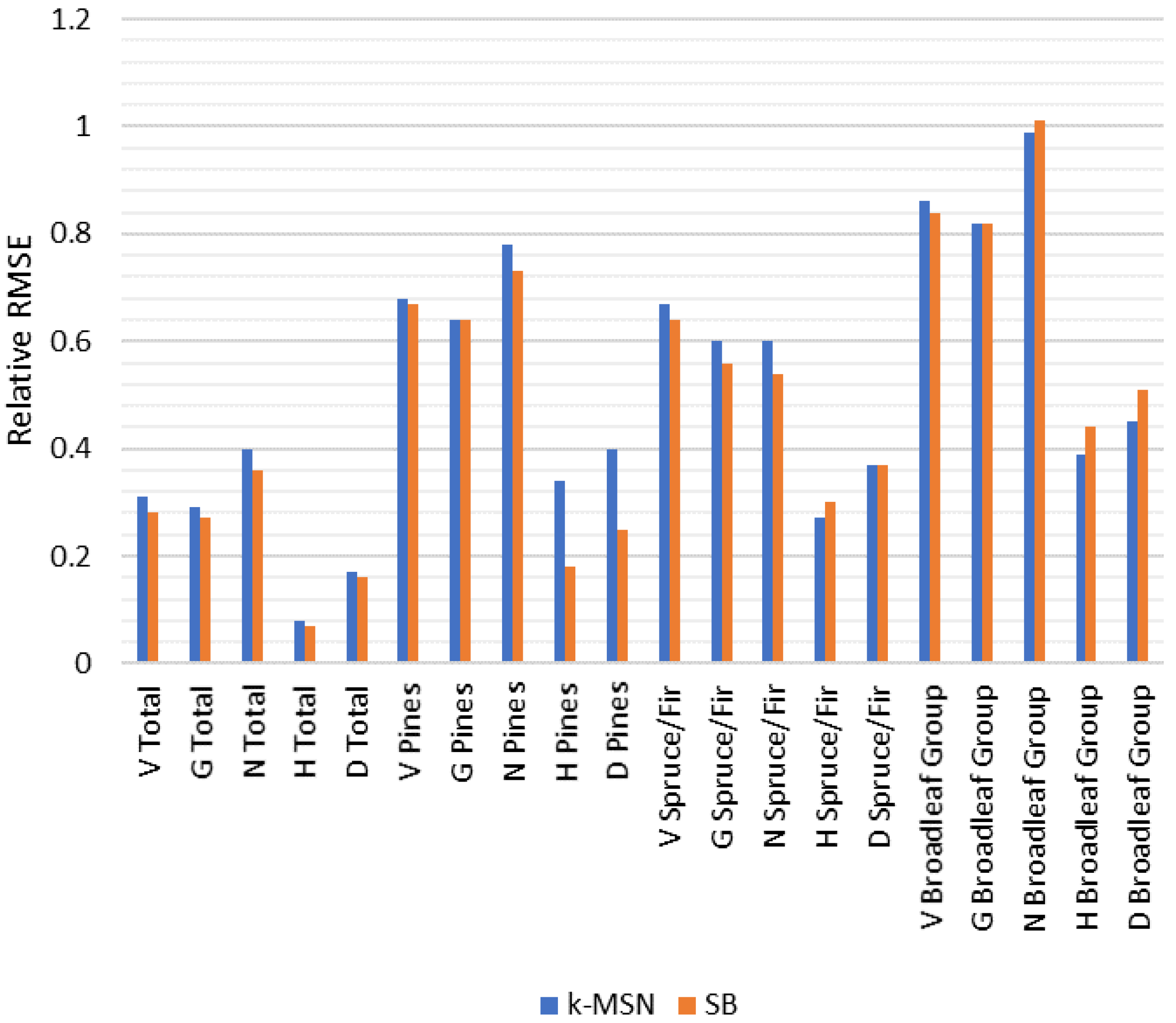Comparison with results of an earlier study [24] indicated that mean variables could be estimated with better accuracy using sparse Bayesian than they could with k-MSN with the used reference field data, including most of the functional group level results.

The choice of dependent variables and independent predictors plays a crucial role in determining the k-NN based diameter distribution when using ALS data. The choice of dependent variables and independent predictors was assessed via the RMSE% of the mean values, which contributed the most weight in G, N, V, and D, which suggested the goodness-of-fit of the estimated diameter distribution. The selection of dependent variables and independent predictors by means of minimization of RMSE is common to many studies, such as [16,17,34,35]. We used V, N, and G as dependent variables, as were done in [17,31], as well as D. These dependent variables were sufficient to describe the structure of the diameter distribution in our estimation process. The number of independent variables in our k-MSN model was 14. In [17], it was recommended that number of independent variables should be kept low to avoid the over-fitting of the model in reference data. A higher number of independent variables can produce lower RMSE values in LOOCV, however with independent test data, or in a prediction situation, a model with a lower number of independent variables may perform better. In the end, 12 independent variables derived from ALS data were used in [17] to estimate total mean values and diameter distributions. In our study, we estimated functional group parameters and used satellite features in addition to ALS features. Thus, the final number of ALS (11) and SPOT 5 (3) features used as independent variables is well consistent with the recommendation that is given in [17].

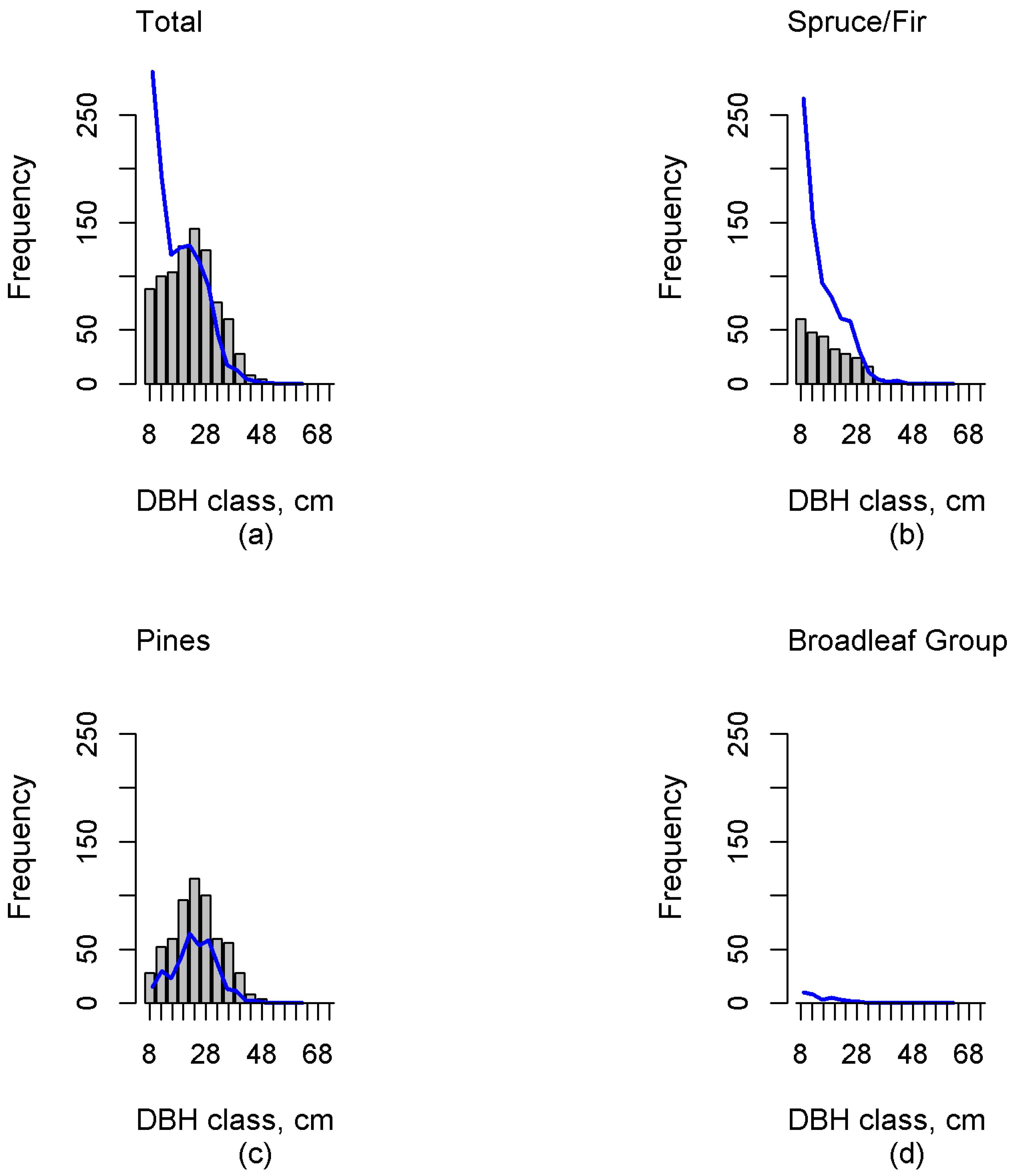
Investigation of the errors revealed possible deficiencies in the reference plot data. The sample dataset should contain the entire variability in forest characteristics, including dominant and suppressed tree features (e.g., density, height, volume), and consequently this inclusion in the training set will ensure a reasonable estimation accuracy. Independent validation data plays a crucial role in result validation. Our results in independent test data showed that this study was able to estimate multimodal distributions. Additionally, the proportions of functional groups were, in general, well estimated. However, in the case of the Spruce/Fir the diameter distribution estimates were skewed right (“reverse J-shaped”), which was not always congruent with the field-measured distribution. This can clearly be seen, for example, in Figure 3, Figure 4 and Figure 5. Additionally, including all DBH classes estimates of N were biased for all but the Pines. When including only trees with a minimum DBH value of 22 cm, the biases reduced, and only the bias of the Broadleaf Group was significant. The total volume estimate was underestimated by 9% in whole data. For larger diameter classes, G and N were also underestimated, although based on t-test the bias was insignificant. The results indicate that there were potential problems in describing the amount of small, suppressed trees in mature forests, and in describing the amount of the largest trees. In the test plot data, this results in systematic overestimation of the number of small trees and the possible underestimation of the number of large trees. To summarize for reference plot data, sample size could be increased to better capture the variability in absence or occurrence of smaller trees and the largest trees.

Comparison of k-MSN and sparse Bayesian showed noticeable differences between the methods. When compared with an earlier study [24], estimation errors were smaller with the sparse Bayesian method, including estimates for functional groups; the only exceptions in favor of k-MSN were variables describing tree size in Spruce/Fir and Broadleaf Group. Trees in Spruce/Fir and Broadleaf Group were, on average, smaller than trees in Pines, and especially trees in Spruce/Fir often presented lower canopy layer, i.e., under canopy trees. In our data, the Broadleaf Group presented more rare cases, i.e., minor species. This could indicate that k-MSN is better suited in situations where the interest is in describing the structure of forest, including all canopy layers and minor species, whereas sparse Bayesian can be more efficient if total mean values are the main interest. Another reason for these results could be that in the present study there was a quite limited number of field reference plots, which may not have been enough to cover the variation of forest characteristics for the k-MSN method in the study area.

Accurate remote sensing of tree species has varied with stand heterogeneity. In passive optical remote sensing, radiance information from forest canopies has been used to distinguish tree species. Although the main tree species and homogeneous stands are predicted well, the error in the heterogeneous stands and for minor tree species can be very high [5]. Widely used photogrammetric multispectral sensors include the Vexcel UltraCam-D (Vexcel Imaging, Graz, Austria), the Intergraph-Z/I (Intergraph, Huntsville, AL, USA), and the Leica ADS40 (Leica Geosystems AG, Glattbrugg, Zurich, Switzerland). These sensors have been used in single-tree species classification and analysis (e.g., [36,37,38,39]). In these studies, classification accuracies of 80%–93% were reported for Scots pine, Norway spruce, and birch (Betula pendula and Betula pubescens Ehrh.). In this study, we obtained similar accuracy, although the dataset was rather small. In ABA, fusing ALS data with auxiliary optical data improves species estimation significantly when compared with using ALS data only [40]. In [40], it was demonstrated that, while aerial images performed the best individual material in species estimation, the combination of all tested auxiliary data—i.e., aerial images, Sentinel-2 and Landsat 8 images—gave even better species estimates. Thus, the results we presented here for the functional group proportions can be improved by fusing optical data from other satellite and aerial imaging systems.

5. Conclusions

Diameter distributions and mean values of growing stock were estimated fusing field reference data, optical satellite data and ALS data in k-MSN estimation framework in Perm region, Russia. The estimation was successful in describing heterogenous structure of forests and multimodal distributions. However, the applied method with the available data was not able to capture the features of under canopy layer correctly. In general, the accuracy of mean value estimation was worse than with alternative method, sparse Bayesian regression, applied in earlier study. Albeit, the differences between RMSEs were small and for some mean values (variables describing mean tree size of under canopy trees or minor species) k-MSN produced more accurate results. The results obtained demonstrate that ALS-based systems fusing carefully measured field reference data and auxiliary optical data can be considered as alternatives to the commonly used field plot-based forest inventory, with preconditions considering species mapping. It is not feasible to map all species accurately with the method, and therefore, some grouping of species is required, and accurate estimates can be produced only for the main species. This means that it is possible to partly replace field work by ALS remote sensing and thus improve forest structure mapping methods. However, careful field control mechanisms are required for heterogenous forests and in case of mapping several species accurately. Future research and development is required to adjust methods for better describing under canopy layer and tree species proportions.