Landscape Transformation under Global Environmental Change in Mediterranean Mountains: Agrarian Lands as a Guarantee for Maintaining Their Multifunctionality


Abstract
:1. Introduction
2. Materials and Methods
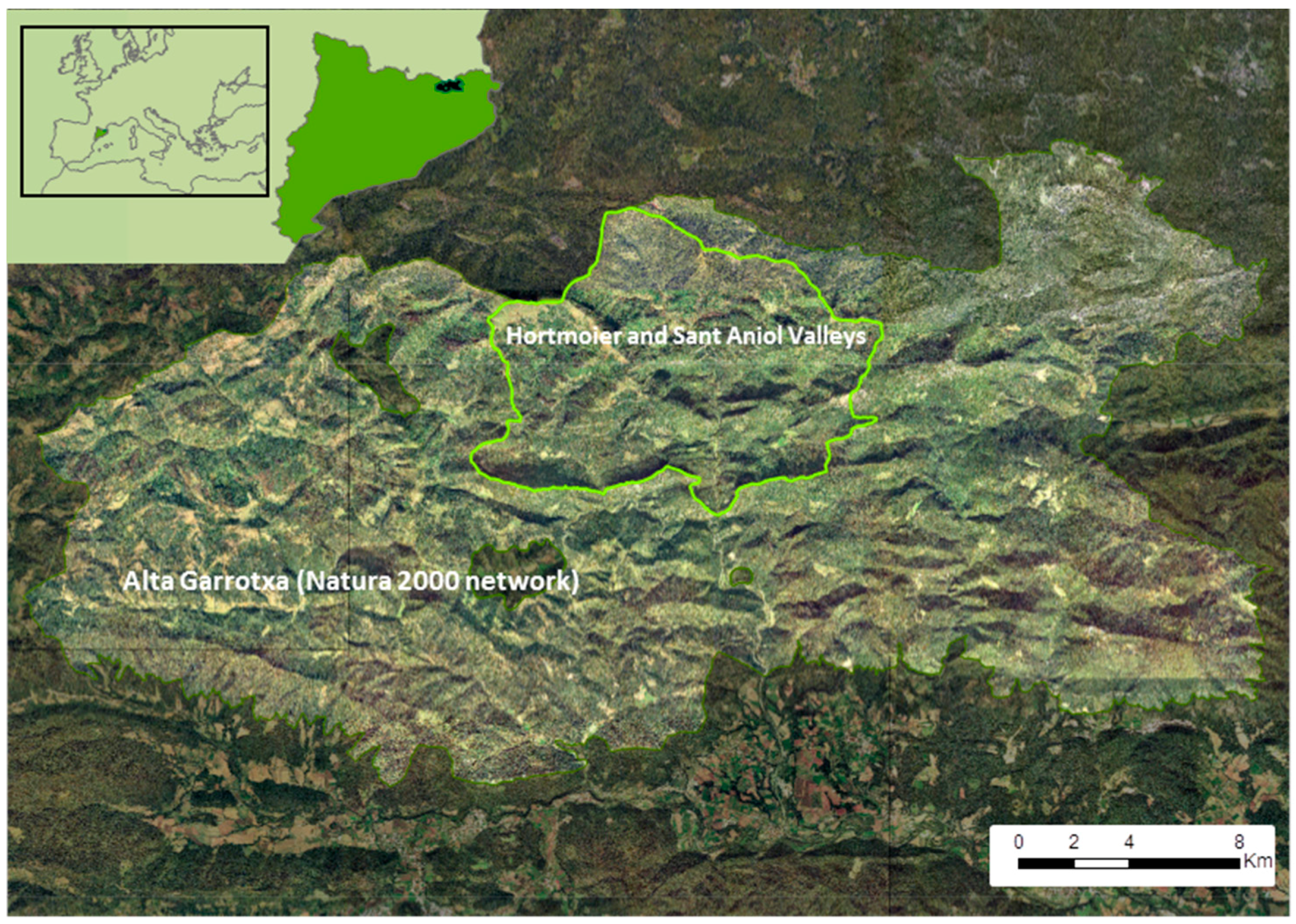
2.1. Study Area
2.2. Composition and Landscape Configuration
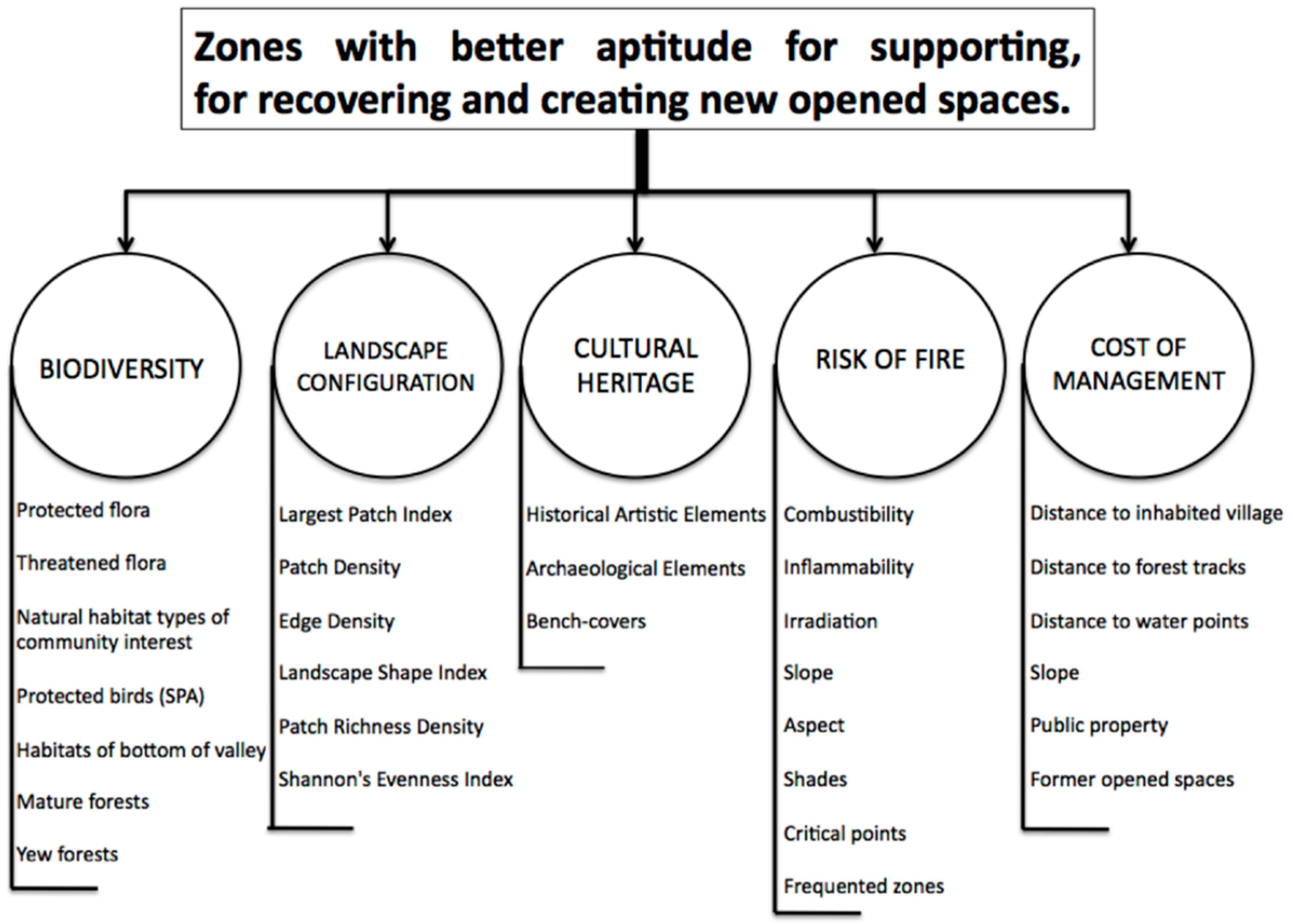
2.3. Creating New Agrarian Spaces Using Multi-Criteria Analysis and Geographic Information Systems (GIS)
3. Results
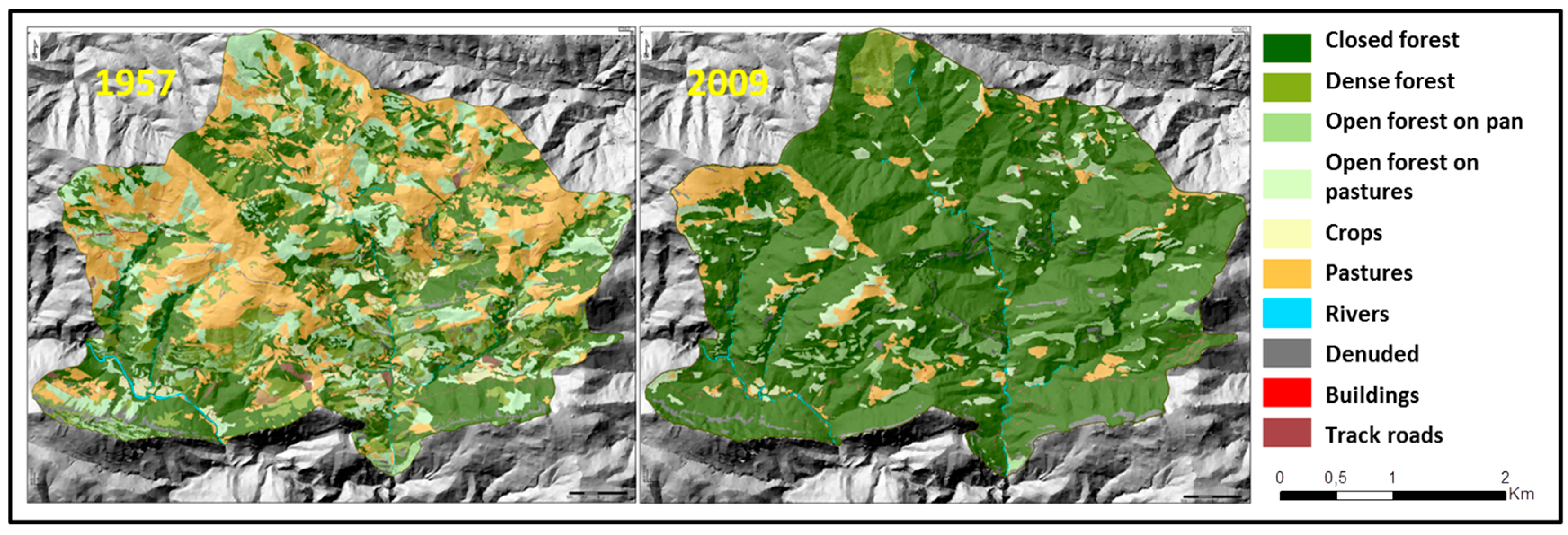
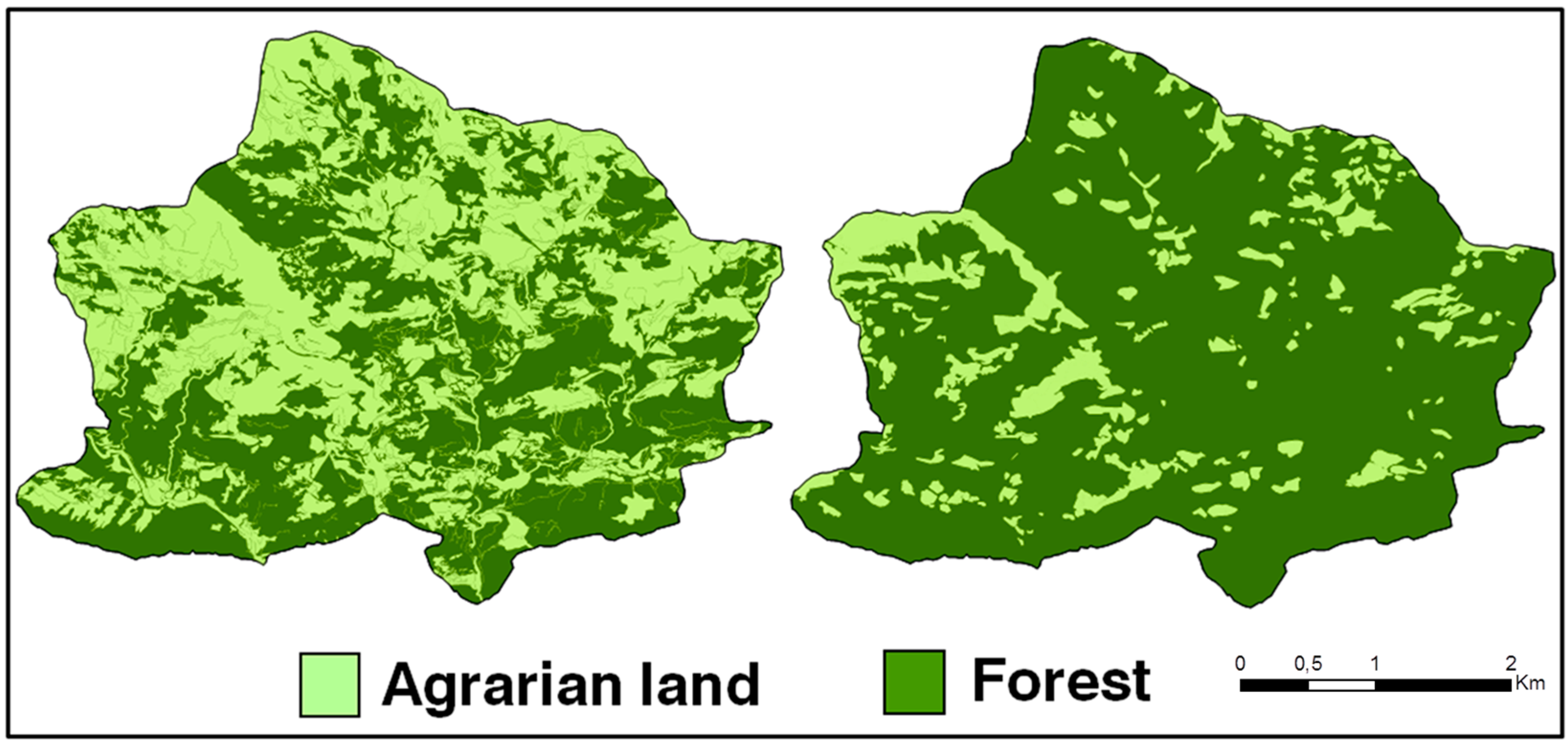
3.1. Landscape Composition Changes Over the Last Fifty Years
3.2. Landscape Configuration Changes Over the Last Fifty years
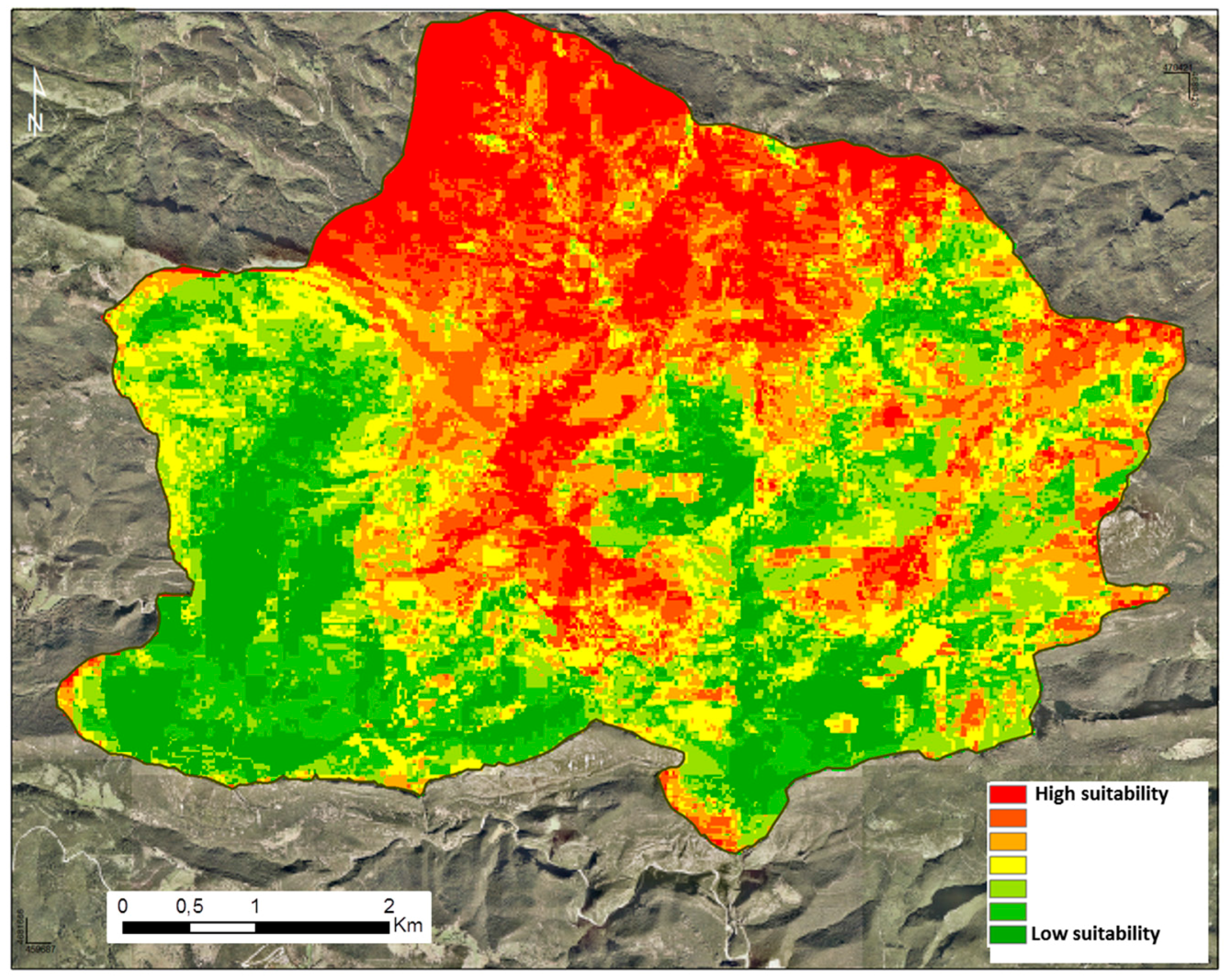
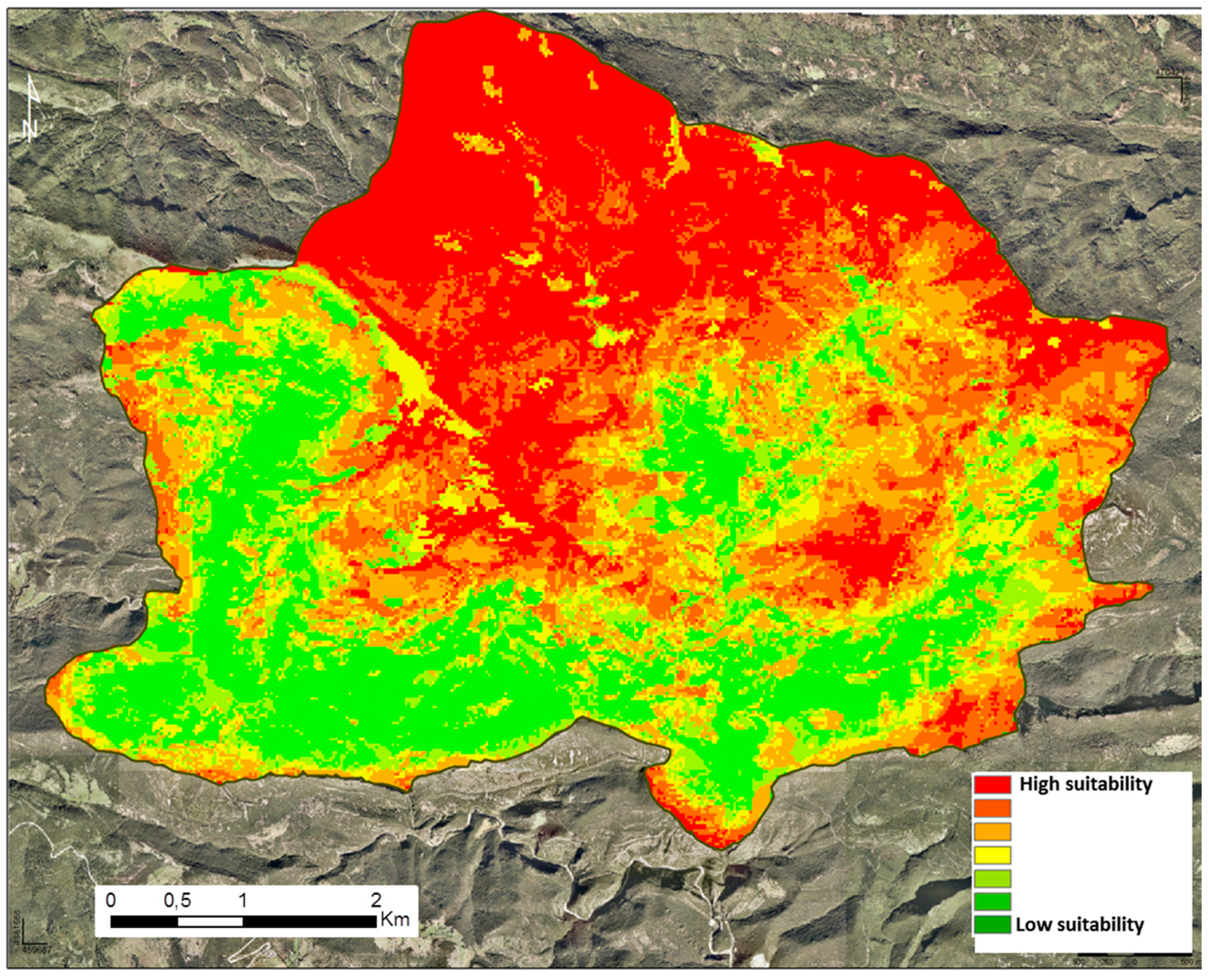
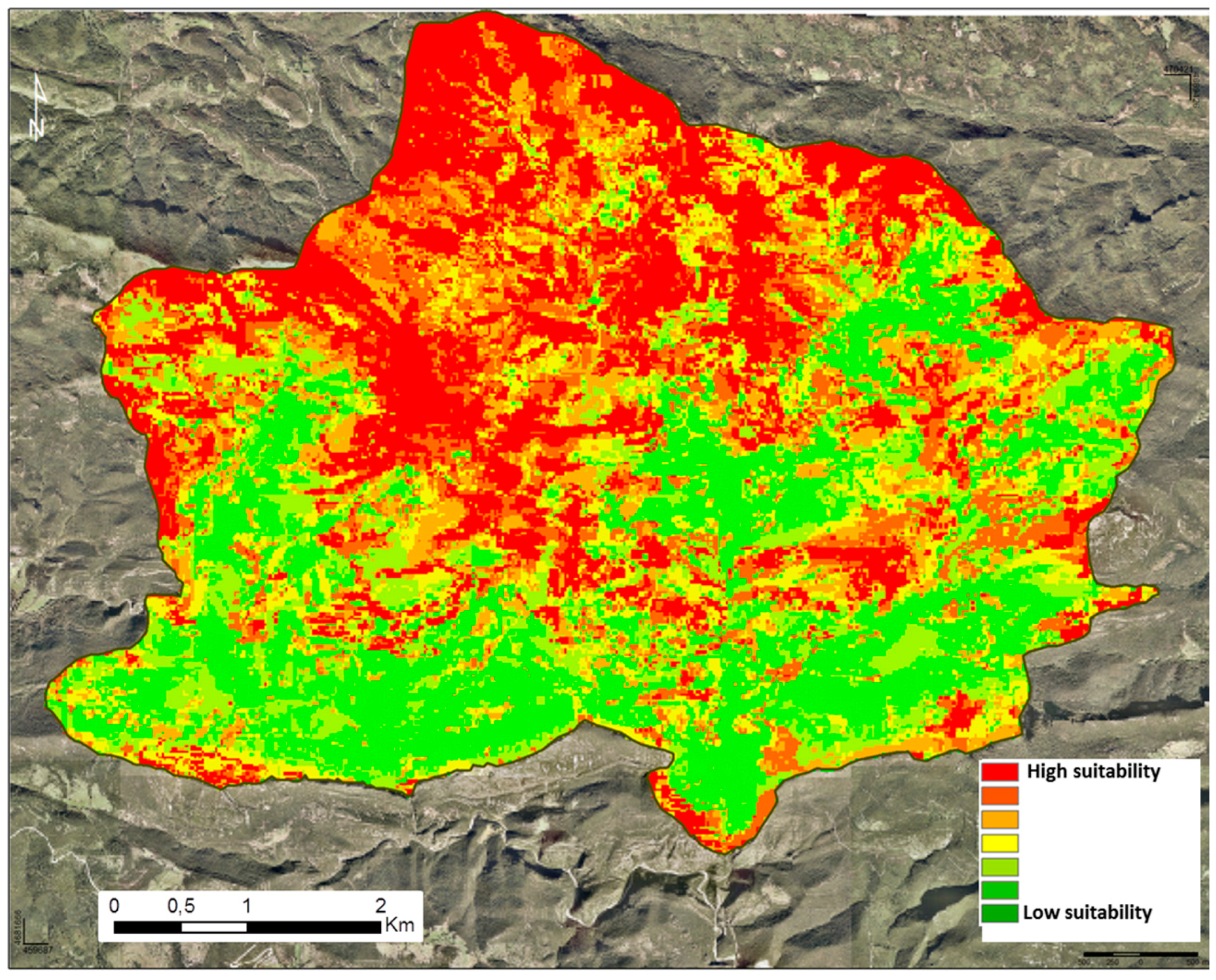
3.3. Suitability Map Results for the Recovery of Agrarian Land
4. Discussion
5. Conclusions
Acknowledgments
Author Contributions
Conflicts of Interest
References
- Llausàs, A.; Ribas, A.; Varga, D.; Vila, J. The evolution of agrarian practices and its effects on the structure of enclosure landscapes in the Alt Empordà (Catalonia, Spain), 1957–2001. Agric. Ecosyst. Environ. 2009, 129, 73–82. [Google Scholar] [CrossRef]
- Sevenant, M.; Antrop, M. The use of latent classes to identify individual differences in the importance of landscape dimensions for aesthetic preference. Land Use Policy 2010, 27, 827–842. [Google Scholar] [CrossRef]
- Mander, U.; Antrop, M. Multifunctional Landscapes. Volume III. Continuity and Change; Wit Press: Southampton, NY, USA, 2003; p. 304. ISBN 978-1-85312-935-3. [Google Scholar]
- Bielsa, I.; Pons, X.; Bunce, B. Agricultural Abandonment in the North Eastern Iberian Peninsula. The Use of Basic Landscape Metrics to Support Planning. J. Environ. Plan. Manag. 2005, 48, 85–102. [Google Scholar] [CrossRef]
- Jordan, N.; Warner, K.D. Enhancing the Multifunctionality of US Agriculture. BioScience 2010, 60, 60–66. [Google Scholar] [CrossRef]
- Boada, M. Boscos de Catalunya. In Història i Actualitat del món Forestal; Brau Edicions: Figueres, Catalonia, 2003; p. 188, (In Catalan). ISBN 84-95946-20-3. [Google Scholar]
- Cohen, M.; Varga, D.; Vila, J.; Barrassaud, E. A multi-scale and multi-disciplinary approach to monitor landscape dynamics: A case study in the Catalan pre-Pyrenees (Spain). Geogr. J. 2011, 177, 79–91. [Google Scholar] [CrossRef]
- McDonald, D.; Crabtree, J.R.; Wiesinger, G.; Dax, T.; Stamou, N.; Fleury, P.; Gutierrez Lazpita, J.; Gibon, A. Agricultural abandonment in mountain areas of Europe: Environmental consequences and policy response. J. Environ. Manag. 2000, 59, 47–69. [Google Scholar] [CrossRef]
- Taillefumier, F.; Piegay, H. Contemporary land use changes in prealpine Mediterranean mountains: A multivariate GIS-based approach applied to two municipalities in the Southern French Prealps. Catena 2002, 51, 267–296. [Google Scholar] [CrossRef]
- Nassauer, J. Culture and changing landscape structure. Landsc. Ecol. 1995, 10, 229–237. [Google Scholar] [CrossRef]
- Lasanta, T.; González-Hidalgo, J.; Vicente-Serrano, S.; Sferi, E. Using landscape ecology to evaluate an alternative management scenario in abandoned Mediterranean mountain areas. Landsc. Urban Plan. 2006, 78, 101–114. [Google Scholar] [CrossRef]
- Bignal, E.; McCracken, D. Low-intensity farming systems in the conservation of the countryside. J. Appl. Ecol. 1996, 33, 413–424. [Google Scholar] [CrossRef]
- Pujantell, J. Les Manifestacions del Canvi Global en àrees de Muntanya Mediterrània. Un cas d’estudi al Baix Montseny. Ph.D. Thesis, Institute of Environmental Science and Technology (ICTA), Universitat Autònoma de Barcelona (UAB), Bellaterra, Spain, 2012. (In Catalan). [Google Scholar]
- González, J.; Palahí, M.; Pukkala, T. Integrating fire risk considerations in forest management planning in Spain. A landscape level perspective. Landsc. Ecol. 2005, 20, 957–970. [Google Scholar] [CrossRef]
- Sluiter, R.; Jong, M. Spatial patterns of Mediterranean land abandonment and related land cover transitions. Landsc. Ecol. 2007, 22, 559–576. [Google Scholar] [CrossRef]
- Naveh, Z.; Lieberman, A. Landscape Ecology. Theory and Application; Springer: New York, NY, USA, 1994; p. 360. ISBN 978-1-4757-2331-1. [Google Scholar]
- Badia, A.; Saurí, D.; Cerdan, R.; Llurdés, J. Causality and management of forest fires in Mediterranean environments: An example from Catalonia. Environ. Hazards 2002, 4, 23–32. [Google Scholar] [CrossRef]
- Loehle, C. Applying landscape principles to fire hazard reduction. For. Ecol. Manag. 2004, 198, 261–267. [Google Scholar] [CrossRef]
- Fahrig, L. Effects of habitat fragmentation on biodiversity. Annu. Rev. Ecol. Evol. Syst. 2003, 34, 487–515. [Google Scholar] [CrossRef]
- Farina, A. The cultural landscape as a model for the integration of ecology and economics. BioScience 2000, 50, 313–320. [Google Scholar] [CrossRef]
- Antrop, M. Landscape change: Plan or chaos? Landsc. Urban Plan. 1998, 41, 155–161. [Google Scholar] [CrossRef]
- Conti, G.; Fagarazzi, L. Sustainable mountain development and the key-issue of abandonment of marginal rural areas. Planum 2004, 11, 1–19. [Google Scholar]
- Baldwin, D.; Weaver, K.; Schnekenburger, F.; Perera, A. Sensitivity of landscape pattern indices to input data characteristics on real landscapes: Implications for their use in natural disturbance. Landsc. Ecol. 2004, 19, 255–271. [Google Scholar] [CrossRef]
- Forman, R.; Godron, M. Landscape Ecology; Wiley and Sons: New York, NY, USA, 1986; p. 619. ISBN 978-0-471-87037-1. [Google Scholar]
- McGarigal, K.; Marks, B. FRAGSTATS: Spatial Pattern Analysis Program for Quantifying Landscape Structure; Department of Agriculture: Washington, DC, USA, 1995; p. 141.
- Farina, A. Principles and Methods in Landscape Ecology. Towards a Science of the Landscape; Springer: London, UK, 2006; p. 412. ISBN 13 978-1-4020-3329-2. [Google Scholar]
- Food and Agriculture Organization (FAO). The Development of European Forest Resources, 1950 to 2000: A Better Information Base; United Nations: Geneva, Switzerland, 2003; p. 108. [Google Scholar]
- Gustafson, E. Quantifying landscape spatial pattern: What is the state of the art? Ecosystems 1998, 1, 143–156. [Google Scholar] [CrossRef]
- Botequilha, A.; Miller, J.; Ahern, J.; MacGarigal, K. Measuring Landscapes. A Planner’s Handbook; Island Press: Washington, DC, USA, 2006; p. 272. ISBN 1-4020-3978-6. [Google Scholar]
- Craig, W.; Harris, T.; Weiner, D. Community Participation and GIS; Taylor & Francis: London, UK, 2002; p. 416, ISBN 13: 978-0415237529. [Google Scholar]
- Crossetto, M.; Crossetto, F.; Tarantola, S. Optimized resource allocation for GIS based model implementation. Photogramm. Eng. Remote Sens. 2002, 68, 225–232. [Google Scholar]
- Malczewski, J. GIS-based multicriteria decision analysis: A survey of the literature. Int. J. Geogr. Inf. Sci. 2006, 20, 703–726. [Google Scholar] [CrossRef]
- Eastman, J.R.; Jin, W.; Kyem, P.A.K.; Toledano, J. Raster procedure for Multi-Criteria/Multi-Objective Decisions. Photogramm. Eng. Remote Sens. 1995, 61, 539–547. [Google Scholar]
- Saaty, T. A scaling method for priorities in hierarchical structures. J. Math. Psychol. 1977, 15, 231–281. [Google Scholar] [CrossRef]
- Saaty, T. Decision-making with the AHP: Why is the principal eigenvector necessary? Eur. J. Oper. Res. 2003, 145, 85–91. [Google Scholar] [CrossRef]
- Modica, G.; Laudari, L.; Barreca, F.; Fichera, C.R. A GIS-MCDA Based Model for the Suitability Evaluation of Traditional Grape Varieties: The Case-Study of “Mantonico” Grape (Calabria, Italy). Int. J. Agric. Environ. Inf. Syst. 2014, 5, 1–16. [Google Scholar] [CrossRef]
- Anselin, A.; Meire, P.M.; Anselin, L. Multicriteria techniques in ecological evaluation: An example using the analytical hierarchy process. Biol. Conserv. 1989, 49, 215–229. [Google Scholar] [CrossRef]
- Marinoni, O. Implementation of the analytical hierarchy process with VBA in ArcGis. Comput. Geosci. 2004, 30, 637–646. [Google Scholar] [CrossRef]
- Palmer, J. Using spatial metrics to predict scenic perception in a changing landscape: Dennis, Massachussets. Landsc. Urban Plan. 2004, 69, 201–218. [Google Scholar] [CrossRef]
- Sherrouse, B.C.; Clement, J.M.; Semmens, D.J. A GIS application for assessing, mapping, and quantifying the social values of ecosystem services. Appl. Geogr. 2011, 31, 748–760. [Google Scholar] [CrossRef]
- Espunya, C.; Gallart, Q. Estudi de l’estat de Conservació del Patrimoni Monumental de l’Alta Garrotxa; Col·legi d’Arquitectes de Catalunya: Barcelona, Spain, 2004; p. 100. (In Catalan) [Google Scholar]
- Chuvieco, E.; Salas, J. Mapping the spatial distribution of forest fire danger using GIS. Int. J. Geogr. Inf. Syst. 1996, 10, 333–345. [Google Scholar] [CrossRef]
- Terra de Bosc. Pla de Prevenció d’incendis de l’Alta Garrotxa; Consorci de l’Alta Garrotxa: Barcelona, Spain, 2006. [Google Scholar]
- Ecological and Forestry Applications Research Center (CREAF). Map of Flammability Models, 2nd ed. (expanded). Available online: http://www.creaf.uab.cat/mmci/descarrega.htm (accessed on 31 July 2017).
- Climate Atlas of Catalonia. Available online: http://www.opengis.uab.cat/acdc/ (accessed on 25 October 2016).
- Regos, A.; Ninyerola, M.; Moré, G.; Pons, X. Linking land cover dynamics with driving forces in mountain landscape of the Northwestern Iberian Peninsula. Int. J. Appl. Earth Obs. Geoinf. 2015, 38, 1–14. [Google Scholar] [CrossRef]
- Otero, I.; Marull, J.; Tello, E.; Diana, G.L.; Pons, M.; Coll, F.; Boada, M. Land abandonment, landscape, and biodiversity: Questioning the restorative character of the forest transition in the Mediterranean. Ecol. Soc. 2015, 20, 7. [Google Scholar] [CrossRef]
- Peñuelas, J.; Sardans, J.; Filella, I.; Estiarte, M.; Llusià, J.; Ogaya, R.; Carnicer, J.; Bartrons, M.; Rivas-Ubach, A.; Grau, O.; et al. Impacts of Global Change on Mediterranean Forests and Their Services. Forests 2017, 8, 463. [Google Scholar] [CrossRef]
- Geri, F.; Amici, V.; Rocchini, D. Spatially-based accuracy assessment of forestation prediction in a complex Mediterranean landscape. Appl. Geogr. 2011, 31, 881–890. [Google Scholar] [CrossRef]
- Varga, D.; Vila, J. Ecología del paisaje y sistemas de información geográfica ante el cambio socioambiental en las áreas de montaña mediterránea. Una aproximación metodológica al caso de los valles d’Hortmoier y Sant Aniol (Alta Garrotxa. Girona). AREAS Revista Internacional de Ciencias Sociales 2005, 25, 59–72. [Google Scholar]
- Herrador, D.; Boada, M.; Varga, D.; Mendizábal, E. Tropical forest recovery and socio-economic change in El Salvador An opportunity for the introduction of new approaches to biodiversity protection. Appl. Geogr. 2011, 31, 259–268. [Google Scholar] [CrossRef]
- Loepfe, L.; Martinez-Vilalta, J.; Oliveres, J.; Piñol, J.; Lloret, F. Feedbacks between fuel reduction and landscape homogenisation determine fire regimes in three Mediterranean areas. For. Ecol. Manag. 2010, 259, 2366–2374. [Google Scholar] [CrossRef]
- Klein, D.; Sutherland, W. How effective are European agri-environment schemes in conserving and promoting biodiversity? J. Appl. Ecol. 2003, 40, 947–969. [Google Scholar] [CrossRef]


| Classes |
|---|
| Closed forest (>90%) |
| Dense forest (60–90%) |
| Open forest on pasture (10–60%) |
| Open forest on pan (10–60%) |
| Crops |
| Denuded |
| Building |
| Pasture |
| Track roads |
| Rivers |
| Indices | Description | Units |
|---|---|---|
| MPS | Average patch size for a landscape | Hectares |
| PD | Number of patches per 100 ha for a landscape | Number per 100 hectares |
| ED | Length of edge per hectare for a landscape | Meters per hectare |
| GYRATE | Equals the mean distance (m) between each cell in the patch and the patch centroid. It is a measure of patch extent; thus, it is effected by both patch size and patch compaction | Meters |
| PAFRAC | Degree of complexity of patches based on a perimeter to-area ratio | None |
| ENN | Equals the distance (m) to the nearest neighbouring patch of the same type, based on shortest edge-to-edge distance | Meters |
| COHESION | Measures the physical connectedness of the corresponding patch type | None |
| SHEI | It is expressed such that an even distribution of area among patch types results in maximum evenness. As such, evenness is the complement of dominance | None |
| Criteria | Conservation Scenario | Neutral Scenario | Management Scenario |
|---|---|---|---|
| Biodiversity | 45% | 20% | 4% |
| Lanscape configuration | 28% | 20% | 7% |
| Cultural Heritage | 16% | 20% | 16% |
| Fire risk | 7% | 20% | 28% |
| Management cost | 4% | 20% | 45% |
| Consistency Ratio (CR < 0.1) | 0.0237 | 0 | 0.0237 |
| Classes | ∆ ha. 2009–1957 | ∆ % 2009–1957 |
|---|---|---|
| Closed forest (>90%) | 2396.61 | 140.76 |
| Dense forest (60–90%) | −580.30 | −87 |
| Open forest on pasture (10–60%) | −493.93 | −62.68 |
| Open forest on pan (10–60%) | 2.45 | 1.59 |
| Crops | −149.05 | −96.38 |
| Denuded | −0.67 | −0.56 |
| Building | −1.37 | −55.75 |
| Pasture | −1112.04 | −76.87 |
| Track roads | −63.93 | −74.53 |
| Rivers | −0.02 | −0.06 |
| 1957 | 2009 | |||||||
|---|---|---|---|---|---|---|---|---|
| Closed Forest | Dense Forest | Open Forest on Pasture | Open Forest on Pan | Crops | Denuded | Pastures | Others | |
| Closed forest | 89.6 | 2.21 | 2.92 | 2.32 | 0 | 0 | 2.67 | 0.28 |
| Dense forest | 82.69 | 3.53 | 4.42 | 6.57 | 0 | 0 | 2.66 | 0.13 |
| Open forest on pasture | 79.42 | 6.81 | 5.64 | 0 | 0 | 0 | 7.82 | 0.31 |
| Open forest on pan | 68.37 | 0 | 0 | 24.6 | 0 | 7.03 | 0 | 0 |
| Crops | 57.05 | 0 | 16.23 | 0 | 3.5 | 0 | 23.22 | 0 |
| Pastures | 73.34 | 1.97 | 11.74 | 0 | 0 | 1.21 | 11.74 | 0 |
| Classes | ∆MPS | ∆PD | ∆ED | ∆GYRATE | ∆PAFRAC | ∆ENN | ∆COHESION |
|---|---|---|---|---|---|---|---|
| Closed forest (>90%) | 4084.83 | −3.6 | −57.72 | −40.53 | −0.09 | −19.13 | 0.41 |
| Dense forest (60–90%) | 1.8 | −4.81 | −79.05 | 4.49 | 0.01 | 921.52 | −0.12 |
| Open forest on pasture (10–60%) | −3.61 | 2.99 | −59.24 | −44.21 | −0.02 | 58.83 | −2.23 |
| Open forest on pan (10–60%) | −1.31 | 1.08 | −11.68 | −57.25 | 0.08 | −19.24 | −5.47 |
| Crops | −0.26 | −2.41 | −9.81 | −9.76 | 0.14 | 466.84 | −0.22 |
| Pasture | −4.28 | 1.1 | −54.01 | −38.85 | 0.12 | 80.29 | −1.58 |
© 2018 by the authors. Licensee MDPI, Basel, Switzerland. This article is an open access article distributed under the terms and conditions of the Creative Commons Attribution (CC BY) license (http://creativecommons.org/licenses/by/4.0/).
Share and Cite
Varga, D.; Vila Subirós, J.; Barriocanal, C.; Pujantell, J. Landscape Transformation under Global Environmental Change in Mediterranean Mountains: Agrarian Lands as a Guarantee for Maintaining Their Multifunctionality. Forests 2018, 9, 27. https://doi.org/10.3390/f9010027
Varga D, Vila Subirós J, Barriocanal C, Pujantell J. Landscape Transformation under Global Environmental Change in Mediterranean Mountains: Agrarian Lands as a Guarantee for Maintaining Their Multifunctionality. Forests. 2018; 9(1):27. https://doi.org/10.3390/f9010027
Chicago/Turabian StyleVarga, Diego, Josep Vila Subirós, Carles Barriocanal, and Josep Pujantell. 2018. "Landscape Transformation under Global Environmental Change in Mediterranean Mountains: Agrarian Lands as a Guarantee for Maintaining Their Multifunctionality" Forests 9, no. 1: 27. https://doi.org/10.3390/f9010027
APA StyleVarga, D., Vila Subirós, J., Barriocanal, C., & Pujantell, J. (2018). Landscape Transformation under Global Environmental Change in Mediterranean Mountains: Agrarian Lands as a Guarantee for Maintaining Their Multifunctionality. Forests, 9(1), 27. https://doi.org/10.3390/f9010027