The Impact of Assumed Uncertainty on Long-Term Decisions in Forest Spatial Harvest Scheduling as a Part of Sustainable Development


1
Department of Forest Management, Faculty of Forestry and Wood Sciences, Czech University of Life Sciences Prague, Kamýcká 129, Praha–Suchdol 16500, Czech Republic
2
Department of Systems Engineering, Faculty of Economics and Management, Czech University of Life Sciences Prague, Kamýcká 129, Praha–Suchdol 16500, Czech Republic
*
Author to whom correspondence should be addressed.
Forests 2017, 8(9), 335; https://doi.org/10.3390/f8090335
Submission received: 9 August 2017
/
Revised: 31 August 2017
/
Accepted: 7 September 2017
/
Published: 8 September 2017
(This article belongs to the Special Issue Forest Sustainable Management)
Abstract
:The paper shows how the aspects of uncertainty in spatial harvest scheduling can be embedded into a harvest optimization model. We introduce an approach based on robust optimization that secures better scheduling schematics of the decision maker while eliminating a significant portion of uncertainty in the decisions. The robust programming approach presented in this paper was applied in a real management area of Central Europe. The basic harvest scheduling model with harvest-flow constraints was created. The uncertainty that is assessed here is due to forest inventory errors and growth prediction errors of stand volume. The modelled results were compared with randomly simulated errors of stand volume. The effects of different levels of robustness and uncertainty on harvest-flow were analyzed. The analysis confirmed that using the robust approach for harvest decisions always ensures significantly better solutions in terms of the harvested volume than the worst-case scenarios created under the same constraints. The construction of a mathematical model as well as the methodology of simulations are described in detail. The observed results confirmed obvious advantages of robust optimization. However, many problems with its application in forest management must still be solved. This study helps to address the need to develop and explore methods for decision-making under different kinds of uncertainty in forest management.
1. Introduction
According to the Food and Agriculture Organization [1], one form of sustainable indicator is the area of forests under sustainable forest management. Sustainable development is a necessary part of sustainable forest management and its purpose is to eradicate poverty, to significantly minimize deforestation, and to minimize degradation of natural resources (forests) and the loss of biodiversity of the forests. Forest management should reduce possible fluctuations in the harvested amount of wood that could cause excessive deforestation and thereby reduce all ecosystem services. However, there are a lot of uncertainties in forestry-timber sector which can significantly impair the functioning of the entire supply chain and thus decrease the efficiency of use [2]. Uncertainty means lack of the information about the current or future state of the forest. The quality of forest management and planning has an important direct impact on the performance of the supply chain [3].
Although forestry and timber supply chains have been improved during the last decade, the challenge of integrating different planning problems still remains. For example, long-term forest management requires assumptions about future conditions which have various degrees of uncertainty. Wrong decisions in forest management can have effects that span over long periods [4]. Although deterministic models can provide relatively good solutions, they do not take into account the information about variability of the incomes caused by these sources of uncertainty.
One way to incorporate uncertainty into the planning process is post-optimal or sensitivity analysis, while another approach used in forestry is based on scenario analyses or simulations. The uncertainty in the modelling process [5] can be explicitly considered by the means of the mathematical programming methods which have been used to solve harvest scheduling problems since the 1970s (e.g., [6,7]). Any harvest scheduling model should also include harvest-flow constraints which are essential parts of these models because coordinating the harvest-flow is a vital concern of many forest and timber companies [8]. There are many different types of harvest-flow constraints presented in many different papers (see, for example, [9,10,11]).
Parameter uncertainty in mathematical programming has been treated in many ways since Dantzig’s pioneering work [12] wherein the sensitivity analysis of the mathematical programs is introduced. The sensitivity analysis is a tool that allows ex-post examination of possible perturbations in the input data. Ben-Tal and Nemirovski [13] point out, however, that the sensitivity analysis does not say how to improve the solution stability when necessary and instead, they focus on robust optimization methodology (RO) which is a possible approach to deal with the uncertainty. Also, RO is deterministic and set-based rather than stochastic programming [14]. An overall comparison of robust optimization, stochastic (linear) programming, and sensitivity analysis is brought by Mulvey, Vanderbei, and Zenios [15] who also provide the comparison of all approaches on the real case study which is built on earlier robust formulation developed by Malcolm and Zenios [16]. An extensive work on the matter of robustness was developed by Soyster [17]. Compared to the current trends in robust optimization, it was quite over-conservative in terms of uncertainty. Since Soyster’s work, a considerable number of improvements were made in this area and RO has become a focus of many researchers, as it happens to be somehow attractive for its not-so-stochastic nature. Not only is it applicable to linear programs, but it was generalized for integer programming [18] or even semidefinite programming (SDP). Despite semidefinite programming being a rather new field of optimization, it has come to interest of researchers dealing with robustness. El-Ghaoui, Oustry, and Lebret [19] prove and show how to obtain approximate robust solutions via SDP.
Several scientific papers dealing with RO have already been published on this matter. Palma and Nelson [5] applied the RO approach in a typical harvest scheduling problem where the uncertainty is considered in the volume and demand of products over the entire planning horizon. They took advantage of the approach by Bertsimas and Sim [19] with slight changes proposed in the paper [5]. Later on, Palma described the usefulness of RO within the harvest decisions from several different points of view [20]. Another paper by Palma and Nelson [21] is dedicated to the RO of road-building and harvest-scheduling decisions from timber estimate errors. Another paper dealing with road building and uncertainty was elaborated by Murphy and Stander [22]. From recent papers looking at the robust optimization in the field of forestry, we can mention two papers dedicated to sawmill planning [23,24] and sawmill production scheduling [25]. One can notice that the RO approach appears in the forestry science quite rarely and only in recent years.
The main goal of the paper is to analyze possible effects of assumed uncertainties in forestry inventory data and growth model predictions on the harvesting balance in the long-term perspective and to present one possible method of incorporating the uncertainties directly into the harvest scheduling model. The second goal of the paper is to test a new way of including robustness into the harvest scheduling model.
2. Materials and Methods
2.1. Study Area
The models were applied to a 513.9 ha forest management unit (FMU) located in the central part of the Czech Republic with mean altitude of 510 m above sea level. The mean rotation period is 110 years and the regeneration period is 30 years. The stand volume data for this FMU were obtained from the forest inventory documents in 2013. To simplify the scenarios, species composition of the forest stands was limited to a single species, Norway spruce (Picea abies (L.) Karst), which covers 87% of the FMU. We used the current mean site index of the studied FMU equal to 28. One hundred and sixty-three (163) stands with a total area of 350 ha were available to be harvested in the initial 50 years. Each forest stand was divided into the harvest units (strips) following the rules of the clear-cut system (i.e., the limited area and the width of strips). The total number of harvest units was 361, with an average area of 0.96 ha. A planning horizon of five periods (each 10 years long) was used for the analysis.
2.2. Model Formulation
In this section, we introduce two harvest scheduling models. Firstly, the deterministic model (DET) of harvesting will be specified and the robust model (ROB) and its development from the first model (DET) will be described. The DET model represents a deterministic description of the harvest scheduling situation where no uncertainty is assumed. The ROB model describes the analogous situation but with aspects of uncertainty also included. Both models are described further in detail.
The DET maximizes the volume of the harvest units over a certain number of harvest periods while the harvest balance across the planning horizon as well as the spatial restrictions between the cutting units are preserved. This model generally falls into the category of Unit restriction models of spatial harvest scheduling (URM), which specifically proposes harvesting not only in the time but also in the space. The DET model is a discrete programming model and consists of a set of decision 0–1 variables , four sets of constraints and one objective function. The model is generally applied to cutting units over periods, and the indices of decision variables are and .
The optimization goal is given as the maximization of the harvested volume under the constraints that harvesting fluency, unit adjacency, and other logical conditions are satisfied. For modelling purposes, we assumed 5% growth from period to period. Let us denote the DET model as:
subject to
The objective function (1) maximizes the harvested volume of each unit in every period over the set of all units and the set of all periods . where expresses the stand volume. The first set of constraints (2) ensures that each unit is harvested at most once during the planning horizon, the second set of constraints (3) ensures the fluent harvest flow with the maximum deviation such that and the third set of constraints (4) describes the spatial restrictions of the problem while the set includes all units adjacent to the unit . The last set of constraints (5) merely shows what values the decision variable can attain. The value of means the unit is not harvested in period , while shows the opposite. Let us denote the feasibility subset (2, 4, and 5) of DET as (defined later).
The solution of the DET model is based on the assumption that all exact parameter values of its components are known. Specifically, it is considered that the estimated volume of all harvest units is not going to change in any way over the planning horizon of periods. In practice, this is hardly a certainty with respect to all thinkable influences of environmental changes or human-caused actions.
It is possible to overcome these unexpected deviations by building a robust optimization model. A robust alternative to the standard deterministic optimization model is called a robust counterpart (ROB). In the following section, the modified approach of Palma and Nelson [5] (originally based on [26]) that accounts also for the robustness of left-hand side coefficients will be briefly summarized.
Let us have a general constraint of an optimization model given as . Let us assume that the coefficients belong to a symmetric interval , where is the expected symmetric deviation from the original deterministic value of the coefficient . To acquire the ROB model, one must perform several steps to transform the original model into its robust counterpart. The deviations shown in this paragraph refer to the changes in the left-hand side coefficients in an arbitrary constraint of an optimization problem given as:
subject to:
The robust counterpart of (6, 7) model is then defined as:
subject to:
There are several new variables and parameters in (8, 9) that need to be explained. Auxiliary variables and are products of the ROB model inference from the DET and have no significantly important real interpretation for our purposes. is an important parameter that controls the uncertainty for each constraint. The value of (protection level) represents how many left-hand side coefficients of that constraint we assume have deviations from their original values by . The set of indices is the set of uncertain coefficients that are considered for each constraint. We refer the reader to Bertsimas and Sim [26] for the detailed proof of creating (8, 9) from (6, 7).
Going back to our DET model, one can realize that imposing the uncertainty on any left-hand side coefficients in constraints (2–5) would be sensible only in the case of constraints (3). In the remaining constraints (2, 4, and 5), no such coefficients are explicitly included. In the case of (3), it could be assumed to impose the uncertainty on parameter or parameter(s) The parameter alone is given by the harvest-flow standards where no deviations can be logically assumed. The group of parameters is more of our interest since the volume of individual stands is a quantity that can be hardly measured with absolute precision. Thus, we will concentrate on assuming deflections in the parameters.
The s in the DET model are found in constraints (3) that express the ratio between the total volumes harvested in two consequent periods. One must notice that the very same parameters also appear in the objective function of the DET model. We can assume that the uncertainty of s must be then considered in both constraints (3) and objective function (1). We will apply the transformation from DET model (6, 7) to ROB model (8, 9) as described above. However, the given form of ROB (8, 9) assumes uncertainties only in the left-hand sided coefficients of the model constraints. In our case, the uncertainty is needed in the constraints and in the objective function. One can overcome this issue by transforming the objective function into a constraint in the following way:
Is equivalent to (11) with (12)
subject to
with as an auxiliary function. Now in (12) the objective function coefficients are on the left-hand side and hence, it is possible to treat them in terms of building a robust counterpart.
However, the number of expected deviations controlled by parameter is known. To solve it, let us assume that some of the s will deviate in the objective function (or now in constraint (12)) by at most . By setting to a specific value we state that this is the maximum possible number of coefficients that will possibly deviate from their expected values. However, the coefficients are not specified. Practically, it means that the number of the coefficients, which will change in every period , is unknown. This is a problem in relation to the set of constraints (3) wherein the same s are also included. To deal with this situation we have to split the objective function into a sum of functions with each representing one period. That leads to the following equivalent re-definition of (11) and (12) into:
subject to
This allows us to treat the uncertainty in the individual periods separately. It is now possible to design the final ROB model:
subject to
This was an expected obstacle since the problem is NP-hard (non-deterministic polynomial-time hard) on its own (due to the presence of integral variables). The time limit for solving had to be set to 1200 s. The instances of the described models were computed on a personal computer with Intel® Core ™ processor (Intel, Santa Clara, CA, USA) with 3.40 GHz and 16.0 GB random-access memory, which represents common computer equipment available today. The Gurobi® 6. 5 (Gurobi, Houston, TX, USA) [27] optimization solver was used. The branching solving algorithm allows for lower and upper bounds to be found on the optimal solution. The optimal solution might not be found in a reasonable time but the lower and upper bounds might be. This approach can sometimes provide a sufficiently tight estimate of the result. Once the lower and upper bounds on the optimal solution are available the software is able to calculate the feasible solution whose objective is within % of the optimum value . The difference between and is called a gap.
2.3. Simulation Experiments
The deterministic and robust solutions were tested by simulating the uncertain coefficients of the model within the uncertainty sets as described above. The slightly changed approach proposed by [5] was used for the simulation. That is, we analyzed the optimal solutions from the deterministic and robust models using randomly selected harvest units whose stand volumes were reduced by deviations defined above (). The number of the randomly selected harvest units was equal to the protection levels () for each individual planning period. We performed 1000 simulations of the volume coefficients for all optimal solutions. The same number of simulations was performed in the similar experiments by Palma [5]. In our case, it occurred that the higher number of simulations is not necessary for the refinement of the results. A convergent behavior was observed in the variance of the solutions above 1000 simulations, and thus we consider this number sufficient. The resulting objective function, change in the periodic harvested amount, and the occurrence of infeasibility were examined.
3. Results
Different harvest flow percentages (10% to 100% in scale of 10%) were analyzed in this paper for five planning periods. The uncertain parameters were used for the simulation experiments and the ROB model. We assumed the deviation equal to 15% for the first planning period (PP), 20% for the second PP, 25% for the third PP, 30% for fourth PP, and 35% for the fifth PP. The assumptions of the deviations are based on the theoretical expectation of the inventory errors in the first PP which increase in each period by the approximated prediction errors. The protection levels were set to 10% to 60% for the first PP. It is assumed that 10% to 60% of the harvest units can have negative deviations from the original value in the first PP. We assumed that the confidence in the predicted number of deviations decreases with every subsequent PP; in other words, the protection level increases by 10% in each PP.
Figure 1 presents the relation between the protection level and the harvested volume estimated by simulation experiments for each period. The optimal solution from the DET model was used for the simulation experiments and is presented by the black squares in the figure. The harvest flow constraints were excluded from this DET model. It is obvious that as the planning period and the expected uncertainty of growth increase, the difference between the expected harvested volume (DET model value) and the simulated worst alternative of the harvested volume also increase. Contrary to other works (e.g., [5]), simulations were always worse (100% of cases) than the solution obtained by the DET model, or always better (100% of cases) than the solution obtained by the ROB model.
The results for the DET model that include the harvest flow constraints for 50% protection level in the first PP are presented in Table 1. Only one initial size of protection level was selected for a clear presentation of the results. It is obvious that as the harvest flow percentage increases the total harvested volume also increases. However, the difference in the total harvested volume (objective function of the DET model) is more than 4% between 10% and 100% harvest flow. The harvested volume increases with the period index because of the growth of the forests. The harvest flow constraints do not affect the total harvested volume significantly but they are necessary for the harvest flow preservation. The exclusion of the harvest flow constraints from the model or too high values of the harvest flow percentage can have a significant negative impact on the ecosystem in the future without any significant economic effect.
The results of the simulation using the DET model show (Table 2) that as the harvest flow percentage decreases the total harvested volume increases. The simulated total harvested value from the DET model without the harvest flow is also worse than the DET model´s results without the harvest flow constraints. This means that the harvest flow constraints do not affect the total harvested volume under uncertainty. However, the highest total harvested volume is obtained without the harvest flow constraints by simulations as well as the DET model.
If the results from the DET model and simulation experiments are compared, one can see that no value from the simulations is better than the values obtained using the DET model. Moreover, no value of the periodic harvested volume obtained from the DET model is within the range of simulations given by standard deviations. The worst alternatives of the harvested volumes will therefore always be lower than expected according to the harvest scheduling plan.
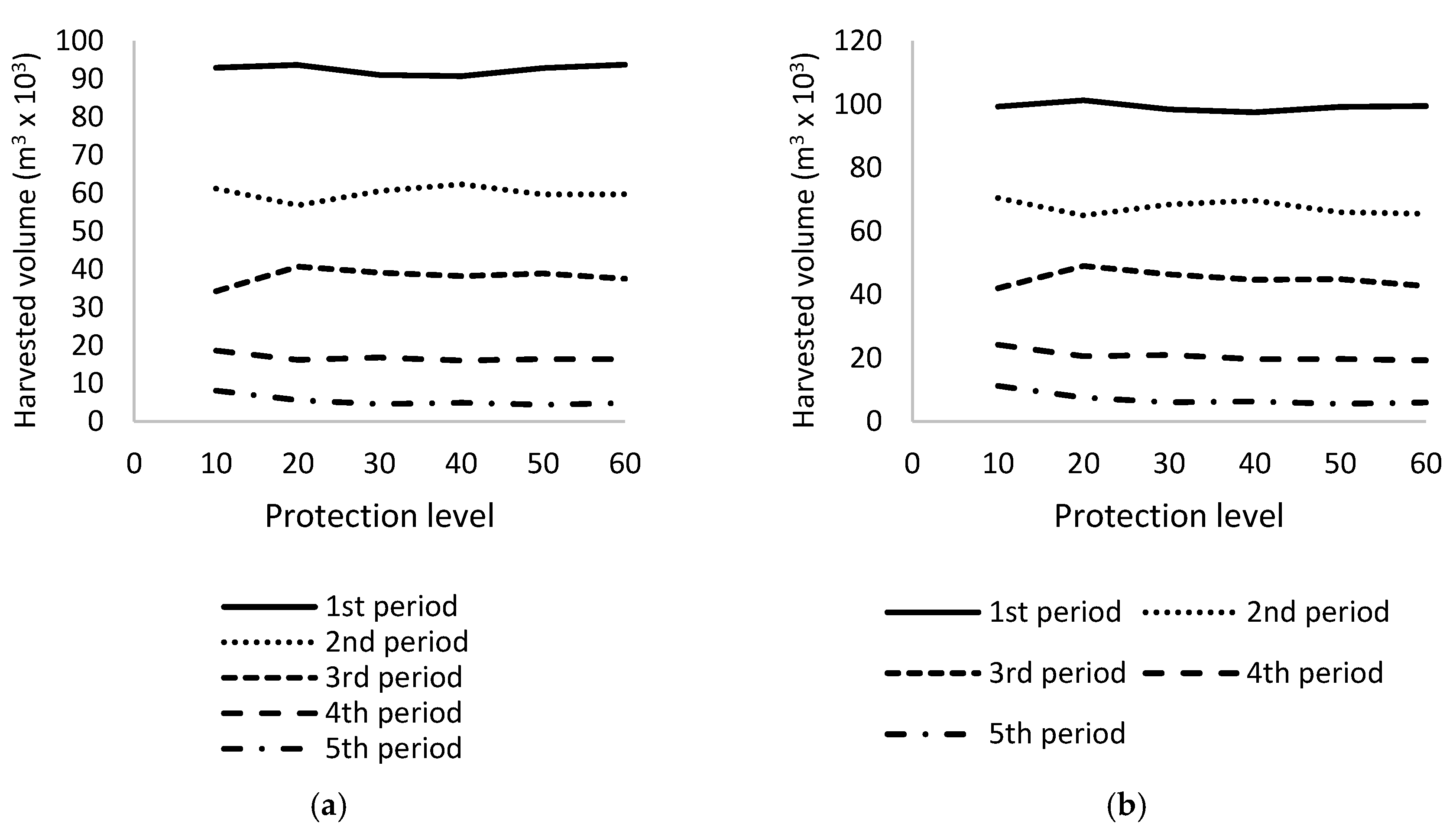
Unlike the DET model results (without the harvest flow constraints), the relations between the protection level and the harvested volume obtained from the ROB model and simulation experiments for each period are more similar (Figure 2). There is therefore no big difference between the expected value (ROB model) and the worst possible real alternative (simulated values). Moreover, all of the simulated worst possible alternatives are better than expected by the ROB model, which can be understood as a success rate of simulations surpassing the ROB model results. On the other hand, the success rate of simulations over the DET model was 0.
At the beginning of the planning horizon (first PP), the harvested volume increases with the increasing protection level. However, in the middle and at the end of the planning horizon (third to fifth period), the harvested volume decreases as the protection level increases. It is necessary to emphasize that these relations are only valid for the models and simulations that do not contain the harvest flow constraints.
The results of the computations for the chosen instances are shown in Table 3. The table shows the influence of the harvest flow percentage with the combination of the protection level on the computation time measured in a gap tolerance. The scenarios with 10% up to 100% harvest flow were assumed with the initial protection level varying from 10% up to 60%. Note that it is not possible to inspect protection levels above 60% because we consider the protection level in the experiment methodology to raise by 10% in each period. Starting with 60% in the first period would result in 100% protection in the fifth period, which is the logical protection limit.
When both the harvest flow and the protection level were set to smaller values the optimal solution was found with zero objective, which means that no harvesting should be performed at all. This is caused by too strict requirements on the model in terms of protection and harvest flow and no solution where the units could be harvested exists. In general, the lower the harvest flow is the stricter the requirements are laid on the model and thus, the solution is not achievable at all or is achievable in a time that exceeds the practical usage of this approach.
One might argue that the use of the presented ROB models is impractical when it is not possible to achieve a low harvest flow. However, when the final harvest flow percentages are calculated for models and simulations results, one can see that the real (achieved) harvest flow is much lower than the expected one by the models (Table 4). The resulted harvest flows are presented just for the 50% protection level, as the situation is similar in other protection level alternatives as well. The positive value of percentages signifies the increase of the harvested amount between two consecutive periods, the negative value of percentages signifies the decrease of the harvested amount between two consecutive periods. Although the achieved harvest flow percentages are better than those expected by the ROB model even in the case of the simulations, the harvest flow during the planning horizon is not ensured.
The results of the ROB model including the harvest flow constraints for 50% protection level in the first PP are presented in Table 5. Only one initial size of the protection level was selected to ensure the clarity of the result presentation. The alternatives with the harvest flow percentage lower than 50% in which no solution was obtained are not presented for the same reason. It is obvious that the increase of the harvest flow percentage results in the higher total harvested volume similar to DET model results (Table 1). The simulated values of the harvested amount in each period are higher than the expected amount obtained by the ROB model (Table 6). This difference is obvious especially in the first periods.
The total harvested amount of the ROB model during the whole planning horizon is much lower than the total harvested amount in the case of the DET model. However, the simulated values of the ROB model (Table 6) are higher than the simulated values of the DET model (Table 2). This means that the realized harvest situation will always be better than the planned harvest, and that is the main important advantage of the RO.
4. Discussion
The sustainable use of natural resources is not only about the balanced harvesting or economic profit. Sustainable management aimed at sustainable development must include all services provided by the natural resources. However, the economic prosperity significantly contributes to the social welfare. The prosperous company is then willing to reduce its demands on the fulfilment of production. Moreover, the unexpected fluctuations in harvesting can cause excessive ecosystem loading by trying to ensure stable financial incomes for the company and employees. Balanced harvesting is a necessary part of sustainable development. Mathematical programming methods have been widely used for harvest scheduling since the 1970s, and harvest flow constraints have been an important part of all developed models [28]. The great importance of the harvest flow constraints to the optimal solution is evident from the presented results. However, there are a lot of sources of uncertainties and risks in forest management which can significantly disturb the flow of harvesting. Some of them are difficult to predict, such as climate conditions or natural disturbances. Those sources of uncertainty that can be at least approximately predicted should therefore be a part of harvest scheduling processes.
The RO is one of the approaches used to incorporate the uncertainties into the harvest scheduling. The RO is under the focus of many researchers because of its not-so-stochastic nature. Palma and Nelson [5] based the robustness (a) on the minimal demand of harvested amount condition, or (b) on the protection against infeasibility for volume-fluctuation constraints. However, they applied the model to a linear programming model in which spatial details cannot be included. Models integrating spatial aspects are needed in the long-term planning process because of certification requirements, aesthetic concerns, fragmentation issues, etc. [29]. In another work, Palma and Nelson [21] applied robust programming to a binary programming problem, however, they did not test the effect of robustness on the harvest flow. This paper concentrates more on testing the uncertainty in the harvest flow constraints in spatial harvest scheduling models. Moreover, the goal of the paper was to test different harvest flow percentages as opposed to the mentioned authors who were more focused on testing different types of protection levels. However, if the forest sector plays a great role in the bioeconomy [30], quality and reliable harvest scheduling that includes spatial details as well as harvest flow conditions is needed.
The value of the protection level () is a very important parameter of RO because it represents how many left-hand side coefficients of that constraint we assume have deviations from their original values. In other words, this value shows how many variables (harvest units) can have negative deviations from their deterministic values (i.e., in a sense it shows the size of the user's confidence in the predicted deviations). The robust harvest scheduling model presented in this paper includes robustness based on harvest-flow conditions for each planning period. The advantage of the RO is that the optimal solution will be better and a higher success rate than the worst possible real situation. When the robustness is laid on an objective function, it is ensured that the total harvested amount will be higher than the value of the objective function of a RO model. However, it cannot be ensured that the partial harvested amounts in individual periods will actually be better than what a RO model gives. The results of the simulations based on the ROB model presented in this study are always better than the ROB model results even in the partial periods.
The first discovered complication of the presented approach is the computational complexity, which seems to be an obstacle for its practical use. The computational experience reveals the need to test various heuristic methods for pre-solving the robust models with harvest flow constraints, as in the case of complex spatial harvest scheduling problems (see, for example, [31]). Palma and Nelson [5] also draw attention to the problem of the size of robust programming models, but point out that the models are still linear, which is their greatest advantage. General linear programming problem has n variables and m + n constraints (n is the number of non-negativity constraints). A general robust model has n + m + m × n variables and 3m + n + 2m × p, where p is the number of variables considered where uncertainty occurs. In addition, in the presented model, we are still transferring the objective function into the constraints, so the increase will be even higher.
Additionally, there is an obvious correlation between the level of protection, harvest flow, and computational time altogether. In the case of the harvest flow greater than or equal to 50%, it is evident that with growing protection levels the gap tolerance approaches zero. We assume that the decrease in gap tolerances originates in the general behavior of the gamma-robustness models. The presented approach of robust optimization generally tends to choose those basic variables (i.e., those harvest units that are going to be harvested) to incorporate into the optimal solution for which the uncertainty is assumed. If there is only a small percent of the units with the considered uncertainty, it is assumed that these units will be preferably chosen for harvesting, but then it is necessary to choose and accompany them with other units where the uncertainty is not considered. In the case of a higher number of uncertain units, the model assumes that those will be incorporated into the solution (if feasible) and then it spends less time searching for other deterministic units to incorporate into the solution. This tendency was observed by Hlavatý and Brožová [32] who performed calculation experiments with the same approach to model robustness on a simpler linear programming case.
The results could be different when a different initial age structure is used. In this paper, the real age structure of the forest was used, so the results could not be generalized for any kind of forest structure. Testing of age structure influence on the RO results was not yet done and could be the key point for ongoing research.
The RO provides a robust optimal solution, which in reality will always be better than the actual schedule. Contrary to other works (e.g., [5]), simulations were always better (100% of cases) than the solution obtained by the ROB model. Unlike the deterministic model, a larger amount of timber will be harvested than the optimal solution suggests, because this solution is calculated using the worst-case (negative deviations) alternatives of stand volumes. The harvested volume reduction is referred to as a price of robustness. However, the extreme positive deviations can also significantly affect the harvest flow. Unfortunately, this characteristic could not be incorporated into the harvest scheduling process by the presented approach because of the nature of RO. A potential approach is called multi-band robust programming, as proposed by D’Andreagiovanni and Raymond [33].
There is an obvious advantage in the use of RO due to its not-so-stochastic nature. However, stochastic programming has already been used for harvest scheduling models under uncertainty as well (see, for example, [34,35]). As was shown above, many problems facing the full applicability of RO for forest management must still be solved.
5. Conclusions
The uncertainty caused by human errors and natural impacts majorly affects forest management and harvest scheduling, especially from a long-term point of view. Despite this mentioned fact, the presented impacts of uncertainty were marginally included in practical forest management. It is obvious that to ensure sustainability, harvest scheduling approaches must include uncertainty sources as much as possible to avoid extreme fluctuations of harvesting during the planning horizon. The fluctuations in harvesting can negatively affect not only forest-timber supply chains but also forest ecosystems. Classical methods of harvest scheduling are not able to include uncertainty, while the presented robust optimization approach can be considered as a possible manner in which to make forest planning more realistic. Although many sources of uncertainty are not included in the presented analysis (climate change, timber market prices, etc.) for methodological reasons, it is obvious that it is necessary to further develop and explore methods that can help to make a right decision in the rapidly changing world. The uncertainty should be reduced as much as possible by also minimizing human errors or improving prediction models.
Acknowledgments
This research was supported by the project of the National Agency for Agriculture Research (No. QJ1320230).
Author Contributions
Jan Kašpar established the idea and directed the development of the mathematical formulation of the harvest scheduling model. Robert Hlavatý was responsible for the mathematical formulation. Karel Kuželka determined the uncertainty for the purposes of this paper. Róbert Marušák was the supervisor for this work.
Conflicts of Interest
The authors declare no conflict of interest. The founding sponsors had no role in the design of the study; in the collection, analyses, or interpretation of data; in the writing of the manuscript, and in the decision to publish the results.
References
- FAO. Indicators of Sustainable Development: Guidelines and Methodologies, 3rd ed.; United Nations Publications: New York, NY, USA, 2007; ISBN 978-92-1-104577-2. [Google Scholar]
- Gertner, G.; Köhl, M. An assessment of some nonsampling errors in a national survey using an error budget. For. Sci. 1992, 38, 525–538. [Google Scholar]
- D’Amours, S.; Rönnqvist, M.; Weintraub, A. Using operational research for supply chain planning in the forest products industry. INFOR 2008, 46, 265–281. [Google Scholar] [CrossRef]
- Pasalodos-Tato, M.; Mäkinen, A.; Garcia-Gonyalo, J.; Borges, J.G.; Lämås, T.; Eriksson, L.O. Review. Assessing uncertainty and risk in forest planning and decision support systems: Review of classical methods and introduction of innovative approaches. For. Syst. 2013, 22, 282–303. [Google Scholar] [CrossRef]
- Palma, C.D.; Nelson, J.D. A robust optimization approach protected harvest scheduling decisions against uncertainty. Can. J. For. Res. 2009, 39, 342–355. [Google Scholar] [CrossRef]
- Johnson, K.; Scheurman, H. Techniques for prescribing optimal timber harvest and investment under different objectives—Discussion and synthesis. Forest Sci. 1977, 23, 1–31. [Google Scholar]
- Field, R. C.; Dress, P. E.; Fortson, J. C. Complementary linear and goal programming procedures for timber harvest scheduling. Forest Sci. 1980, 26, 121–133. [Google Scholar]
- Carlsson, D.; Rönnqvist, N. Supply chain management in forestry—case studies at Södra Cell AB. Eur. J. Oper. Res. 2005, 163, 589–616. [Google Scholar] [CrossRef]
- McDill, M.E.; Rebain, S.A.; Braze, J. Harvest scheduling with area-based adjacency constraints. For. Sci. 2002, 48, 631–642. [Google Scholar]
- Gunn, E.A.; Richards, E.W. Solving the adjacency problem with stand-centered constraints. Can. J. For. Res. 2005, 65, 832–842. [Google Scholar] [CrossRef]
- Yoshimoto, A.; Brodie, J.D. Short- and long-term impacts of spatial restriction on harvest scheduling with reference to riparian zone planning. Can. J. For. Res. 1994, 24, 1617–1628. [Google Scholar] [CrossRef]
- Dantzig, G.B. Linear programming under uncertainty. Manag. Sci. 1955, 1, 197–206. [Google Scholar] [CrossRef]
- Ben-Tal, A.; Nemirovski, A. Robust solutions of linear programming problems contaminated with uncertain data. Math Progr. 2000, 88, 411–424. [Google Scholar] [CrossRef]
- Bertsimas, D.; Brown, D. B.; Caramanis, C. Theory and applications of robust optimization. SIAM Rev. 2011, 53, 464–501. [Google Scholar] [CrossRef]
- Mulvey, J.M.; Vanderbei, R.J.; Zenios, S.A. Robust optimization of large-scale systems. Oper. Res. 1995, 43, 264–281. [Google Scholar] [CrossRef]
- Malcolm, S.; Zenios, S.A. Robust optimization for power capacity expansion planning. J. Oper. Res. Soc. 1994, 45, 1040–1049. [Google Scholar] [CrossRef]
- Soyster, A.L. Convex programming with set-inclusive constraints and applications to inexact linear programming. Oper. Res. 1973, 21, 1154–1157. [Google Scholar] [CrossRef]
- Bertsimas, D.; Sim, M. Robust discrete optimization and network flows. Math Progr. 2003, 98, 49–71. [Google Scholar] [CrossRef]
- Palma, C.D. Robust Optimization for Forest Resources Decision-Making under Uncertainty. Ph.D. Thesis, The University of British Columbia, Vancouver, BC, Canada, 2010. [Google Scholar]
- El-Ghaoui, L.; Oustry, F.; Lebret, H. Robust solutions to uncertain semidefinite programs. SIAM J. Optim. 1998, 9, 33–52. [Google Scholar] [CrossRef]
- Palma, C.D.; Nelson, J.D. A robust model for protecting road-building and harvest-scheduling decisions from timber estimate errors. Forest Sci. 2014, 60, 137–148. [Google Scholar] [CrossRef]
- Murphy, G.; Stander, H.C. Robust optimisation of forest transportation networks: A case study. South Hemisph. For. J. 2010, 69, 117–123. [Google Scholar] [CrossRef]
- Alvarez, P.P.; Vera, J.R. Application of robust optimization to the sawmill planning problem. Ann. Oper. Res. 2011, 219, 457–475. [Google Scholar] [CrossRef]
- Kazemi Zanjani, M.D.; Ait-Kadi, D.; Nourelfath, M. Robust production planning in a manufacturing environment with random yield: A case in sawmill production planning. Eur. J. Oper. Res. 2008, 201, 882–891. [Google Scholar] [CrossRef]
- Varas, M.; Maturana, S.; Pascual, R.; Vargas, I.; Vera, J. Scheduling production for a sawmill: A robust optimization approach. Int. J. Prod. Econ. 2014, 150, 37–51. [Google Scholar] [CrossRef]
- Bertsimas, D.; Sim, M. The price of robustness. Oper. Res. 2004, 52, 35–53. [Google Scholar] [CrossRef]
- Gurobi Optimizer Reference Manual 6.5. Available online: http://www.gurobi.com/documentation/6.5/refman/java_api_overview.html#sec:Java (accessed on 1 August 2017).
- Dykstra, D.P. Mathematical Programming for Natural Resource Management; McGraw-Hill Book Company Inc.: New York, NY, USA, 1984. [Google Scholar]
- Dong, L.; Bettinger, P.; Liu, Z.; Qin, H. Spatial Forest Harvest Scheduling for Areas involving Carbon and Timber Management Goals. Forests 2015, 6, 1362–1379. [Google Scholar] [CrossRef]
- Ollikainen, M. Forestry in bioeconomy—smart green growth for the humankind. Scand. J. For. Res. 2014, 29, 360–366. [Google Scholar] [CrossRef]
- Bettinger, P.; Sessions, J.; Chung, W.; Greatz, D.; Boston, K. Eight Heuristic Planning Techniques Applied to Three Increasingly Difficult Wildlife Planning Problems : A Summary. In Systems Analysis in Forest Resources; Springer Netherlands: Berlin, Germany, 2003; pp. 240–257. [Google Scholar]
- Hlavatý, R.; Brožová, H. Robust optimization approach in transportation problem. In Proceedings of the 35th international conference Mathematical methods in economics, Hradec Králové, Czech Republic, 2017. [Google Scholar]
- D’Andreagiovanni, F.; Raymond, A. Multiband Robust Optimization and its Adoption in Harvest Scheduling. FORMATH 2014, 13, 97–122. [Google Scholar] [CrossRef]
- Alonso-Ayuso, A.; Escudero, L. F.; Guignard, M.; Quinteros, M.; Weintraub, A. Forestry management under uncertainty. Ann. Oper. Res. 2011, 190, 17–39. [Google Scholar] [CrossRef]
- Eriksson, L.O. Planning under uncertainty at the forest level: A systems approach. Scand. J. For. Res. 2006, 21, 111–117. [Google Scholar] [CrossRef]
Figure 1.
The relation between the protection level and the harvested volume obtained by the deterministic (DET) model and simulation experiments for each period.
Figure 1.
The relation between the protection level and the harvested volume obtained by the deterministic (DET) model and simulation experiments for each period.
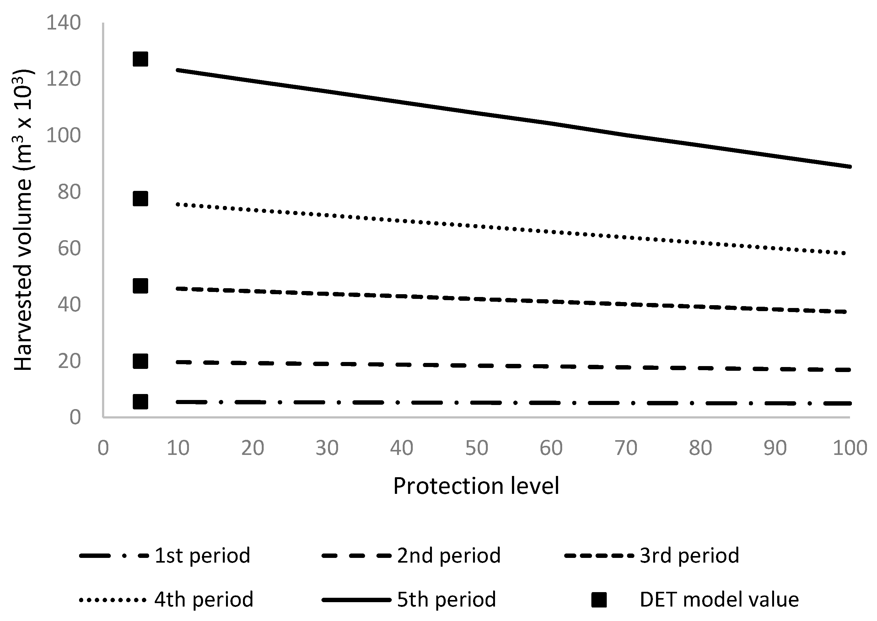
Figure 2.
The relation between the protection level and the harvested volume obtained by the robust (ROB) model (a) and simulation experiments (b) for each period.
Figure 2.
The relation between the protection level and the harvested volume obtained by the robust (ROB) model (a) and simulation experiments (b) for each period.

Table 1.
The periodic and total harvested volumes for different harvest flow percentages obtained using the DET model for 50% protection level in the first planning period (PP).
Table 1.
The periodic and total harvested volumes for different harvest flow percentages obtained using the DET model for 50% protection level in the first planning period (PP).
| Harvested Volume () | |||||||
|---|---|---|---|---|---|---|---|
| Period | Total | ||||||
| 1 | 2 | 3 | 4 | 5 | |||
| Harvest Flow Percentage (%) | 10 | 43,410 | 47,739 | 52,463 | 57,685 | 63,434 | 264,731 |
| 20 | 35,885 | 43,061 | 51,673 | 61,983 | 74,349 | 266,951 | |
| 30 | 29,764 | 38,692 | 50,279 | 65,323 | 84,876 | 268,934 | |
| 40 | 24,790 | 34,696 | 48,491 | 67,811 | 94,906 | 270,694 | |
| 50 | 20,713 | 30,996 | 46,492 | 69,635 | 104,426 | 272,262 | |
| 60 | 17,342 | 27,739 | 44,358 | 70,892 | 113,321 | 273,652 | |
| 70 | 14,600 | 24,814 | 42,164 | 71,633 | 121,674 | 274,885 | |
| 80 | 12,470 | 22,437 | 40,198 | 72,309 | 128,440 | 275,854 | |
| 90 | 11,118 | 21,083 | 40,048 | 75,891 | 128,046 | 276,186 | |
| 100 | 10,105 | 20,174 | 40,335 | 78,524 | 127,247 | 276,385 | |
| No harvest flow constraints | 5543 | 19,906 | 46,660 | 77,564 | 127,066 | 276,739 | |
Table 2.
The average periodic and total harvested volumes and their standard deviations for different harvest flow percentages obtained by simulation experiments for the DET model´s results for 50% protection level in the first PP.
Table 2.
The average periodic and total harvested volumes and their standard deviations for different harvest flow percentages obtained by simulation experiments for the DET model´s results for 50% protection level in the first PP.
| Harvested Volume () | |||||||
|---|---|---|---|---|---|---|---|
| Period | Total | ||||||
| 1 | 2 | 3 | 4 | 5 | |||
| Harvest flow percentage (%) | 10 | 41,244 ± 408 | 43,422 ± 738 | 45,048 ± 944 | 46,139 ± 1059 | 46,396 ± 1133 | 222,248 |
| 20 | 34,078 ± 421 | 39,161 ± 653 | 44,376 ± 928 | 49,685 ± 1180 | 54,217 ± 1079 | 221,517 | |
| 30 | 28,281 ± 292 | 35,208 ± 568 | 43,276 ± 896 | 52,334 ± 1204 | 61,929 ± 1402 | 221,027 | |
| 40 | 23,552 ± 282 | 31,593 ± 503 | 41,685 ± 908 | 54,309 ± 1184 | 69,185 ± 1428 | 220,324 | |
| 50 | 19,679 ± 249 | 28,201 ± 448 | 39,964 ± 863 | 55,748 ± 1207 | 76,196 ± 1492 | 219,789 | |
| 60 | 16,472 ± 201 | 25,240 ± 418 | 38,163 ± 849 | 56,816 ± 1302 | 82,642 ± 1445 | 219,333 | |
| 70 | 13,869 ± 156 | 22,603 ± 417 | 36,339 ± 750 | 57,251 ± 1241 | 88,628 ± 1579 | 218,690 | |
| 80 | 11,845 ± 164 | 20,408 ± 372 | 34,527 ± 772 | 57,917 ± 1151 | 93,655 ± 1568 | 218,353 | |
| 90 | 10,557 ± 173 | 19,188 ± 363 | 34,437 ± 755 | 60,806 ± 1182 | 93,340 ± 1609 | 218,327 | |
| 100 | 9597 ± 158 | 18,338 ± 340 | 34,667 ± 787 | 62,896 ± 1230 | 92,714 ± 1489 | 218,211 | |
| No harvest flow constraints | 5262 ± 108 | 18,408 ± 363 | 42,045 ± 920 | 67,879 ± 1539 | 107,904 ± 259 | 241,498 | |
Table 3.
The resulting gap tolerance for instances of the ROB model.
| Resulting Gap Tolerance (%) | |||||||
|---|---|---|---|---|---|---|---|
| The Protection Level (%) | |||||||
| 10 | 20 | 30 | 40 | 50 | 60 | ||
| Harvest flow percentage (%) | 10 | 0.00 | 0.00 | 0.00 | No Gap | No Gap | No Gap |
| 20 | 0.00 | 0.00 | 0.00 | No Gap | No Gap | No Gap | |
| 30 | No Gap | 0.00 | 0.00 | No Gap | No Gap | No Gap | |
| 40 | No Gap | No Gap | No Gap | No Gap | No Gap | No Gap | |
| 50 | 6.60 | 5.19 | 4.18 | 3.53 | 3.21 | 3.20 | |
| 60 | 4.42 | 3.07 | 2.29 | 0.92 | 0.43 | 0.16 | |
| 70 | 4.02 | 3.03 | 1.69 | 0.83 | 0.41 | 0.08 | |
| 80 | 4.17 | 2.89 | 1.67 | 0.86 | 0.37 | 0.02 | |
| 90 | 3.98 | 2.99 | 1.64 | 0.75 | 0.35 | 0.09 | |
| 100 | 3.81 | 2.75 | 1.55 | 0.84 | 0.37 | 0.08 | |
| No harvest flow constraints | 1.62 | 1.62 | 1.62 | 0.76 | 0.43 | 0.05 | |
Note: No gap indicates that solving the problem took longer than 1200 s without achieving the gap tolerance.
Table 4.
The real (achieved) harvest flow percentages for ROB models and simulations for 50% protection level in the first PP.
Table 4.
The real (achieved) harvest flow percentages for ROB models and simulations for 50% protection level in the first PP.
| ROB Model | Simulations | ||||||||
|---|---|---|---|---|---|---|---|---|---|
| Consecutive Periods | Consecutive Periods | ||||||||
| Protection Level | Harvest Flow | 1–2 | 2–3 | 3–4 | 4–5 | 1–2 | 2–3 | 3–4 | 4–5 |
| 50 | 50 | −36% | −35% | 21% | −34% | −34% | −44% | −48% | −37% |
| 50 | 60 | −36% | −35% | 18% | −34% | −34% | −34% | −60% | −51% |
| 50 | 70 | −36% | −35% | 16% | −34% | −34% | −35% | −56% | −65% |
| 50 | 80 | −33% | −32% | −29% | −31% | −31% | −21% | −9% | −2% |
| 50 | 90 | −44% | −44% | −42% | −43% | −43% | −33% | −22% | −10% |
| 50 | 100 | −41% | −41% | −39% | −39% | −39% | −45% | −35% | −24% |
Table 5.
The periodic and total harvested volumes for different harvest flow percentages obtained using the ROB model for 50% protection level in the first PP.
Table 5.
The periodic and total harvested volumes for different harvest flow percentages obtained using the ROB model for 50% protection level in the first PP.
| Harvested Volume () | |||||||
|---|---|---|---|---|---|---|---|
| Period | Total | ||||||
| 1 | 2 | 3 | 4 | 5 | |||
| Harvest flow percentage (%) | 50 | 69,005 | 46,287 | 35,404 | 30,980 | 23,450 | 205,126 |
| 60 | 87,437 | 48,583 | 31,436 | 23,593 | 20,447 | 211,496 | |
| 70 | 94,477 | 55,906 | 29,604 | 18,503 | 13,569 | 212,059 | |
| 80 | 93,959 | 59,997 | 32,395 | 16,198 | 9720 | 212,269 | |
| 90 | 93,765 | 59,730 | 37,691 | 14,459 | 6748 | 212,393 | |
| 100 | 93,800 | 59,795 | 37,554 | 15,942 | 5329 | 212,420 | |
| No harvest flow constraints | 92,898 | 59,677 | 38,919 | 16,461 | 4468 | 212,423 | |
Table 6.
The average periodic and total harvested volumes and their standard deviations of different harvest flow percentages obtained by simulation experiments for the ROB model´s results for 50% protection level in the first PP.
Table 6.
The average periodic and total harvested volumes and their standard deviations of different harvest flow percentages obtained by simulation experiments for the ROB model´s results for 50% protection level in the first PP.
| Harvested Volume () | |||||||
|---|---|---|---|---|---|---|---|
| Period | Total | ||||||
| 1 | 2 | 3 | 4 | 5 | |||
| Harvest flow percentage (%) | 50 | 73,644 ± 664 | 51,183 ± 728 | 40,771 ± 868 | 37,202 ± 1117 | 36,490 ± 1074 | 239,290 |
| 60 | 93,322 ± 726 | 53,825 ± 677 | 36,207 ± 801 | 28,318 ± 896 | 25,754 ± 1114 | 237,426 | |
| 70 | 100,876 ± 713 | 61,892 ± 817 | 34,089 ± 831 | 22,275 ± 686 | 17,074 ± 703 | 236,206 | |
| 80 | 100,289 ± 710 | 66,396 ± 857 | 37,290 ± 817 | 19,487 ± 664 | 12,240 ± 574 | 235,701 | |
| 90 | 100,063 ± 684 | 66,138 ± 805 | 43,440 ± 896 | 17,396 ± 611 | 8512 ± 446 | 235,548 | |
| 100 | 100,092 ± 725 | 66,160 ± 839 | 43,282 ± 876 | 19,143 ± 624 | 6706 ± 385 | 235,383 | |
| No harvest flow constraints | 99,148 ± 715 | 66,024 ± 843 | 44,925 ± 910 | 19,777 ± 632 | 5619 ± 369 | 235,493 | |
© 2017 by the authors. Licensee MDPI, Basel, Switzerland. This article is an open access article distributed under the terms and conditions of the Creative Commons Attribution (CC BY) license (http://creativecommons.org/licenses/by/4.0/).
Share and Cite
MDPI and ACS Style
Kašpar, J.; Hlavatý, R.; Kuželka, K.; Marušák, R. The Impact of Assumed Uncertainty on Long-Term Decisions in Forest Spatial Harvest Scheduling as a Part of Sustainable Development. Forests 2017, 8, 335. https://doi.org/10.3390/f8090335
AMA Style
Kašpar J, Hlavatý R, Kuželka K, Marušák R. The Impact of Assumed Uncertainty on Long-Term Decisions in Forest Spatial Harvest Scheduling as a Part of Sustainable Development. Forests. 2017; 8(9):335. https://doi.org/10.3390/f8090335
Chicago/Turabian StyleKašpar, Jan, Robert Hlavatý, Karel Kuželka, and Róbert Marušák. 2017. "The Impact of Assumed Uncertainty on Long-Term Decisions in Forest Spatial Harvest Scheduling as a Part of Sustainable Development" Forests 8, no. 9: 335. https://doi.org/10.3390/f8090335
Note that from the first issue of 2016, this journal uses article numbers instead of page numbers. See further details here.