Article

Carbon Emissions from Deforestation and Degradation in a Forest Reserve in Venezuela between 1990 and 2015

by
Carlos Pacheco-Angulo
1,*,
Emilio Vilanova
1,
Inmaculada Aguado
2,
Sergio Monjardin
3 and
Susana Martinez
2
1
Facultad de Ciencias Forestales y Ambientales, Universidad de los Andes, V-5101 Mérida, Venezuela
2
Departamento Geología, Geografía y Medio Ambiente, Universidad de Alcalá, E-28801 Madrid, España
3
Facultad deCiencias de la Tierra y el Espacio, Universidad Autónoma de Sinaloa, M-80029 Sinaloa, México
*
Author to whom correspondence should be addressed.
Forests 2017, 8(8), 291; https://doi.org/10.3390/f8080291
Submission received: 20 May 2017 / Revised: 4 August 2017 / Accepted: 10 August 2017 / Published: 11 August 2017

Abstract

:
This study presents for the first time in Venezuela a joint analysis of deforestation and forest degradation processes, including its effects on carbon emissions. The Caparo Forest Reserve, located in the Western Plains ecoregion, in one of the national hot spots of deforestation, served as a case study using three different periods: 1990–2000, 2000–2010 and 2010–2015. In the context of the United Nations Framework Convention on Climate Change (UNFCCC) framework, the Practice Guidance for Land Use, Land-Use Change and Forestry from the Intergovernmental Panel on Climate Change (IPCC) was followed. These guidelines combine the activity data for the estimation of deforestation and degradation rates, in this case using open access Landsat imagery in conjunction with the TerraAmazon system with the emission factors, and these based on aboveground biomass (AGB) estimations using field data from permanent plots monitored during the study period. Deforestation was responsible of a net loss of −53,461 ha, while close to −3667 ha were classified as degraded forests during the 1990–2000 decade (−4.9% annual deforestation rate). An estimated area of −36,447 ha and −515 ha between 2000 and 2010 was affected by both processes (−4.3% annual forest loss), and −8111 ha and −737 ha between 2010 and 2015 (−3.2% per year). These processes were responsible for an estimated equivalent in carbon emissions of 2.21 ± 0.32 (SEM—Standard Error of the Mean) Mt CO2 year−1 (1990–2000), 1.56 ± 0.19 Mt CO2per year between 2000 and 2010, while 0.80 ± 0.11 Mt CO2 year−1 during the 2010–2015 period. Between 92.9% and 98.63% (mean 94.9%) of these emissions came from deforestation, and between 1.37% and 7.79% (mean 5.1%) from forest degradation. Using available data, at national scale, deforestation and forest degradation in Caparo represented, on average, 0.49% of the total CO2 emissions and about 1.79% of land use change related emissions for the same period in Venezuela. Finally, we briefly outline a set of elements so these results can serve as a baseline for the potential establishment of a Reducing Emissions from Deforestation and Forest Degradation (REDD+) strategy in the area.

1. Introduction

Tropical forests cover an area close to 17.7 million km2 [1] comprising about 44% of the world’s forest area [2], and embody epicenters of biodiversity while playing a key role in the global climate system and for many other ecosystem services [3]. Despite this, and the recent efforts to control deforestation in some countries, the rate at which tropical forests are being replaced is still alarming and remains as a major concern [4,5]. It is estimated that 7.3 million ha were deforested annually in the 1990s and 3.3 million ha during the 2000–2015 period [2], mostly in the tropical region. The causes are diverse, with land use change for agriculture and livestock expansion and other development projects being the most important drivers of forest loss [6,7,8,9,10,11].
The loss of biodiversity is perhaps the most frequently addressed consequence of deforestation in tropical forests [12,13]. However, these ecosystems are also important reservoirs of carbon with averages between 200 and300 Mg C ha−1 in the aboveground biomass (AGB) [14]. Similarly, its function as important carbon sinks is well known, capturing about 15% of anthropogenic carbon emissions on a global scale [15,16]. Yet, deforestation and forest degradation processes are responsible for significant losses and reductions in carbon stocks [17,18,19,20,21]. On a global scale, using data from the FAO Forest Resource Assessment (FRA), Federici et al. [22] found an average rate of carbon emissions of 4.0 Gt CO2year−1 during the 2001–2010 decade, decreasing to an estimated rate of 2.9 Gt CO2 year−1 between 2011 and 2015 coming fundamentally from forest conversion. In the 2000s, carbon emissions coming from deforestation in the tropics were in the range of 0.6 to 1.2 Gt C year−1 [23,24,25]. Moreover, in a recent study focusing on the tropical and subtropical regions, Pearson et al. [21] estimated that, between 2005 and 2010, about 6.22 and 2.1 Gt CO2 were emitted every year from deforestation and forest degradation respectively. In this regard, it has been mentioned in the literature that these emissions are equivalent to 10–20% of total global carbon emissions [25,26,27,28,29].
The context of deforestation in Venezuela is not much different from other tropical countries. In an historical analysis, Pacheco et al. [30] found an average annual rate of forest loss of 0.30%, with a net decrease of 26.4% in the national forest cover between 1920 and 2008. It is during the 1950s when deforestation spiked mostly in the Western Plains ecoregion [31,32,33,34,35], which remained as one of the national hotspots of deforestation for a long time [36]. It has been shown that by the mid twentieth century, 36% of Venezuela’s forest cover was located to the north of the Orinoco River, and some estimates place this number to as low as 10% in recent decades [37]. Western plains have been mostly cleared for agricultural lands with current forests being mostly in protected areas and other areas with limited access. According to recent FAO estimates [1], 287,500 ha were lost every year in Venezuela between 1990 and 2000 (−0.6% year−1), with a decrease during the 2000–2010 decade of about 164,600 ha per year (−0.3%). More recently, these numbers were revisited by Hansen et al. [38], reporting, on average, 104,205 ha year−1 being lost due to deforestation between 2001 and 2015, and these estimates are being continuously monitored through the Global Forest Watch Initiative (GFW) (http://www.globalforestwatch.org). The main causes of deforestation in the country can be mostly attributed to agricultural expansion, development of infrastructure and selective logging with other associated indirect causes (see [9]) that are consistent with those found in many tropical areas [6,7,8,10].
The recent growth of global maps of forest carbon (e.g., [14,23,24,39]) offers the unique opportunity to compare these with other ground-based studies to have better estimates of the aboveground biomass and thus carbon in forests. For instance, available remote sensing data in Avitable et al. [39] show that Venezuelan forests can store between 65 and 480 Mg ha−1 in the AGB. Other field-based studies have also reported similar numbers by applying allometric equations to data collected on the ground. Using a series of permanent sample plots distributed throughout the country in five Venezuelan forest-types, Delaney et al. [40] reported AGB values from 140 Mg ha−1 in the very dry forests to 360 Mg ha−1 in the lowland moist forests of the Guiana Shield region.
The effects of deforestation and degradation in terms of carbon released have not been officially quantified at the national level. However, a few studies have shown that carbon emissions due to these processes can be significant. For example, between 1980 and 1990, Bonduki and Swisher [41] reported that up to 44% of the national CO2 emissions were caused by deforestation. Harris et al. [24] have shown that, between 2000 and 2005, about 9 Tg C year−1 (units are 1012 g of carbon per year) were lost due to deforestation in Venezuela. Other sources have estimated annual carbon emissions from deforestation in Venezuela adding up to between 9% [42] and 28% [38] of national emissions during the last decade. Furthermore, Pearson et al. [21] found that close to 10% of Venezuelan carbon emissions came from forest degradation between 2005 and 2010. In an attempt to quantify the carbon sink potential of Amazon forests between 1980 and 2010, Phillips and Brienen [43] estimated an average of 1 Tg C year−1 released through land use change activities for the Venezuelan Amazon region to the south of the Orinoco River. Interestingly, the net carbon uptake into mature forests (~8 Tg C year−1) exceeded the carbon emissions from land use change, but was considerably lower than the total fossil fuel emissions (~28 Tg C year−1) [43]. Combined, these results make a strong case for more in depth research about the national carbon budget and the implications of deforestation and forest degradation in it. The overall objective of this study was to analyze the deforestation and forest degradation processes, as well to estimate the associated carbon emissions in the Caparo Forest Reserve (CFR), an emblematic area of the Venezuelan Western Plains and a highly-threatened bioregion. For this, a combined approach of ground-based data and satellite imagery was used to jointly estimate the rates of deforestation and degradation and carbon emissions within the IPCC methodological framework for Land Use, Land-Use Change and Forestry (LULUCF) projects [44] and the Terra Amazon system [45]. CFR symbolizes the output of what occurred with forest cover throughout most of the Western Plains, a region with a complex socio-ecological system that has had a highly dynamic process of land use change in the last three decades. We focus our analysis in three different periods from 1990 to 2015 to have a comparative baseline with recent estimates of deforestation and degradation reported for the tropical region. Finally, we briefly discuss the potential implications of our findings in the context of the strategies for Reducing Emissions of Deforestation and Forest Degradation (REDD+).

2. Materials and Methods
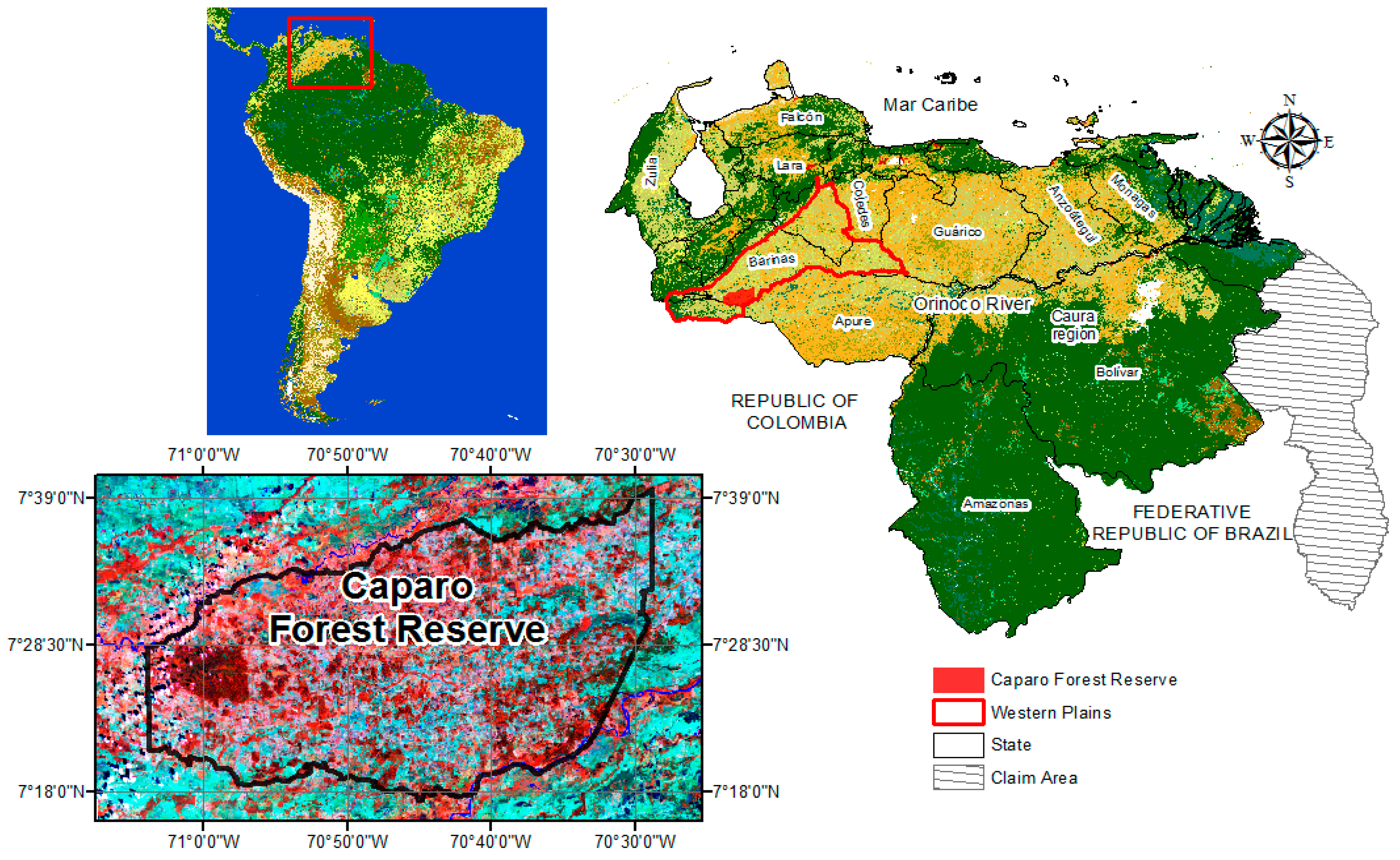
2.1. Study Area

Caparo Forest Reserve (CFR) is located in the Western Plains bioregion of Venezuela, to the southwest of Barinas State (Figure 1). Created as a protected zone in 1961 with an official area of 1744.84 km2, it was designated by law as an area with a timber management-oriented objective. It is located on a young alluvial flood plain with an altitude that varies from east to west from 120 to 140 m (Appendix A.1). The area is characterized by a tropical seasonal climate with two clear seasons (dry season from November to April; wet from May to October). The average annual rainfall is 2,156 mm with a mean annual average temperature is 24.9 °C [46].
The case of CFR is not unique within the Western Plains region of Venezuela. Timber concessions managed within a 25–30-year rotation cycle were established in the early 1970s and 1980s in the region. This includes three management units, in which access to timber was granted to six different private and mixed consortiums in CFR [47] (Appendix A.2). As in many other timber-managed areas in the tropics, selective logging was the primary activity which included road opening and the construction of temporary and permanent camps. Conventional logging practices in conjunction with significant timber volumes were fundamental causes of forest degradation with highly damaged residual stands in many areas [47]. For instance, Kammesheidt [48] found that up to 54% of the basal area was lost immediately after harvesting in some stands in the CFR, and after 19 years of logging some stands still remained under stocked compared to mature unlogged conditions.
Road construction for timber harvesting, along with a complex socio-economic environment seemed to have facilitated the subsequent agricultural colonization of the residual forests and other non-intervened forests in CFR [9]. According to Acevedo et al. [49], deforestation and degradation in the CFR occurred in an intricate sequence of stages that often started with selective logging followed by the burning of remaining forests mostly for subsistence activities. Later on, large portions of the area were completely transformed to cattle grazing farms in which land tenure was ultimately transferred to private owners contrary to official regulations [50,51]. Additional information about the causes of deforestation and degradation in this and other areas of the Western Plains and their socioeconomic implications can be found in Rojas [50,52].
Currently, CFR is primarily covered by grasslands, including areas with some legacy trees in a highly-fragmented landscape. In addition, riparian pockets of different forest types associated with permanent and/or semi-permanent streams and the Caparo River as the major watercourse can still be found in the area. Finally, an approximate section of 7,000 ha to the West of the reserve allocated to an experimental area with a research-oriented management remains as on the last relicts of the seasonal forests of the Western Plains bioregion [53], where close to one third of the area can be still be considered as a relatively mature old-growth forest with important implications for biodiversity conservation and other ecosystem services.
The methodological approach used in our study is based upon the guidelines proposed by the IPCC guide for good practices [17,44,55], which combines the Activity Data with the Emission Factors (EF). The first one refers to the estimation of deforestation and degradation rates using remote sensing tools, while the EF represent the estimation of carbon stocks and its corresponding emissions for the three periods considered here (1990–2000, 2000–2010 and 2010–2015), for which details are offered in the following sections.

2.2. Landsat Images

Images were acquired during the dry season (November–April) with about two-year difference from those established as references in our study (1990, 2000, 2010 and 2015). This is the same approach used in the FAO RSS project (Remote Sensing Survey) within the Forest Resources Assessment (FRA) program of 2015 [1]. These images correspond to the path 006 and row 55 selecting those with coordinates in the center of the image of latitude 7.2° and longitude −70.8°. Images were obtained from the USGS collection (U.S. Geological Survey) (http://glovis.usgs.gov/) and were taken on 20 January of 1988 (Landsat 4), 16 February 2001 (Landsat 5), 31 December 2009 (Landsat 7), and 2 February 2016 (Landsat 7), with the radiometric and geometric correction level L1T. For this analysis, the bands used were: red (0.63–0.69 μm), near infrared (0.76–0.90 μm) and medium infrared (1.55–1.75 μm).

2.3. Cartographic Criteria

We used the definition of forest based on the current Venezuelan Forest Law from 2008 [56], which specifies that in order to be considered a forest, any given area must have a minimum area of 0.5 ha, a tree canopy coverage of at least 30% and a minimum height of 5 m. For the CFR, this definition applies mostly to mature and secondary forests, riparian forests, “casildales” (small flooded areas highly dominated by Acacia articulate or “casildo” and forest plantations). Based on the guidelines of the UNFCCC, we define deforestation as the direct conversion, induced by man, of forested land into non-forest land [57]. Forest degradation is considered as a reduction in the capacity of a forest to produce ecosystem services such as carbon storage and wood products as a result of anthropogenic and environmental changes [58] caused by timber extraction activities, fire, cattle grazing in forest (both small and large scale) and/or an over exploitation of fire wood, charcoal or any other non-timber forest product [10,59]. This concept, although relatively easy to interpret, has proven to be challenging when trying to detect it using commonly-used remote sensing products, such as Landsat for any given area [21]. Given this complexity, we focused our attention exclusively on selective logging when estimating degradation rates. As shown by Asner et al. [60] in some areas of the Amazon, forest degradation from logging has been a precursor of deforestation and these activities can be detected using Landsat images. In our study area, logging has been a fundamental force of forest degradation for a great portion of the period considered here [49,50]. Finally, one hectare (1 ha) was assumed as the minimum mapping unit (MMU), with the years of analysis classified as follows: 1990 was defined as the baseline or Year 0, Year 2000 as Year 1, 2010 as Year 2, and 2015 as Year 3. As for the maps classes, these are composed of forests and non-forest areas for Year 0, while for Years 1, 2 and 3, degradation was added to the analysis.

2.4. Activity Data

2.4.1. Building the Map for Year 0 (1990)

To build the maps for our study period (1990, 2000, 2010 and 2015), the first step was the configuration of the TerraAmazon system, which consisted in a series of steps including the creation of the PostGres SQL database, defining the conceptual model, control access, control phase, the project, control rules, class definition, definition of control rules, and the definition of the area of interest [61]. Subsequently, to interpret and edit Year 0, a composition in false color with an RGB (453) was created, and a Linear Model of Spectral Mixtures approach was applied as proposed by Shimabukuro et al. [62]. From the spectral response of the Landsat bands, we estimated the proportion of the soil component, vegetation and shade for each pixel, resulting in images of the fragment soil, vegetation and shade (or water) by applying the following equation:
ri = a×vegetationi + b × soili + c × shadei + ei
where ri is the response of the pixel in the band i; a, b, and c are the proportions of vegetation, soil and shade (or water), respectively; vegetation, soil and shade are the spectral responses of the components of vegetation, soil and shade (or water); and ei is the error in the band i. Using the algorithm developed by the DPI-INPE (Image Processing Division—National Institute for Space Research) [63], a segmentation of the soil component was conducted since it provided the greater contrast between bare soil and forest. The latter is based on the “region growing” algorithm where a region is a set of homogeneous pixels connected based on their properties [64]. For its training, this algorithm requires two parameters: similarity, defined as the Euclidean distance between the mean digital numbers (here soil proportion) of two regions under which these are grouped together, and the minimum area to be considered as a region, defined by the number of pixels [65].
For this section, the parameters of the INPE’s Program for Deforestation Assessment in the Brazilian Legal Amazon (PRODES) were used: 8 as minimum criterion of similarity and 16 as minimum area value [66]. These segmentation values provided good results in a previous study on the same area [67]. The result of this segmentation was used for the visual interpretation process based on the approach of object based image analysis (OBIA) [68,69], which entailed assigning a thematic class of forest and non-forest to each object or region. To do this, composition 453 of Year 0 was used as background. Once this process was completed, we proceeded to back up the database and export the vector files in shape format for subsequent validations.

2.4.2. Building the Maps for Year 1 (2000), Year 2 (2010) and Year 3 (2015)

For creating the database of Year 1, the backup of Year 0 was restored, the image of Year 0 was deleted and the image of Year 1 was added. In addition, the topological rule “intersection” was added to interpret, specifically within the forest polygons of Year 0, the classes of deforestation and degradation of the forest at Year 1. To do this, two segmentations of the soil component (see Section 2.4.1) were retrieved from the image of Year 1: the first was used for the interpretation of deforestation which employs the values of the PRODES project applied earlier (see Section 2.4.1), and the second segmentation was used for the interpretation of forest degradation, using the values 4 as the minimum criterion of similarity and 8 as the minimum area value [70].
Deforestation under the OBIA approach was detected and identified on the image of Year 1 and within the forest of Year 0, and the segments or regions without forest were classified as deforestation for Year 1. Similarly, degradation was interpreted based upon the second segmentation, and in those areas within the forest of Year 0 where segments or regions were detected and identified. These included the main and secondary roads, as well as the logging yards, which were classified as forest degradation for Year 1. A similar approach was used for Years 2 and 3, considering that the forest classes of Year 1 and 2 were added correspondingly to the class of deforestation for the periods 2000–2010 and 2010–2015, and degradation for the years 2010 and 2015, respectively.

2.4.3. Estimation of the Average Annual Rate of Deforestation

We used the equation proposed by Sader [71] to estimate the rate of deforestation for our selected time periods:
Annual   Rate ( %   per   year ) = ( ( ( B 1 B 2 ) × 100 ) ( B 1 × N ) )
where B1 is the forest area on the initial date, B2 is the forest area on the final date and N is the number of years in the period.

2.4.4. Validation of Deforestation and Forest Degradation Maps

Once the forest and non-forest maps were created for Year 0, and the maps of deforestation and forest degradation for Years 1, 2 and 3 were produced, both processes were validated to provide robustness to the products and to assess the degree of agreement between the map and the ground-truth data [68,69,72]. Here, we used the methodology proposed by MacLean and Congalton [73] which generated area-based error matrices that can offer a better representation of the precision for maps created under the OBIA approach.
In order to make the sampling units directly comparable during validation, we used the objects or regions of the segmentations that were used earlier to generate the maps [69,74]. A stratified random sampling was applied as in Olofsson et al. [75], where each map class corresponded to a stratum (see more in Wulder et al. [76]), from which 50 objects were randomly selected and distributed throughout the area on the images that were used to generate the maps, as shown by Olofsson et al. [75] (Figure 2). This process was carried out by an external expert who did not intervene in the elaboration of maps [77]. As Chuvieco [72] noted, these ground-truth samples allowed us to achieve a higher precision by calculating the confusion matrix, and thus the errors of omission, commission and overall accuracy [69,72].

2.5. Emission Factors

2.5.1. Field Data

In some areas of the experimental unit of CFR, a set of permanent plots was established during the 1990s to monitor forest dynamics with an emphasis on turnover, growth and carbon cycle. The field plots in our study can be classified in two groups. The first one established between 1989 and 1990 and consist of 34 rectangular plots of 1000 m long by 10 m wide (1 ha transects) (Appendix A.3), systematically distributed trying to cover soil variations that are typical for alluvial systems [53]. The second group consist of six 0.25 ha plots (50 × 50 m) that were established between 1991 and 1996. In total, 40 plots have been periodically measured for all tree species including palms, with a stem diameter above 10 cm (see details in Appendix A.4). Approximately 90% of all individuals have been identified to the species level with the rest at least on a genus level. Based on the last census available for each plot, these forests have an average of 28.8 ± 2.4 m2 ha−1 (SEM) in basal area, and 288 ± 20 stems ha−1. The information about past disturbances and the history of the sites where plots were established is limited. However, there is no major evidence of any significant intervention, and these plots have been assumed to be representative of the mature forests that once covered the Western Plains region. Data collected from these plots were used here to estimate the aboveground biomass (see next Section) for the entire measurement period of each plot, although emphasis was placed on the reference dates of the satellite images and the periods considered here. Data for the second group of plots are included in the RAINFOR Project (www.rainfor.org), and are available through the forestplot.net portal [78,79].

2.5.2. Calculation of Coefficients

To estimate the coefficients that quantify carbon emissions caused by deforestation and forest degradation, we used the data from the plots described earlier. Upon the guidelines proposed by the Global Observation of Forest and Land Cover Dynamics panel (GOFC-GOLD) [59] for the establishment of REDD+ projects, we estimated the aboveground biomass (AGB) per tree in each plot and for each year of measurement using the allometric regression reported in Chave et al. [80] for tropical forests as follows:
(AGB) est = exp(−1.803 – 0.976E + 0.976 ln(ρ) + 2.673 ln(D) − 0.0299 (ln(D))2)
where AGB is the above-ground biomass of the tree expressed in kilograms (kg), E is a bioclimatic stress factor that has been shown to be an important covariate for the diameter-height relationships in tropical trees and includes information on temperature seasonality (TS) and a climatic water deficit (CWD) factor. Based on the geographical location of each plot, E and CWD were derived from a raster file below 2.5 arc-minute resolution available from http://chave.ups-tlse.fr/pantropical_allometry.htm (see more in Chave et al. [74] and in Appendix A.4); ρ is the stem wood density in gcm−3, with data assigned to every stem on a taxonomic basis from the pan-tropical database of Zanne et al. [81] and Chave et al. [82]. D is the diameter of every tree in cm. All estimations were performed on a plot basis and then scaled to 1 ha when needed. We assumed a 0.5 factor to transform AGB values into aboveground carbon (Mg C ha−1). The information was then analyzed to produce temporal trends on AGB and net biomass change over time. We estimated the net biomass change for each plot and for each period by subtracting the difference between AGB for the final and initial years of each period and divided by its length.
To estimate deforestation and degradation related emissions, several methods have been proposed with different challenges and advantages. In this study, we followed some of the insights provided by Baccini et al. [23] in the case of deforestation, and from Pearson et al. [21] for degradation. Here, we followed a more pragmatic approach where information derived from deforestation and degradation maps was directly linked to the field plot data in three ways.
(1)
Since deforestation and degradation rates were not estimated based on forest types, we assigned a global average AGB value to the forest class in the maps, while assuming a 100% loss of aboveground biomass for the non-forested areas.
(2)
Since our field plots are located in an undisturbed area, we used the studies of Kammesheidt [48], and Lozada et al. [53] as a baseline for the impact of logging on AGB in CFR managed forests. Per these, immediately after harvest, conventional logging can reduce 40–60% of the total basal area conditioned to several factors including logging intensity (number of trees harvested) and spatial distribution of commercial species. Since basal area is a good proxy for AGB we assumed an average of 50% reduction in AGB due to logging operations.
(3)
Once the aboveground carbon was estimated, using the standardized methodology described in WRI [51], we transformed these values to equivalent carbon dioxide emissions (CO2), multiplying the estimated amount of carbon (expressed in Mg C ha−1) by 44/12 which is the molecular weight ratio of carbon dioxide and the molecular weight of carbon (MgCO2 ha−1). To obtain the total amount of carbon emitted from deforestation and degradation, this value was multiplied by the estimated area of deforestation and forest degradation for each period.

3. Results and Discussion

3.1. Validation of Maps of Deforestation and Degradation

The results of the error matrices for each map are shown in Table 1. These are presented in terms of proportions of area as recommended by Olfsson et al. [75]. The row totals refers to the proportions of mapped area for each map, which represents each of the ground-truth samples in each class, which varied between 0.006334 and 0.008310. These variations are mostly a response of the variation in size of the segments used [69,83], although a proportional sampling of 50 segments per class was used.
On the other hand, column totals provide the proportions of the estimated area according to ground-truth data. For example, the estimated area of the forest class for the 1990 map is 0.003040. If we multiply this value by the total number of pixels in the map (1,935,538) the result is 5884 pixels or 530 ha, from which there was an agreement between the map and the ground-truth data of 5827 pixels or 524 ha, and an underestimation of 57 pixels or 5 ha, which were confused with the non-forest classes. In addition, based upon ground-truth data, the non-forest class can be interpreted as having an area of 6375 pixels or 574 ha, in which there was an agreement between the map and ground-truth data of 5978 pixels or 538 ha, while 397 pixels or 397 ha were confused with the forest class.
Deforestation class for the 2000 and 2015 maps and the non-forest class for the 2010 map were the categories with the highest agreement between the maps and the ground-truth data; conversely, degradation for the maps of 2000 and 2015, and the forest class for the map of 2010, were those with a higher confusion with the other classes.
The forest class, in the case of 1990 and 2000 maps, and the deforestation class for the 2010 and 2015 maps, had the largest commission errors generated by the user. A similar result was found for errors of omission, generated by the producer, where the non-forest class for the 1990 map and the degradation class for the 2000, 2010 and 2015 maps, had the largest errors. Meanwhile, estimated global precisions in all maps are within the limits established by similar studies when a differentiation of these categories is included (0.80 to 0.95) to evaluate their changes, as recommended by GOFC-GOLD [59] (Table 2).

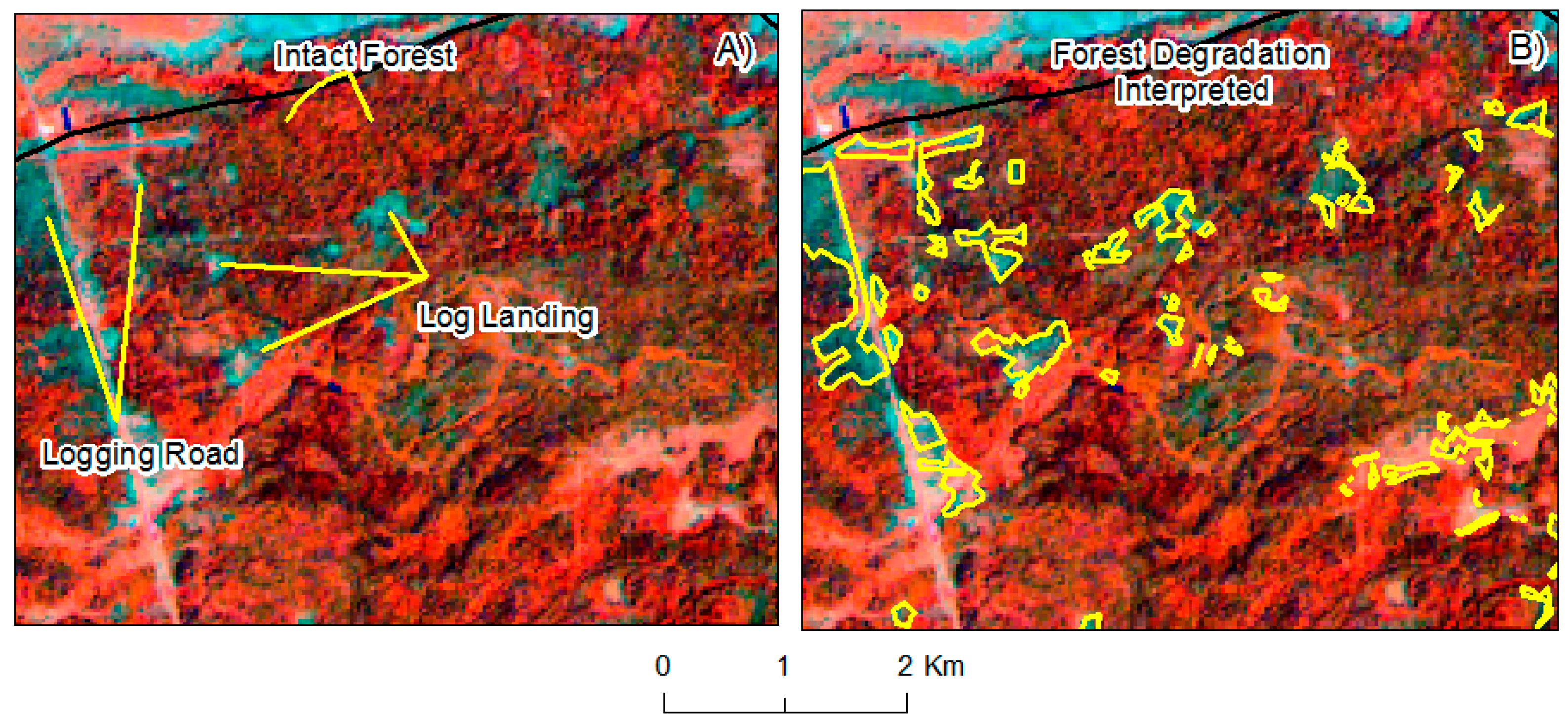
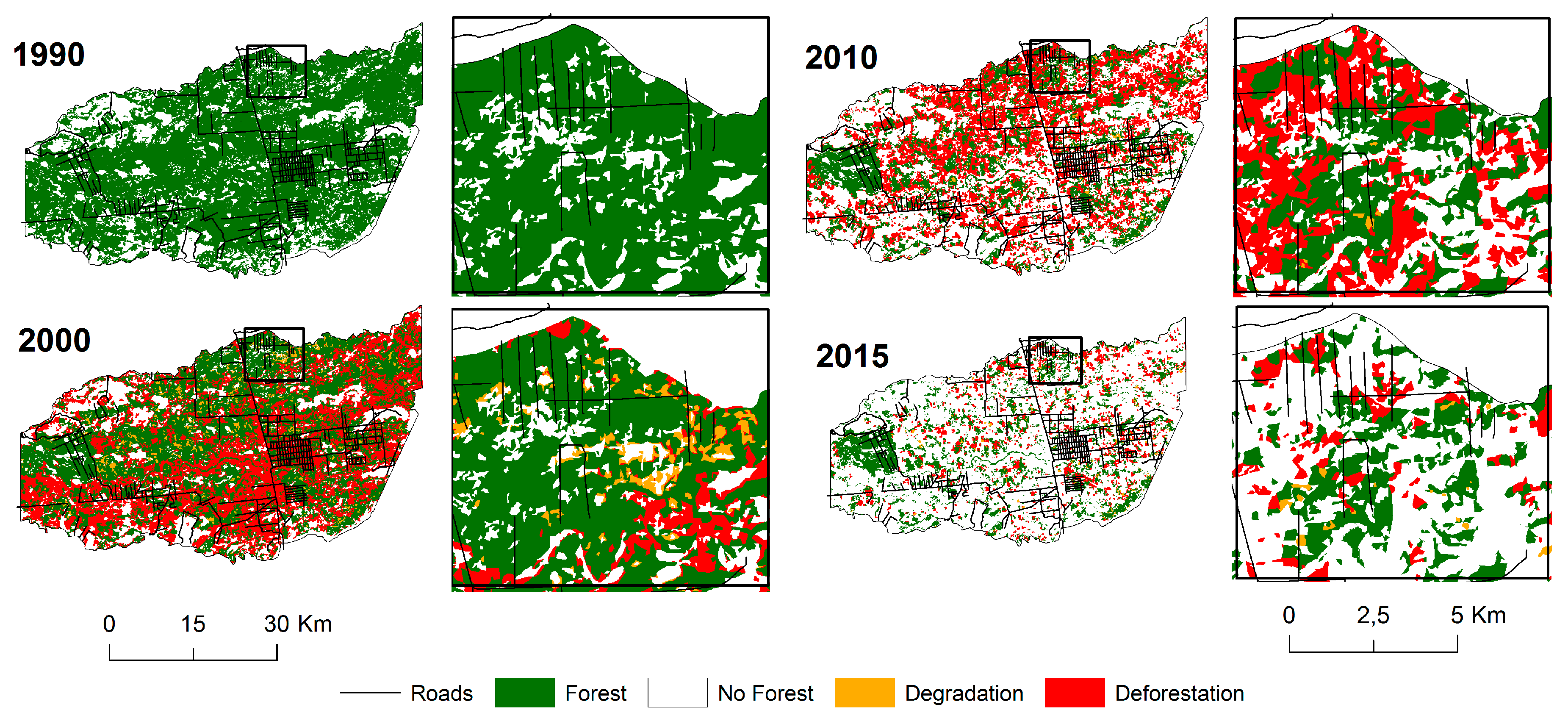
3.2. Cartography of Forests, Deforestation and Forest Degradation

Figure 3 shows the maps with the forest, non-forest, deforestation, and forest degradation classes. A continuous decrease in forest cover since 1990 is evident, and prevails throughout the entire period analyzed here, with the western region of the Caparo Experimental Station remaining mostly intact. The magnitude of this decline is evident when in 1990 CFR’s area was 77.28% covered by forests (134,612 ha), 44.39% (77,324 ha) in 2000, 22.85% (39,799 ha) in 2010, and 17.65% (30,749 ha) in 2015.
In terms of forest loss (red color in the map), deforestation during 1990–2000 (−53,461 ha) was much higher than the one found for 2000–2010 with −36,447 ha, and lower than during 2010–2015 with −8,111 ha. When the average annual deforestation rate was estimated, different trends were detected with the highest rate between 2000 and 2010 (−4.9% year−1), followed by the period 1990–2000 (−4.3% year−1) and −3.2% between 2010 and 2015. Accessibility was probably the major driver of these trends as deforestation in 1990–2000 was mostly towards the southern part of the reserve where major roads facilitated the colonization of San Camilo, another forest reserve to the south of Western Plains region [48,50]. Deforestation during 2000–2010 and 2010–2015 was mostly located towards the northern part of the CFR, where most of the remaining forests were located. Putting our results in perspective, deforestation in CFR was much higher than the annual national average of −0.30% year−1 as shown in Pacheco et al. [30] and in FRA 2015 [1]. Our results are also considerably higher than the annual average for the same area provided by the GFW for the last two periods: 2000–2010 with −1,327 ha year−1 (−1.5%) and 2010–2015 with −644 ha year−1 (−1.0%) [38].
Concerning forest degradation (orange color in the map), the highest proportion occurred during the 1990–2000 period with an approximate area of 3667 ha (2.10% of CFR’s area), followed by the 2010–2015 period with 0.42% (737 ha) and the 2000–2010 period with 0.30% (515 ha). These results are consistent with the history of forest management in the region where industrial logging operations were mostly halted after 1999 when a new form of community forestry was implemented [47,84]. As pointed out by Peres et al. [85], Landsat images can help detecting forest roads, collection yards and some areas with commercially harvested trees (logging gaps), which were the main drivers detected and interpreted as forest degradation in our study. As an example, some of these areas are shown in Figure 4 where forest degradation was identified for the 1990–2000 period.
If deforestation and forest degradation are analyzed at the same time, we see that 59% of the reserve was affected by both processes with approximately 102,938 ha in the 25 year-period of our study. Overall, 95.22% corresponded to deforestation and 4.78% to forest degradation. As expected, these percentages varied in the different periods considered here, with a range of 91.67% to 98.61% for deforestation and between 1.39% and 8.33% for forest degradation. As mentioned earlier, our estimates of forest degradation only considered those areas impacted by logging activities, and thus are likely to be an underestimation since other important drivers such as fires, cattle-grazing inside the forest or overexploitation of firewood and/or charcoal were not included.

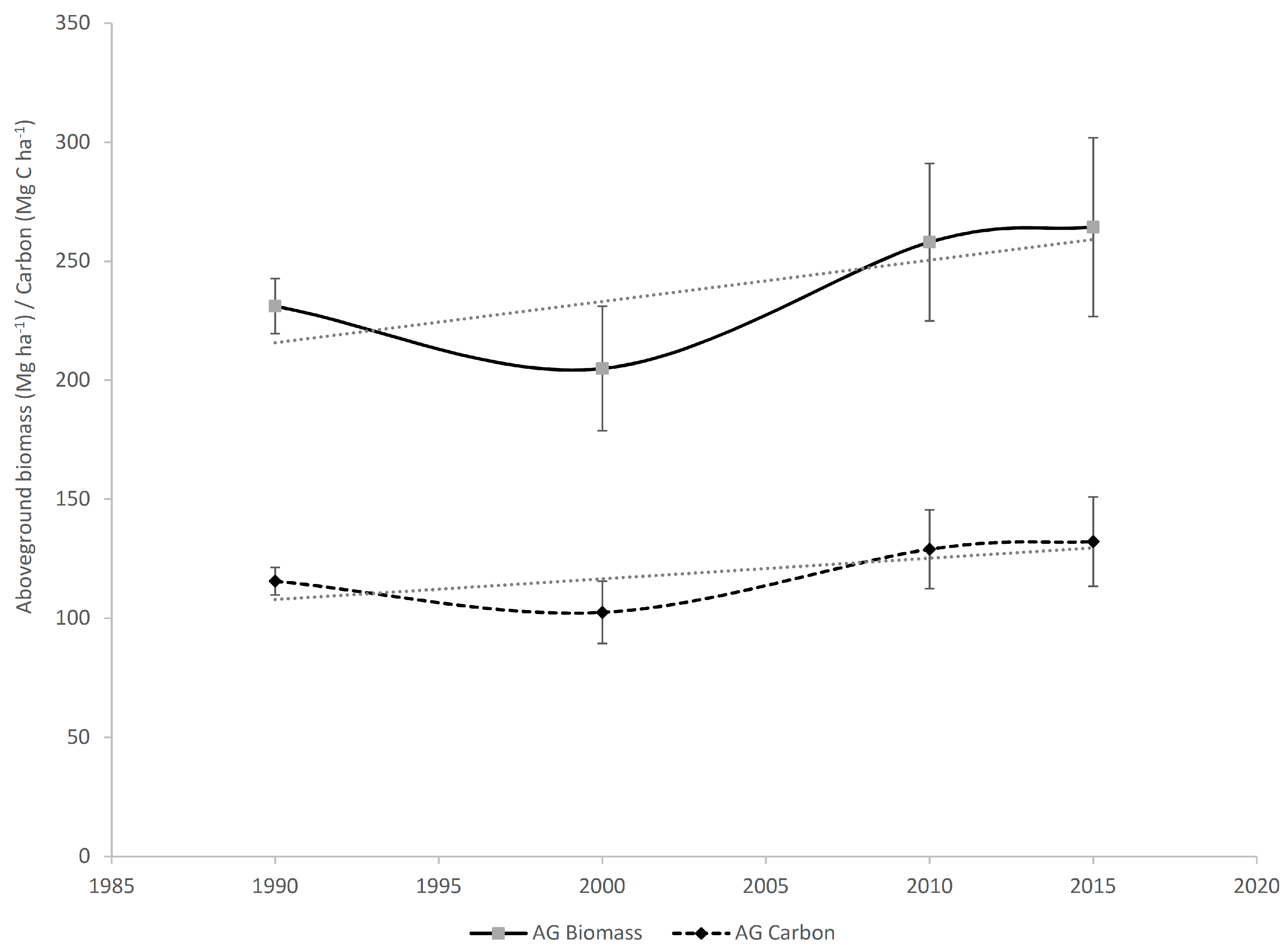
3.3. Estimation of Aboveground Biomass (AGB) and Carbon Emissions

The overall mean AGB for the entire period (239.60 ± 8.55 Mg ha−1—Standard Error of the Mean) is within the value found for this forest-type [40] but lower when compared to other more carbon-rich lowland moist forests of Venezuelan Guiana Shield [40,86,87]. The analysis of the net biomass change for the entire 1990–2015 period shows a carbon “sink” effect with 1.32 Mg ha−1 year−1 (+0.66 Mg C ha−1 year−1), a considerably higher rate than recent estimations made for the Amazon basin of 0.37 Mg C ha−1 year−1 during the 1980s and 1990s with a recent decline during 2000s for a rate of 0.24 Mg C ha−1 year−1 [43]. In Caparo, this dynamics seems to be consistent with the hypothesis of a changing ecology of tropical forests, where processes such as stem turnover has been increasing in the last few decades with an accelerated stem growth favoring a carbon sink effect [88]. Nevertheless, it is important to point out that alluvial terraces like those in the Western Plains region are highly influenced by nutrient-rich soils which tend to induce a much faster turnover compared to other sites [88] and thus a faster growth and carbon accumulation in the vegetation. In addition, historical records of Western plains show that these forests would be mostly composed by “young” communities that were developed after the region was affected by fires used for the establishment of livestock during the colonial period (1700–1810, i.e., the 19th century) and then later abandoned as a result of the independence wars [31,89]. The temporal trends in AGB and carbon from the permanent sample plots are shown in Figure 5.
During the period analyzed here, mean turnover rates were 1.4 to 4.3% year−1, in some cases doubling the rates reported for other Venezuelan forests [90]. Over the course of the last 25 years, recruitment dynamics positively favored the progressive incorporation of a greater number of individuals of the advanced regeneration to categories of larger size over time. Moreover, the large trees (>40 cm in diameter) accounted for almost 70% of the AGB in most of the plots, which is of great relevance when most logging operations in CFR have been highly selective mostly focusing on large individuals of a few commercial species that, combined with poor harvesting practices, have had a profound effect on the residual stand [47].
Although it appears to be a general trend towards increasing the amount of carbon stored in Caparo’s forests, tropical forests have shown to be highly sensitive to extreme drought phenomena, primarily related to an increase in the frequency of “Niño” years (ENSO). For example, during the extreme event of 2005 Amazonian drought, Phillips et al. [91] showed how many mature forest plots turned their dynamics from sinks to sources a few years after the drought event, due an unusual increase in the mortality of large trees affected by the reduction of water available in the ecosystem. In fact, a recent reanalysis of a large number of forest plots indicates a decline in the sink effect throughout the Amazon basin between 1980 and 2010 [92].
We used the mean AGB for each period to calculate the equivalent emissions from deforestation and forest degradation. An average value between the initial and final year of each period was used and these are shown in Table 3.
Our combined analysis shows that during the 1990–2000 decade more carbon was released than in any other of the other periods considered. The loss and degradation of about one third of the total CFR’s forested area during this period may have contributed to emit, on average, 2.21 Mt CO2 every year during this period. Depending on the period considered, forest degradation may have been responsible of about 0.7 to 4% of the total carbon emissions. As we see a decline in forest cover, it is obvious that less carbon was emitted in the subsequent periods (Table 4). However, the effects of deforestation in just one area may have had serious implications on a national scale. For instance, based on the most recent available data on carbon emissions [41], Venezuela emitted, on average, 307.98 ± 6.79 Mt CO2 year−1 between 1990 and 2013, from which 85.28 ± 9.34 (~28% of the total) came from deforestation and degradation. Despite the need for a higher precision in the estimation of carbon in the entire area of the reserve, we can conservatively assume that deforestation and degradation combined in CFR represented close to 0.49% of the total carbon emissions and 1.79% of those coming from deforested and degraded forests at national scale between 1990 and 2015.
The analysis of change in forest cover in the CFR shows that by 2015 the reserve still had an estimated area of forest of 30,749 ha (~18% of the total). Assuming a similar rate of deforestation from the 2010–2015 period of −3.2% per year, Venezuela could still be emitting a significant amount of carbon while also aggravating the current situation for biodiversity conservation in an extremely fragile ecosystem. A complete halt on deforestation and forest degradation in Caparo would allow to potentially maintain an estimated total of 27 Mt CO2 stored in these forests (expressed as the mean AGB scaled up to the area covered by forests).
Despite its obvious value, most of the available information on the variation of forest cover in Venezuela comes from studies at global or regional scales. In this regard, Pacheco et al. [30] have shown the limitations when estimating deforestation rates in Venezuela due to the lack of an official, continuous and systematic monitoring program of forest cover in the country. In addition, this study is, to our knowledge, the first attempt to jointly quantify carbon emissions and deforestation rates in Venezuela and therefore we cautiously call for taking the evidences presented here as preliminary. A more comprehensive analysis of carbon not only from forests but also from other vegetation types and/or land uses is needed. In any case, these results are intended to promote the application of the approach used here to other areas to collect baseline information on emissions of deforestation and forest degradation in Venezuela.

3.4. A Contribution to the Establishment of a REDD+ Strategy in the CFR

Our study shows how deforestation and forest degradation processes in the CFR have contributed in the last 25 years to the reduction of forest area in an important area of the Venezuelan Western plains. In addition, because of these processes, a high amount of carbon emissions was emitted. Although severely fragmented, the existence of a considerable area of forests and its associated stored carbon offers an opportunity to create a carbon-based initiative in the region. However, the continuous pressures to expand the agricultural frontier within the current national social and economic crisis are serious limitations that must be adequately assessed.
In the context of a strategy for Reducing Emissions from Deforestation and Forest Degradation (REDD+), multiple objectives can be managed simultaneously with the overall goal of creating economic incentives that can contribute to reduce deforestation and forest degradation, while attending its causes. One of the most critical steps implies obtaining reliable information on both deforestation and degradation rates and its associated carbon emissions. Our study partially aimed in this direction and tried to offer a pragmatic approach to take advantage of open access remote sensing data, an open source software (i.e., TerraAmazon) and the availability of long term field data. We believe that this approach can be expanded and used in combination with other available carbon maps that will allow for a more accurate estimation on the carbon stored in these forests.

4. Conclusions

For the first time in Venezuela, carbon emissions due to deforestation and forest degradation processes were estimated, with the overall goal of creating a baseline for a potential establishment of a REDD+ strategy in one of the most important hotspots of biodiversity and deforestation in the country. CFR represents an area that has undergone a severe process of forest loss and other ecosystem services over the last 25 years. We have applied an internationally recognized approach that allows for comparisons and that potentially could be expanded to other areas.
Our study provides evidence of the validity for the use, without any cost in the acquisition, of satellite images and related programs for their processing to conduct similar studies on how to estimate carbon emissions from deforestation and forest degradation in a seasonal tropical forest ecosystem. Of course, other associated costs mostly linked to the collection of long term data in the field can be significant. The use of the IPCC good practice guidelines with the recommendations of GOFC-GOLD is a good alternative for monitoring and estimating carbon.
An important aspect here is to emphasize that forest degradation, estimated through data from medium resolution sensors, proved to be challenging when compared to deforestation. An important limitation is that the spectral signature of the degraded forests changed after only two years, affected by the regrowth of vegetation and the rapid process of canopy closure, which often prevents the identification of some activities, such as selective logging, identification of burned areas, cattle grazing in forest or other degradation forces. However, the application of digital techniques to medium resolution data allowed us to detect activities of forest exploitation, including forest roads and logging yards that have been a major component of degradation in CFR. Finally, more studies are required to examine other digital techniques and thus determine which of them offers better results in these tropical environments.

Acknowledgments

Authors would like to thank two anonymous reviewers for their comments that helped improving the quality of the paper. The first author would like to thank the Universidad de Los Andes for the scholarship granted to carry out his PhD studies at the Universidad de Alcalá (UAH), Spain. Likewise, this work has been made possible by the support provided by the Department of Geography of the UAH during the period of doctoral training of C. Pacheco. Emilio Vilanova would like to acknowledge funding support from the RAINFOR network for fieldwork and data collection between 2009 and 2016. The RAINFOR forest monitoring network in Venezuela has been supported by the Natural Environment Research Council (grants NE/D005590/1 and NE/I028122/1) and the Gordon and Betty Moore Foundation. Special recognition to Julio Serrano and Pedro Salcedo and to all the staff at the Caparo Experimental Station for their collaboration in the field data collection.

Author Contributions

C.P. and I.A. designed the study; C.P. designed the methodology of the activity data in the TerraAmazon system; C.P. and S.M. downloaded and processed satellite images; S.M. validated the results of the activity data; E.V. collected part of the field data, processed and generated the emission factors; C.P., E.V., I.A. and S.M. analyzed and discussed the results; and C.P. wrote the manuscript. All authors performed the final review of the manuscript.

Conflicts of Interest

The authors declare no conflict of interest.

Appendix A

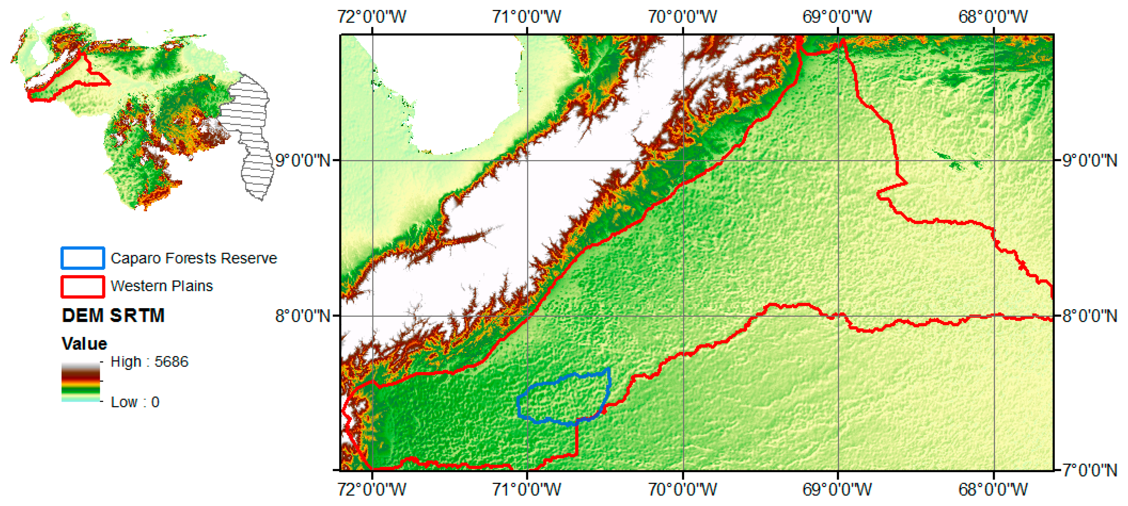
Appendix A.1. Digital Model Elevation (DEM)

Figure A1. Location of the study area within DME from NASA’s Shuttle Radar Topography Mission (SRTM) [93].
Forests 08 00291 g006

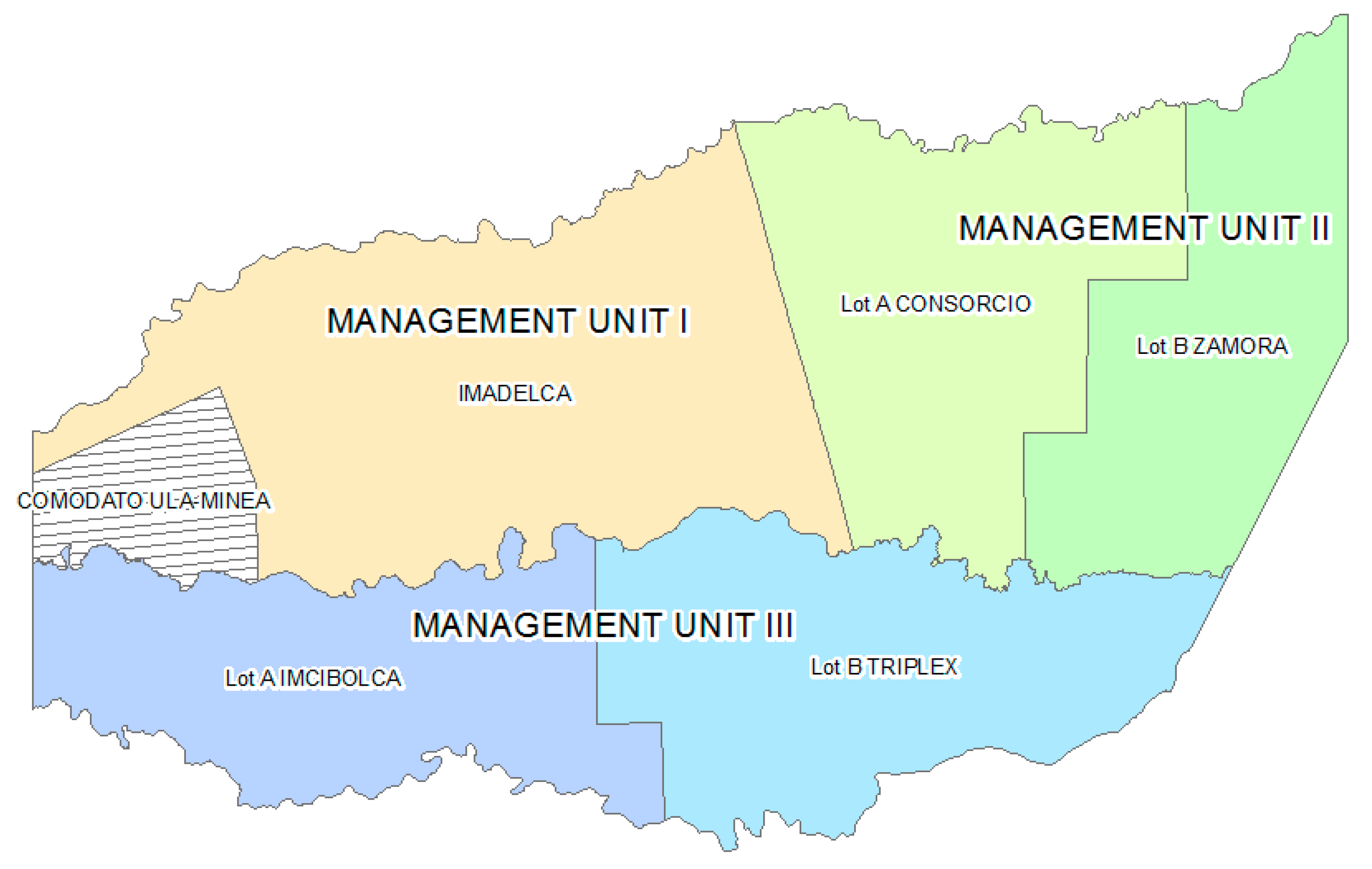
Appendix A.2. Caparo Forest Reserve (CFR) Management Units

Figure A2. Administrative management units listing the concessions allocated in the CFR.
Forests 08 00291 g007

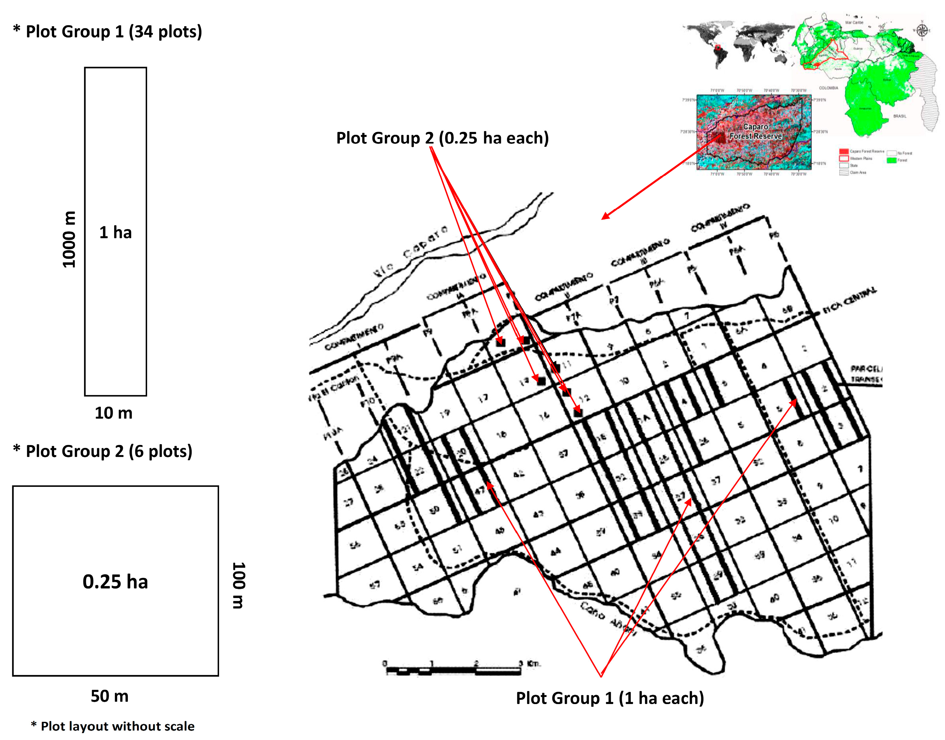
Appendix A.3. Location of Sample Plots

Figure A3. Location of permanent sample plots and general plot layout.
Forests 08 00291 g008

Appendix A.4. General Characteristic of the Plot Network Established in the Caparo Forest Reserve

Plot Code aPlot Area (ha)Minimum Dimension (m)Maximum Dimension (m)Altitude (masl)Climatic Water Deficit (CWD) bEnvironmental Stress Factor (E) bDate EstablishedLast Census DateMonitoring Period (years)No. of Censuses cInitial AGB (Mg ha−1) dFinal AGB (Mg ha−1) d
BAC-011101000132−427.6560.0451989.451995.385.936197.79191.93
BAC-021101000133−427.6560.0451989.451995.385.936224.81213.09
BAC-031101000135−427.6560.0451989.471995.385.906218.04214.62
BAC-041101000145−427.6560.0451989.471995.385.916189.37202.76
BAC-051101000148−427.6560.0451989.471993.253.795273.43279.74
BAC-061101000139−427.6560.0451989.471993.263.795363.03358.36
BAC-071101000141−427.6560.0451989.451995.385.936188.88211.88
BAC-081101000140−427.6560.0451989.451995.385.936260.58271.73
BAC-091101000145−427.6560.0451989.471995.385.916173.15195.38
BAC-101101000139−423.6610.0431989.432007.2017.7712373.33353.78
BAC-111101000137−423.6610.0431989.432007.2017.7712330.88348.56
BAC-121101000147−423.6610.0431989.442007.2017.7613271.24325.07
BAC-131101000141−423.6610.0431989.442007.2017.7613198.01256.59
BAC-141101000143−423.6610.0431989.431995.345.916116.49115.74
BAC-151101000146−423.6610.0431989.431995.375.956134.01133.29
BAC-161101000147−423.6610.0431989.431995.375.946142.57156.45
BAC-171101000142−423.6610.0431989.431995.375.956193.26214.34
BAC-181101000138−423.6610.0431989.431995.375.946354.06362.27
BAC-191101000144−423.6610.0431989.431995.375.956333.58336.09
BAC-201101000138−423.6610.0431989.411995.375.966181.46179.48
BAC-211101000142−423.6610.0431989.431995.375.956292.20306.91
BAC-221101000139−427.6560.0451989.441995.375.946159.26169.85
BAC-231101000138−427.6560.0451989.441995.345.906134.53131.32
BAC-241101000137−427.6560.0451989.432004.1214.687172.62243.28
BAC-251101000137.5−427.6560.0451989.442007.3117.8810252.86323.67
BAC-261101000137.0−427.6560.0451989.412009.3019.8914270.55345.76
BAC-271101000136−427.6560.0451989.412009.3119.9014266.66340.21
BAC-281101000136−427.6560.0451989.432009.4119.9814195.85147.65
BAC-291101000135−427.6560.0451989.432009.4119.9814141.22133.84
BAC-301101000135−427.6560.0451990.322007.1116.7911183.66173.85
BAC-311101000134−427.6560.0451990.322007.1116.7911197.52243.23
BAC-321101000134−427.6560.0451990.322007.1116.7811262.81249.93
BAC-331101000137−427.6560.0451990.322007.1116.7911298.86335.38
BAC-341101000139−427.6560.0451990.332006.1715.8410312.12324.15
BAC-350.255050141−427.6560.0451991.282016.3025.0213197.49219.75
BAC-360.255050143−427.6560.0451991.862016.3024.4412155.56205.68
BAC-370.255050144−427.6560.0451991.282016.3025.0210338.03422.12
BAC-380.255050138−427.6560.0451991.862016.3124.4512233.48259.65
BAC-390.255050142−423.6610.0432001.262016.3115.059124.39166.18
BAC-400.255050140−423.6610.0431996.312016.3120.0010283.97312.87
a The plot code refers to Barinas state (BA) and Caparo (C). b Number of census is the number of measurements or revisits to each plot. c Climate Water Deficit (CWD) and the Environmental Stress Factor (E) were extracted from a global climate layer for the long-term average of CWD and E at 2.5 arc-minute resolution as in Chave et al. [81]. d Initial and final AGB are based on the first and last census for each plot.

References

  1. Food and Agriculture Organization (FAO). Global Forest Resources Assessment 2015. Main Report; Food and Agriculture Organization of the UN: Rome, Italy, 2015. [Google Scholar]
  2. Keenan, R.; Reams, G.; Achard, F.; De Freitas, J.; Grainger, A.; Lindquist, E. Dynamics of global forest area: Results from the fao global forest resources assessment 2015. For. Ecol. Manag. 2015, 352, 9–20. [Google Scholar]
  3. Miura, S.; Amacher, M.; Hofer, T.; San-Miguel-Ayanz, J.; Ernawati; Thackway, R. Protective functions and ecosystem services of global forests in the past quarter-century. For. Ecol. Manag. 2015, 352, 35–46. [Google Scholar] [CrossRef]
  4. Lambin, E.F.; Turner, B.L.; Geist, H.J.; Agbola, S.B.; Angelsen, A.; Bruce, J.W.; Coomes, O.T.; Dirzo, R.; Fischer, G.; Folke, C.; et al. The causes of land-use and land-cover change: Moving beyond the myths. Glob. Environ. Chang. 2001, 11, 261–269. [Google Scholar] [CrossRef]
  5. Settele, J.; Scholes, R.; Betts, R.; Bunn, S.; Leadley, P.; Nepstad, D.; Overpeck, J.T.; Taboada, M.A. Terrestrial and inland water systems. In Climate Change 2014: Impacts, Adaptation, and Vulnerability. Part A: Global and Sectoral Aspects. Contribution of Working Group II to theFifth Assessment Report of the Intergovernmental Panel on Climate Change; Field, C.B., Barros, V.R., Dokken, D.J., Mach, K.J., Mastrandrea, M.D., Bilir, T.E., Chatterjee, M., Ebi, K.L., Estrada, Y.O., Genova, R.C., et al., Eds.; Cambridge University Press: Cambridge, UK; New York, NY, USA, 2014; pp. 271–359. [Google Scholar]
  6. Geist, H.; Lambin, E. Proximate cause and underlying driving forces of tropical deforestation. BioScience 2002, 52, 143–150. [Google Scholar] [CrossRef]
  7. Rudel, T.K.; Defries, R.; Asner, G.P.; Laurance, W.F. Changing drivers of deforestation and new opportunities for conservation. Conserv. Biol. 2009, 23, 1396–1405. [Google Scholar] [CrossRef] [PubMed]
  8. DeFries, R.S.; Rudel, T.; Uriarte, M.; Hansen, M. Deforestation driven by urban population growth and agricultural trade in the twenty-first century. Nat. Geosci. 2010, 3, 178–181. [Google Scholar] [CrossRef]
  9. Pacheco, C.; Aguado, I.; Mollicone, D. Las causas de la deforestación en Venezuela: Un estudio retrospectivo. Biollania 2011, 10, 281–292. [Google Scholar]
  10. Hosonuma, N.; Herold, M.; De Sy, V.; De Fries, R.; Brockhaus, M.; Verchot, L.; Angelsen, A.; Romijn, E. An assessment of deforestation and forest degradation drivers in developing countries. Environ. Res. Lett. 2012, 7, 044009. [Google Scholar] [CrossRef]
  11. Monjardín-Armenta, S.A.; Pacheco-Angulo, C.E.; Plata-Rocha, W.; Corrales-Barraza, G. La deforestación y sus factores causales en el estado de sinaloa, méxico. Madera y Bosques 2017, 23, 16. [Google Scholar] [CrossRef]
  12. Morales-Hidalgo, D.; Oswalt, S.N.; Somanathan, E. Status and trends in global primary forest, protected areas, and areas designated for conservation of biodiversity from the global forest resources assessment 2015. For. Ecol. Manag. 2015, 352, 68–77. [Google Scholar] [CrossRef]
  13. Barlow, J.; Lennox, G.D.; Ferreira, J.; Berenguer, E.; Lees, A.C.; Nally, R.M.; Thomson, J.R.; Ferraz, S.F.D.B.; Louzada, J.; Oliveira, V.H.F.; et al. Anthropogenic disturbance in tropical forests can double biodiversity loss from deforestation. Nature 2016, 535, 144–147. [Google Scholar] [CrossRef] [PubMed]
  14. Saatchi, S.S.; Harris, N.L.; Brown, S.; Lefsky, M.; Mitchard, E.T.A.; Salas, W.; Zutta, B.R.; Buermann, W.; Lewis, S.L.; Hagen, S.; et al. Benchmark map of forest carbon stocks in tropical regions across three continents. Proc. Natl. Acad. Sci. USA 2011, 108, 9899–9904. [Google Scholar] [CrossRef] [PubMed]
  15. Trumper, K.; Bertzky, M.; Dickson, B.; van Der Heijden, G.; Jenkins, P.; Manning, P. ¿La Solución Natural? El Papel de Los Ecosistemas en La Mitigación del Cambio Climático. Una Evaluación Rápida del Pnuma; Programa de las Naciones Unidas para el Medio Ambiente (PNUMA): Cambdrigde, UK, 2009; p. 39. [Google Scholar]
  16. Pan, Y.; Birdsey, R.A.; Fang, J.; Houghton, R.; Kauppi, P.E.; Kurz, W.A.; Phillips, O.L.; Shvidenko, A.; Lewis, S.L.; Canadell, J.G.; et al. A large and persistent carbon sink in the world’s forests. Science 2011, 333, 988–993. [Google Scholar] [CrossRef] [PubMed]
  17. Intergovernmental Panel on Climate Change(IPCC). Good Practice Guidance for Land Use, Land-Use Change and Forestry (Lulucf); Institute for Global Environmental Strategies: Hayama, Japan, 2003; p. 632. Available online: http://www.ipcc-nggip.iges.or.jp/public/gpglulucf/gpglulucf_files/GPG_LULUCF_FULL.pdf (accessed on 6 June 2016).
  18. Achard, F.; Stibig, H.J.; Eva, H.D.; Lindquist, E.J.; Bouvet, A.; Arino, O.; Mayaux, P. Estimating tropical deforestation from earth observation data. Carbon Manag. 2010, 1, 271–287. [Google Scholar] [CrossRef]
  19. Asner, G.P.; Powell, G.V.N.; Mascaro, J.; Knapp, D.E.; Clark, J.K.; Jacobson, J.; Kennedy-Bowdoin, T.; Balaji, A.; Paez-Acosta, G.; Victoria, E.; et al. High-resolution forest carbon stocks and emissions in the Amazon. Proc. Natl. Acad. Sci. USA 2010, 107, 16738–16742. [Google Scholar] [CrossRef] [PubMed]
  20. Bustamante, M.M.C.; Roitman, I.; Aide, T.M.; Alencar, A.; Anderson, L.O.; Aragão, L.; Asner, G.P.; Barlow, J.; Berenguer, E.; Chambers, J.; et al. Toward an integrated monitoring framework to assess the effects of tropical forest degradation and recovery on carbon stocks and biodiversity. Glob. Chang. Biol. 2016, 22, 92–109. [Google Scholar] [CrossRef] [PubMed]
  21. Pearson, T.R.H.; Brown, S.; Murray, L.; Sidman, G. Greenhouse gas emissions from tropical forest degradation: An underestimated source. Carbon Balance Manag. 2017, 12, 3. [Google Scholar] [CrossRef] [PubMed]
  22. Federici, S.; Tubiello, F.N.; Salvatore, M.; Jacobs, H.; Schmidhuber, J. New estimates of co2 forest emissions and removals: 1990–2015. For. Ecol. Manag. 2015, 352, 89–98. [Google Scholar] [CrossRef]
  23. Baccini, A.; Goetz, S.J.; Walker, W.S.; Laporte, N.T.; Sun, M.; Sulla-Menashe, D.; Hackler, J.; Beck, P.S.A.; Dubayah, R.; Friedl, M.A.; et al. Estimated carbon dioxide emissions from tropical deforestation improved by carbon-density maps. Nat. Clim. Chang. 2012, 2, 182–185. [Google Scholar] [CrossRef]
  24. Harris, N.L.; Brown, S.; Hagen, S.C.; Saatchi, S.S.; Petrova, S.; Salas, W.; Hansen, M.C.; Potapov, P.V.; Lotsch, A. Baseline map of carbon emissions from deforestation in tropical regions. Science 2012, 336, 1573–1576. [Google Scholar] [CrossRef] [PubMed]
  25. Achard, F.; Beuchle, R.; Mayaux, P.; Stibig, H.-J.; Bodart, C.; Brink, A.; Carboni, S.; Desclée, B.; Donnay, F.; Eva, H.D.; et al. Determination of tropical deforestation rates and related carbon losses from 1990 to 2010. Glob. Chang. Biol. 2014, 20, 2540–2554. [Google Scholar] [CrossRef] [PubMed]
  26. Intergovernmental Panel on Climate Change (IPCC). Cambio Climático 2007: Informe de Síntesis. Contribución de los Grupos de Trabajo I, II y III al Cuarto Informe de Evaluación del Grupo Intergubernamental de Expertos Sobre el Cambio Climático; Intergovernmental Panel on Climate Change: Ginebra, Suiza, 2007; p. 104. [Google Scholar]
  27. Houghton, R.A. How well do we know the flux of CO2 from land-use change? Tellus B 2010, 62, 337–351. [Google Scholar] [CrossRef]
  28. Kanninen, M.; Brockhaus, M.; Murdiyarso, D.; Nabuurs, G. Harnessing Forests for Climate Change Mitigation through REDD+; Series, I.W., Ed.; International Union of Forest Research Organizations (IUFRO): Vienna, Austria, 2010; Volume 25, pp. 43–54. [Google Scholar]
  29. Houghton, R.A.; House, J.I.; Pongratz, J.; van der Werf, G.R.; DeFries, R.S.; Hansen, M.C.; Le Quéré, C.; Ramankutty, N. Carbon emissions from land use and land-cover change. Biogeosciences 2012, 9, 5125–5142. [Google Scholar] [CrossRef]
  30. Pacheco, C.; Aguado, I.; Mollicone, D. Dinámica de la deforestación en Venezuela: Análisis de los cambios a partir de mapas históricos. Interciencia 2011, 36, 578–586. [Google Scholar]
  31. Veillón, J. Las Deforestaciones en los Llanos Occidentales de Venezuela Desde 1950 a 1975; Hamilton, L.S., Steyermark, J., Veillon, J.P., Mondolfi, E., Eds.; Conservación de los Bosques Húmedos de Venezuela: Caracas, Venezuela, 1977; pp. 97–110. [Google Scholar]
  32. Catalán, A. El Proceso de Deforestación en Venezuela Entre 1975–1988; Ministerio del Ambiente y de los Recursos Naturales Renovables: Caracas, Venezuela, 1992. [Google Scholar]
  33. Torres, A. La cuidada movilización de los recursos forestales. La industria forestal. Medio humano, establecimientos y actividades. In Geo Venezuela; Polar, F., Ed.; Tomo 3: Caracas, Venezuela, 2008; pp. 382–438. [Google Scholar]
  34. Guevara, J.; Carrero, O.; Costa, M.; Magallanes, A. Las selvas alisias: Hipótesis fitogeográfica para el área transicional del piedemonte andino y los altos llanos occidentales de Venezuela. Biollania 2011, 10, 178–188. [Google Scholar]
  35. Pacheco, C.; Vilanova, E. Dinámica de los cambios en la cobertura forestal en 27 municipios de los llanos occidentales de Venezuela (1990–2010). In Proceedings of Anais XVII Simpósio Brasileiro de Sensoriamento Remoto; INPE: João Pessoa-PB, Brazil, 2015; pp. 485–493. [Google Scholar]
  36. Pacheco, C.; Aguado, I.; Mollicone, D. Identification and characterization of deforestation hot spots in Venezuela using modis satellite images. Acta Amazon. 2014, 44, 185–196. [Google Scholar] [CrossRef]
  37. Torres-Lezama, A.; Ramírez-Angulo, H.; Vilanova, E.; Barros, R. Forest resources in Venezuela: Current status and prospects for sustainable management. Bois Forêts Tropiques 2008, 295, 21–33. [Google Scholar]
  38. Hansen, M.C.; Potapov, P.V.; Moore, R.; Hancher, M.; Turubanova, S.A.; Tyukavina, A.; Thau, D.; Stehman, S.V.; Goetz, S.J.; Loveland, T.R.; et al. Hansen/UMD/Google/USGS/NASA Tree Cover Loss and Gain Area. University of Maryland, Google, USGS, and NASA. 2013. Available online: www.globalforestwatch.org (accessed on 20 May 2017).
  39. Avitabile, V.; Herold, M.; Heuvelink, G.B.M.; Lewis, S.L.; Phillips, O.L.; Asner, G.P.; Armston, J.; Ashton, P.S.; Banin, L.; Bayol, N.; et al. An integrated pan-tropical biomass map using multiple reference datasets. Glob. Chang. Biol. 2016, 22, 1406–1420. [Google Scholar] [CrossRef] [PubMed] [Green Version]
  40. Delaney, M.; Brown, S.; Lugo, A.; Torres-Lezama, A.; Bello-Quintero, N. The distribution of organic carbon in major components of forests located in five life zones of Venezuela. J. Trop. Ecol. 1997, 13, 697–708. [Google Scholar] [CrossRef]
  41. Bonduki, Y.; Swisher, J. Options for mitigation greenhouse gas emissions in Venezuela’s forest sector: A general overview. Interciencia 1995, 20, 380–387. [Google Scholar]
  42. CAIT. Climate Data Explorer Institute. Available online: http://cait.wri.org (accessed on 2 June 2017).
  43. Phillips, O.L.; Brienen, R.J.W. Carbon uptake by mature amazon forests has mitigated amazon nations’ carbon emissions. Carbon Balance Manag. 2017, 12, 1. [Google Scholar] [CrossRef] [PubMed]
  44. Intergovernmental Panel on Climate Change (IPCC). Guidelines for National Greenhouse Gas Inventories—Volume 4, Agriculture, Land Use and Forestry (AFOLU); Intergovernmental Panel on Climate Change (IPCC): Ginebra, Suiza, 2006. [Google Scholar]
  45. TerraAmazon. Monitoring System of Deforestation in the Amazon; Fundação de Ciência, aplicações e Tecnologia Espacial and Instituto Nacional de Pesquisas Espaciais: São Jose dos Campos, Sao Paolo, Brazil, 2005. [Google Scholar]
  46. Maldonado, H. Análisis de la Deforestación en la Reserva Forestal Caparo-Venezuela, Períodos 1987–1994, 1994–2007 y 1987–2007; Universidad de Los Andes: Mérida, Venezuela, 2009. [Google Scholar]
  47. Kammesheidt, L.; Lezama, A.T.; Franco, W.; Plonczak, M. History of logging and silvicultural treatments in the western Venezuelan plain forests and the prospect for sustainable forest management. For. Ecol. Manag. 2001, 148, 1–20. [Google Scholar] [CrossRef]
  48. Kammesheidt, L. Stand structure and spatial pattern of commercial species in logged and unlogged Venezuelan forest. For. Ecol. Manag. 1998, 109, 163–174. [Google Scholar] [CrossRef]
  49. Acevedo, M.F.; Baird Callicott, J.; Monticino, M.; Lyons, D.; Palomino, J.; Rosales, J.; Delgado, L.; Ablan, M.; Davila, J.; Tonella, G.; et al. Models of natural and human dynamics in forest landscapes: Cross-site and cross-cultural synthesis. Geoforum 2008, 39, 846–866. [Google Scholar] [CrossRef]
  50. Rojas, J. La colonización agraria de las reservas forestales: ¿un proceso sin solución? Universidad de los andes, instituto de geografía, mérida, Venezuela. Cuadernos Geográficos 1993, 10, 110. [Google Scholar]
  51. World Resources Institute (WRI). The Greenhouse Gas Protocol: The Land Use, Land-Use Change, and Forestry Guidance for Ghg Project Accounting; World Resources Institute: Washington, DC, USA, 2005; p. 100. [Google Scholar]
  52. Rojas, J. La construcción geo-histórica de los llanos altos occidentales de Venezuela. Rev. Geogr. Venez. 2013, 54, 129–156. [Google Scholar]
  53. Lozada, J.R.; Arends, E.; Sánchez, D.; Villarreal, A.; Guevara, J.; Soriano, P.; Costa, M. Recovery after 25 years of the tree and palms species diversity on a selectively logged forest in a Venezuelan lowland ecosystem. For. Syst. 2016, 25, 1–12. [Google Scholar] [CrossRef]
  54. Bontemps, S.; Defourny, P.; van Bogaert, E. Globcover 2009 Products Description and Validation Report; European Space Agency (ESA) & The Université Catholique de Louvain: Louvain-la-Neuve, Belgium, 2010. [Google Scholar]
  55. Global Forest Observations Initiative (GFOI). Integrating Remote-Sensing and Ground-Based Observations for Estimation of Emissions and Removals of Greenhouse Gases in Forests: Methods and Guidance from the Global Forest Observation Initiative; Group on Earth Observations: Geneva, Switzerland, 2014; p. 190. [Google Scholar]
  56. Venezuela, R.B.D. Ley de bosques. In Decreto N° 6.070, de fecha 14/05/2008; Gaceta Oficial de la República Bolivariana de Venezuela. Nº 40.222, de fecha 06/08/2013; República Bolivariana de Venezuela: Caracas, Venezuela, 2013; p. 32. [Google Scholar]
  57. United Nations Framework Convention on Climate Change (UNFCCC). Decisions Adopted by cop16 (“the Cancun Agreements”) on Policy Approaches and Positive Incentives on Issues Relating to Reducing Emissions from Deforestation and Forest Degradation in Developing Countries; and the Role of Conservation, Sustainable Management of Forests and Enhancement of Forest Carbon Stocks in Developing Countries; UN-FCCC/CP/2010/7/Add.1 Decision 16/CMP.1., 231; UNFCCC: Bonn, Germany, 2011. [Google Scholar]
  58. Thompson, I.D.; Guariguata, M.R.; Okabe, K.; Bahamondez, C.; Nasi, R.; Heymell, V.; Sabogal, C. An operational framework for defining and monitoring forest degradation. Ecol. Soc. 2013, 18, 20. [Google Scholar] [CrossRef]
  59. Global Observation for Forest Cover and Land Dynamics (GOFC-GOLD). A Sourcebook of Methods and Procedures for Monitoring and Reporting Anthropogenic Greenhouse Gas Emissions and Removals Associated with Deforestation, Gains and Losses of Carbon Stocks in Forests Remaining Forests, and Forestation. GOFC-GOLD Report Version Cop22-1; GOFC-GOLD Land Cover Project Office, Wageningen University: Wageningen, The Netherlands, 2016. [Google Scholar]
  60. Asner, G.P.; Broadbent, E.N.; Oliveira, P.J.C.; Keller, M.; Knapp, D.E.; Silva, J.N.M. Condition and fate of logged forests in the brazilian amazon. Proc. Natl. Acad. Sci. USA 2006, 103, 12947–12950. [Google Scholar] [CrossRef] [PubMed]
  61. Instituto Nacional de Pesquisas Espaciais-Fundação de Ciência, Aplicações e Tecnologia Espaciais (INPE-FUNCATE). Terraamazon 4.4 User´s Guide Administrator; INPE FUNCATE: São Jose dos Campos, Sao Paolo, Brasil, 2013; p. 156. [Google Scholar]
  62. Shimabukuro, Y.E.; Smith, J.A. The least-squares mixing models to generate fraction images derived from remote sensing multispectral data. IEEE Trans. Geosci. Remote Sens. 1991, 29, 16–20. [Google Scholar] [CrossRef]
  63. Câmara, G.; Souza, R.C.M.; Freitas, U.M.; Garrido, J. Spring: Integrating remote sensing and gis by object-oriented data modelling. Comput. Grphic. 1996, 20, 395–403. [Google Scholar] [CrossRef]
  64. Zucker, S.W. Region growing: Childhood and adolescence. Comput. Graphic. Image Proc. 1976, 5, 382–399. [Google Scholar] [CrossRef]
  65. Shimabukuro, Y.E.; Batista, G.T.; Mello, E.M.K.; Moreira, J.C.; Duarte, V. Using shade fraction image segmentation to evaluate deforestation in landsat thematic mapper images of the Amazon region. Int. J. Remote Sens. 1998, 19, 535–541. [Google Scholar] [CrossRef]
  66. Instituto Nacional de Pesquisas Espaciais (INPE). Monitoring of the Brazilian Amazonian: Projeto Prodes National Space Agency of Brazil ed.; Instituto Nacional de Pesquisas Espaciais (INPE): São Jose dos Campos, Sao Paolo, Brasil, 2013. [Google Scholar]
  67. Pacheco, C.; Aguado, I.; Lopez, J. Comparación de los métodos utilizados en el monitoreo de la deforestación tropical, para la implementación de estrategias REDD+, caso de estudio los llanos occidentales Venezolanos. In Proceedings of Anais XVI Simpósio Brasileiro de Sensoriamento Remoto—SBSR; INPE: Foz do Iguaçu, Brazil, 2013; pp. 2817–2826. [Google Scholar]
  68. Jensen, J.R. Introductory Digital Image Processing: A Remote Sensing Perspective, 3rd ed.; Prentice-Hall: Upper Saddle River, NJ, USA, 2005; p. 323. [Google Scholar]
  69. Congalton, R.; Green, K. Assesing the Accuracy of Remotely Sensed Data: Principles and Practices; Taylor and Francis Group: London, UK; CRC Press: New York, NY, USA, 2009. [Google Scholar]
  70. Bins, S.A.; Fonseca, L.M.G.; Erthal, G.J.; Li, M. Satellite imagery segmentation: A region growing approach. In Proceedings of Anais Do VII Simpósio Brasileiro de Sensoriamento Remoto; INPE: Salvador, Brazil, 1993. [Google Scholar]
  71. Sader, A. Deforestation rates and trends in costa rica, 1940 to 1983. Biotropica 1988, 20, 11–19. [Google Scholar] [CrossRef]
  72. Chuvieco, E. Teledetección Ambiental. La Observación de la Tierra Desde el Espacio; Editorial Ariel, S.A.: Madrid, España, 2008; p. 430. [Google Scholar]
  73. MacLean, M.; Congalton, R. Map accuracy assesment issues when using an object-oriented approach. In Proceedings of the ASPRS 2012 Annual Conference—American Society for Photogrammetry and Remote Sensing, Sacramento, CA, USA, 19–23 March 2012. unpaginated CD-ROM. [Google Scholar]
  74. Radoux, J.; Bogaert, P.; Fasbender, D.; Defourny, P. Thematic accuracy assessment of geographic object-based image classification. Int. J. Geogr. Inf. Sci. 2011, 25, 895–911. [Google Scholar] [CrossRef]
  75. Olofsson, P.; Foody, G.M.; Herold, M.; Stehman, S.V.; Woodcock, C.E.; Wulder, M.A. Good practices for estimating area and assessing accuracy of land change. Remote Sens. Environ. 2014, 148, 42–57. [Google Scholar] [CrossRef]
  76. Wulder, M.A.; White, J.C.; Magnussen, S.; McDonald, S. Validation of a large area land cover product using purpose-acquired airborne video. Remote Sens. Environ. 2007, 106, 480–491. [Google Scholar] [CrossRef]
  77. Congalton, R. Comparison of sampling schemes used in generating error matrices for assessing the accuracy of maps generated from remotely sensed data. Photogramm. Eng. Remote Sens. 1988, 54, 593–600. [Google Scholar]
  78. Lopez-Gonzalez, G.; Lewis, S.L.; Burkitt, M.; Phillips, O.L. Forestplots.Net: A web application and research tool to manage and analyse tropical forest plot data. J. Veg. Sci. 2011, 22, 610–613. [Google Scholar] [CrossRef]
  79. Lopez-Gonzalez, G.; Lewis, S.L.; Burkitt, M.; Baker, T.R.; Phillips, O.L. Forestplots. Net Database (04/17). Available online: www.forestplots.net (accessed on 2 June 2017).
  80. Chave, J.; Réjou-Méchain, M.; Búrquez, A.; Chidumayo, E.; Colgan, M.S.; Delitti, W.B.C.; Duque, A.; Eid, T.; Fearnside, P.M.; Goodman, R.C.; et al. Improved allometric models to estimate the aboveground biomass of tropical trees. Glob. Chang. Biol. 2014, 20, 3177–3190. [Google Scholar] [CrossRef] [PubMed]
  81. Zanne, A.E.; Lopez-Gonzalez, G.; Coomes, D.A.; Ilic, J.; Jansen, S.; Lewis, S.L.; Miller, R.B.; Swenson, N.G.; Wiemann, M.C.; Chave, J. Data from: Towards a worldwide wood economics spectrum. Dryad Data Repository. Ecol. Lett. 2009. [Google Scholar] [CrossRef]
  82. Chave, J.; Coomes, D.; Jansen, S.; Lewis, S.L.; Swenson, N.G.; Zanne, A.E. Towards a worldwide wood economics spectrum. Ecol. Lett. 2009, 12, 351–366. [Google Scholar] [CrossRef] [PubMed]
  83. Desclée, B.; Bogaert, P.; Defourny, P. Forest change detection by statistical object-based method. Remote Sens. Environ. 2006, 102, 1–11. [Google Scholar] [CrossRef]
  84. Lozada, R. Situación actual y perspectivas del manejo de recursos forestales en Venezuela. Rev. For. Venez. 2007, 51, 195–218. [Google Scholar]
  85. Peres, C.A.; Barlow, J.; Laurance, W.F. Detecting anthropogenic disturbance in tropical forests. Trends Ecol. Evol. (Pers. Ed.) 2006, 21, 227–229. [Google Scholar] [CrossRef] [PubMed]
  86. Malhi, Y.; Wood, D.; Baker, T.R.; Wright, J.; Phillips, O.L.; Cochrane, T.; Meir, P.; Chave, J.; Almeida, S.; Arroyo, L.; et al. The regional variation of aboveground live biomass in old-growth amazonian forests. Glob. Chang. Biol. 2006, 12, 1107–1138. [Google Scholar] [CrossRef]
  87. Vilanova, E.; Ramírez-Angulo, H.; Torres-Lezama, A. El almacenamiento de carbono en la biomasa aérea como un indicador del impacto de la extracción selectiva de maderas en la reserva forestal imataca, Venezuela. Interciencia 2010, 35, 659–665. [Google Scholar]
  88. Phillips, O.; Higuchi, N.; Vieira, S.; Baker, T.; Chao, K.; Lewis, S. Changes in amazonian forest biomass, dynamics, and composition, 1980–2002. Amazonia and global change. Geophys. Monogr. Ser. 2009, 186, 373–387. [Google Scholar]
  89. Ramírez, H.; Acevedo, M.; Ataroff, M.; Torres-Lezama, A. Adaptación de un modelo de claros para el estudio de la dinámica de un bosque estacional en los llanos occidentales de Venezuela. Rev. For. Venez. 2010, 54, 207–226. [Google Scholar]
  90. Ramírez-Angulo, H.; Torres-Lezama, A.; Serrano, J. Mortalidad y reclutamiento de árboles en un bosque nublado de la cordillera de los andes, Venezuela. Ecotropicos 2002, 15, 177–184. [Google Scholar]
  91. Phillips, O.L.; van der Heijden, G.; Lewis, S.L.; López-González, G.; Aragão, L.E.O.C.; Lloyd, J.; Malhi, Y.; Monteagudo, A.; Almeida, S.; Dávila, E.A. Drought mortality relationships for tropical forests. New Phytol. 2010, 187, 631–646. [Google Scholar] [CrossRef] [PubMed] [Green Version]
  92. Brienen, R.J.; Phillips, O.L.; Feldpausch, T.R.; Gloor, E.; Baker, T.R.; Lloyd, J.; Lopez-Gonzalez, G.; Monteagudo-Mendoza, A.; Malhi, Y.; Lewis, S.L.; et al. Long-term decline of the Amazon carbon sink. Nature 2015, 519, 344. [Google Scholar] [CrossRef] [PubMed] [Green Version]
  93. Farr, T.G.; Rosen, P.A.; Caro, E.; Crippen, R.; Duren, R.; Hensley, S.; Kobrick, M.; Paller, M.; Rodriguez, E.; Roth, L.; et al. The shuttle radar topography mission. Rev. Geophys. 2007, 45. [Google Scholar] [CrossRef]
Figure 1. Location of the Caparo Forest Reserve (CFR), highlighting South America, Venezuela and the Western Plains bioregion on the map Globcover map of 2009 [54]. The CFR is shown in a Landsat Image of 2011 (RGB: 453) on bottom left corner. Dark-red areas correspond to the forests, while light red to crops and grasses, and cyan to bare soils.
Forests 08 00291 g001
Figure 2. Distribution of sampling objects or region based on a stratified random approach, here applied to the 2000 image.
Forests 08 00291 g002
Figure 3. Maps of forest cover, deforestation and forest degradation in the Caparo Forest Reserve between 1990 and 2015.
Forests 08 00291 g003
Figure 4. Detection of forest roads, logging yards and intact forests (A); and interpretation of forest degradation (B) for the 1990–2000 period in a 2000 Landsat image.
Forests 08 00291 g004
Figure 5. Temporal dynamics of AGB (solid lines) and carbon (dashed line) in the CFR forests. The carbon corresponds to 50% of AGB. Bars indicate the standard error or the mean for each year. A general linear trend is provided.
Forests 08 00291 g005
Table 1. Error matrix in terms of estimated proportions of area for each map maps.
ClassesGround-Truth (%)
19902000
ForestNon-ForestDeforestationDegradationTotalForestNon-ForestDeforestationDegradationTotal
Forest0.0030110.000205--0.0032160.0013170.0000290.0000600.0001100.001516
Non-Forest0.0000290.003089--0.0031180.0000530.0017920.0000280.0000140.001887
Deforestation-----0.0000360.0000710.0019540.0000620.002122
Degradation-----0.0000040.00000800.0012390.001251
Total0.0030400.003294--0.0063340.0014100.0019000.0020420.0014250.006776
20102015
ForestNon-ForestDeforestationDegradationTotalForestNon-ForestDeforestationDegradationTotal
Forest0.0035770.0000060.0000450.0000500.0036790.0026280.0000400.0000300.0000450.002742
Non-Forest0.0001070.0024160.0000790.0000190.0026210.0000560.0036630.0000190.0000120.003749
Deforestation0.0001440.0000180.0014380.0000190.0016180.0000070.0000210.0010000.0000480.001075
Degradation0.000012000.0003800.0003920.000001000.0006380.000639
Total0.0038400.0024400.0015610.0004680.0083100.0026920.0037230.0010490.0007420.008206
Table 2. Reliability indices of deforestation and forest degradation in terms of estimated proportions of area.
Maps
Error (%)1990200020102015
ForestCommission0.07060.13120.02760.0417
Omission0.00940.0660.06870.0239
Non-ForestCommission0.00850.05060.07820.0231
Omission0.06430.05680.01010.0162
DegradationCommission 0.07940.11160.0699
Omission 0.0430.07890.0463
DeforestationCommission 0.00950.03160.002
Omission 0.13050.18870.1406
Global precision (%)0.96100.92990.93990.9662
Table 3. Baseline values of biomass, carbon and equivalents for the calculation of emissions (including standard error or the mean).
YearBiomass (Mg ha−1)Carbon (Mg C ha−1)CO2 Equivalent (Mg CO2 ha−1)
1990231.14 ± 11.59115.57 ± 5.79423.76 ± 21.26
2000204.91 ± 26.15102.45 ± 13.08375.66 ± 47.94
2010257.99 ± 33.05128.99 ± 16.52472.98 ± 60.59
2015264.38 ± 37.56132.19 ± 18.78484.68 ± 68.87
Table 4. Estimated emissions from deforestation and forest degradation in the Caparo Forest Reserve between 1990 and 2015. Values in parenthesis are standard error of the mean.
Emissions per Period (Mt CO2 year−1)
1990–20002000–20102010–2015
Deforestation2.14 (0.18)1.55 (0.19)0.77 (0.11)
Degradation0.07 (0.01)0.01 (0.001)0.03 (0.004)
Total2.21 (0.19)1.56 (0.19)0.8 (0.11)

