Article

Quantification of Phosphorus Exports from a Small Forested Headwater-Catchment in the Eastern Ore Mountains, Germany

Institute of Soil Science and Site Ecology, TU Dresden, Pienner Str. 19, 01737 Tharandt, Germany
*
Author to whom correspondence should be addressed.
Forests 2017, 8(6), 206; https://doi.org/10.3390/f8060206
Submission received: 13 April 2017 / Revised: 4 June 2017 / Accepted: 7 June 2017 / Published: 10 June 2017

Abstract

:
Phosphorus (P) export from forest soils is mainly driven by storm events, which induce rapid flow processes by preferential flow bypassing large parts of the soil matrix. However, little is known about the dynamics, magnitude, and driving processes of P exports into surface waters. In this paper, we present the results of a monitoring study in a small forested catchment (21 ha) situated in the low mountain ranges of Saxony, Germany. During the fixed schedule-sampling (weekly to bi-weekly sampling frequency for a three-year period), a mean total-P concentration of 8 μg·L−1 was measured. However, concentrations increased up to 203 μg·L−1 during individual storm flow events. Based on the analyzed concentrations and continuously measured discharge we calculated mean annual export rates of 19 to 44 g·ha−1·a−1 for the weekly sampling frequency with different load calculation methods. If events are included into the annual load calculation, the mean annual export fluxes can be up to 83 g·ha−1·a−1 based on the different load calculation methods. Predictions of total-P export rates based on a sampling strategy which does not consider short-term changes due to factors such as storms will substantially underestimate P exports.

1. Introduction

Phosphorus (P) is an important element in the nutrition of forest ecosystems [1,2]. At the landscape scale, P is exported mainly via streamflow either in solution or as a particulate, and in either organic or inorganic forms [3,4,5]. The magnitude and dynamics of P export fluxes from forests are determined by the availability of P from the geologic parent materials as well as from the internal cycling of P within the forest ecosystem [1,6]. In forest soils, nutrients can be easily exported via preferential flow pathways, such as macropores or at the interface between organic and mineral soil layers [7,8]. Additionally, drivers such as climate change, increased nitrogen deposition, or the intensification of biomass removal may alter the P balance of forests. To understand the impacts of these changing environmental conditions, it is important to accurately quantify all elements of the P cycle [1], including the accurate quantification of P exports from forested ecosystems. As with other solutes, the quantification of P fluxes across varying spatial scales requires the multiplication of measured water volumes with solute concentrations over a distinct time period. This quantification process has inherent uncertainties due to a number of factors, including the (lack of) precision in water flux measurements [9,10], uncertainties related to the measurement of solute concentration [9], uncertainty related to the frequency of solute sampling [11,12,13], and the uncertainty related to the load calculation method [9,14,15]. These uncertainties can lead to substantial differences in load estimations, which can range between 5% and 12% depending on the respective solute [10]. The differences between load calculation methods can range from 10% to 16% at the annual time scale [14], whereas the sampling frequency can lead to differences in the load calculation from 4% to 48% [11].
While the dynamics and magnitude of P fluxes from agricultural systems are relatively well understood, less is known about the processes in forested ecosystems [6]. For small headwater catchments in central and northern Europe under mixed oak/beech and spruce, export rates for total phosphorus (TP-P) ranging from 1.4 to 2.2 g·ha−1·a−1 [5] and 26 g·ha−1·a−1 [16] have been reported. For various catchments in Finland [4], export rates of TP-P as high as 90 g·ha−1·a−1 have been reported, depending on the catchment characteristics. For headwater catchments in Japan influenced by monsoon, export rates of TP-P from 44 to 280 g·ha−1·a−1 [17] and approximately 222 g·ha−1·a−1 [18] were found. However, no studies exist which analyze and quantify the impact of monitoring frequency and selected load calculation methods on the estimated P fluxes from forested catchments.
In this paper, we present the results of a study conducted in a small forested headwater catchment where TP-P concentrations were measured over a three-year period. These measurements consist of both a fixed-schedule sampling scheme, and event-based sampling during storm events. Annual, seasonal, and event-based flux rates for TP-P were calculated from the continuous discharge measurements, making use of several different interpolation and extrapolation load calculation methods. The overall aim of this study is to describe the dynamics of these different time-scale TP-P concentrations and fluxes at the catchment scale. To this end, the different TP-P loads based on the application of different load estimation techniques are assessed, as well as the contribution of single storm flow events to the seasonal and annual TP-P fluxes. The results provide useful insights on the dynamics of P export from forested catchments and therefore contribute to the understanding of forest ecosystem biogeochemistry.

2. Materials and Methods

2.1. Study Site Description

This study was conducted in a small forested catchment (21 ha) in the Eastern Ore Mountains (‘Erzgebirge’), Saxony, NE Germany. The catchment is a part of the Wilde Weißeritz river basin, located in the southern headwaters, with the outlet at 50°44′30′′N and 13°40′50′′E. The creek drains two NE and SE facing hillslopes with elevations ranging from 733 m to 790 m above sea level. The mean annual temperature is approximately 4.9 °C (measured at station Zinnwald-Georgenfeld, 1971–2010, DWD—German Weather Service, 2011) and the average annual precipitation is approximately 1080 mm at the meteorological station Hermsdorf, (2005–2011, BfUL—Saxon State Company for Environment and Agriculture). The catchment is mainly vegetated with Norway spruce (Picea abies). The soils are mostly Dystric Cambisols and Stagnic Gleysols, which developed from a periglacial and loess-affected debris layer over muscovite gneiss. The TP-P content of the soils ranges around 1024 mg·kg−1 for the organic layer and 946 mg·kg−1 for the topsoil.

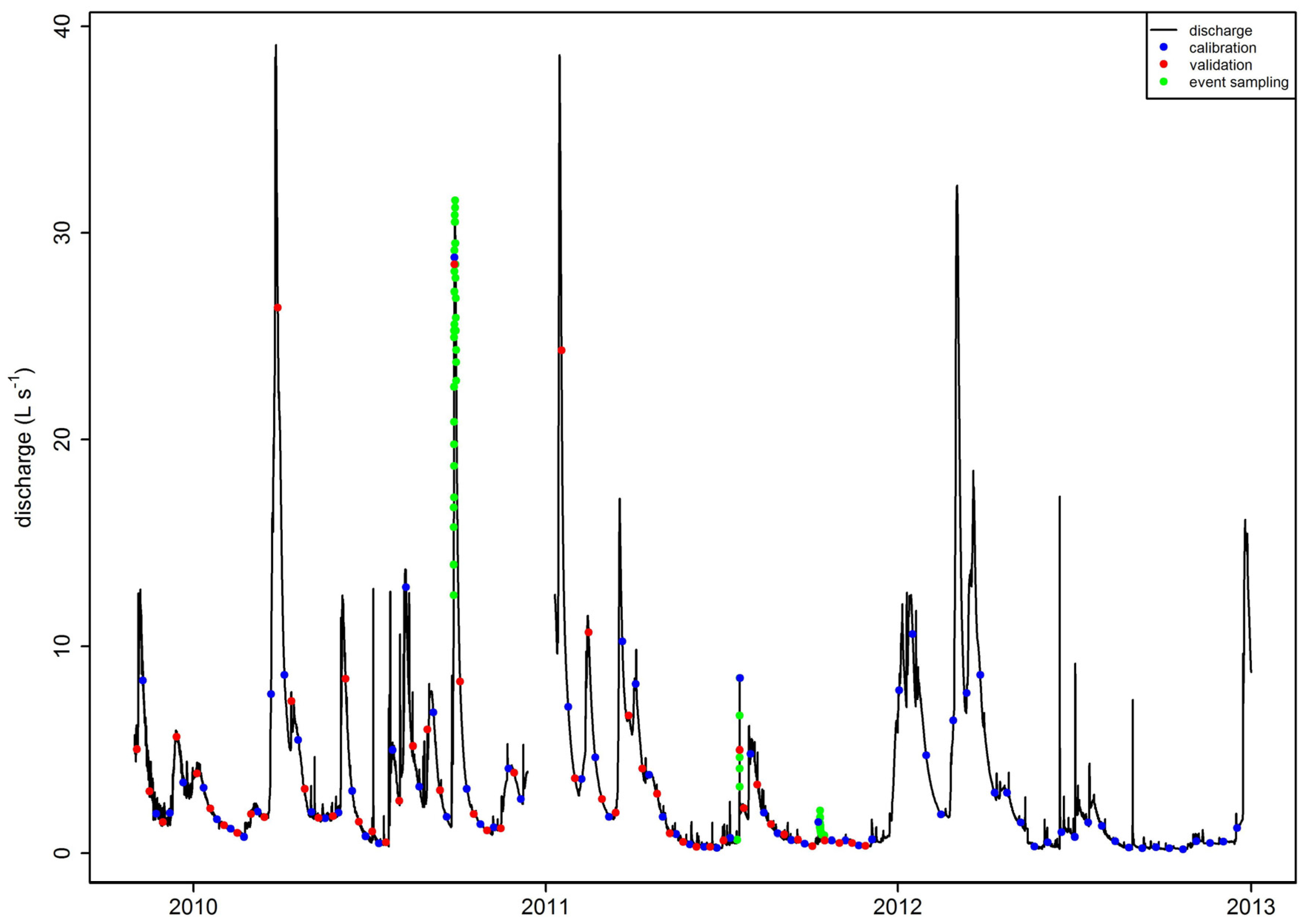
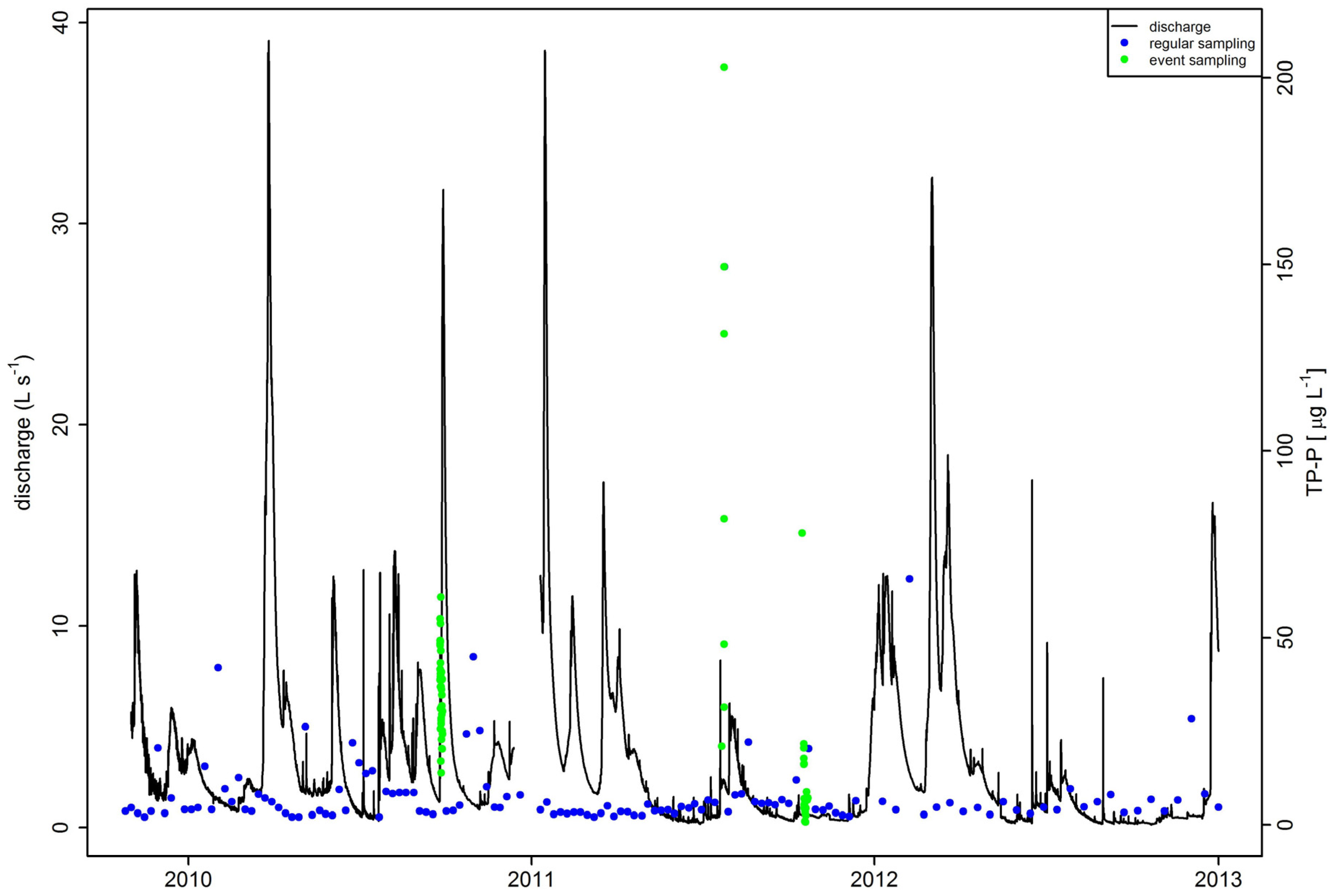
2.2. Water Sampling and Chemical Analysis

At the outlet of the studied watershed, a V-shaped weir was installed, and the water level was recorded at 5-minute intervals using an ISCO™ 3220/4220 Submerged Probe Flow Meter. Discharge was then calculated using the V-weir specific rating curve at each recorded time step [19]. From September 2009 to December 2011, instantaneous water samples were taken at weekly intervals, and in 2012 the water sampling was conducted at bi-weekly intervals (Figure 1).
During the course of the measurements, three events (Event 1 = September 2010; Event 2= July 2011; Event 3 = October 2011) were sampled using an automatic ISCO™ 3700 Portable Sampler. The frequency of sampling during the event was controlled by discharge. The event sampling began when a threshold water level in the stream was exceeded, and ceased when the level dropped back below the threshold (Figure 1). The collected samples (both fixed-schedule and event-based) were kept at 4 °C during transportation until analysis. All samples were analyzed for electric conductivity, pH, and total phosphorus (TP-P) according to DIN EN ISO 6878 protocol (DIN—German Institute for Standardization, 2004). Immediately after receiving the samples in the laboratory, sulfuric acid was added to the unfiltered samples to prevent changes in TP-P concentrations. The unfiltered sample was digested with persulfate to convert TP-P to Ortho-P which was afterwards measured photometrically as molybdenum blue complex (wavelength of 880 nm).

2.3. Load Calculations

Using the measured concentrations of TP-P and the measured discharges, fluxes of TP-P were then calculated. To assess the effect of the respective method, the P fluxes were calculated using several different load estimation methods (see Table 1). The measured time series of discharge was aggregated to hourly averages. With all methods, the fluxes were calculated for meteorological seasons: winter (December to February), spring (March to May), summer (June to August), and fall (September to November) for the time period between December 2009 to November 2012. This seasonal breakdown was made to allow for the assessment of contrasting moisture conditions and to reveal any potential effects on P flux dynamics.
Table 1 provides an overview of the applied load calculation methods used in this study. The discharge-weighted flux estimation method is the only interpolation method [15] used in this study. In this method, loads estimation was based on the measured discharge and solute concentration during the sampling, and the average discharge between the sampling times. All other applied methods are extrapolation methods, where a statistical relationship between the measured discharge and solute concentration is first established. Using this relationship, the solute concentration for the times without samples is estimated based on the measured discharge. The extrapolation methods differ in the method used to establish the discharge-solute relationship [9,20]. The interpolation models shown in Table 1 were applied using the R-package loadflex [20]. Here, the discharge-solute concentration relationship is established by connecting the measured solute concentration using different means of interpolation (e.g., rectangular, triangular, spline, distance-weighted, etc.) [20]. For the linear model, a linear regression is fitted with the log-discharge and log-solute concentration [20]. For the Loadest regression models (Table 1), non-linear regression functions between measured discharge and solute concentrations were established [22,23,24].
For the calculation of the Webb interpolation method, the entire data set from the fixed-schedule sampling was used. For all other methods (see Table 1), the data set obtained by the fixed-schedule sampling was split into “calibration” and “validation” sections (see also Figure 1). For the period from December 2009 to December 2011, weekly samples were available, while bi-weekly samples were available during 2012. The finest temporal resolution available for the entire data period was therefore bi-weekly, which was then used to establish the discharge-solute concentration relationships for all methods listed in Table 1, using the R-package loadflex [20]. After the establishment of the load calculation models, loadflex was used to predict the P fluxes for the time steps without TP-P measurements using the measured discharge as a predictor. The remaining data from the fixed-schedule samples was used to assess the quality of the predicted loads. From the predicted load time series, data points were extracted where data for validation was available.
In order to evaluate the quality of the predictions, the coefficient of determination (R²) and the mean absolute error (MAE, Equation (1)) for the predicted and observed data of the validation data set were calculated. Bennet et al. [25] proposed that R² should be combined with error statistics like Bias. The advantage of the MAE is that the error is expressed in the units of the fluxes and is not affected by cancellation, unlike Bias [25], which makes the interpretation easier.
M A E = 1 n i = 1 n | p i o i |
With oi the observed values and pi the predicted values at time step i.
To compare the differences in flux-export calculation between the fixed-schedule sampling data set and the extended data set containing the event data (fixed-schedule + events), the above described load calculation procedures were applied to two data sets. The first data set relied on the fixed-schedule sampling, as described above, and was split into a calibration and validation part for the extrapolation methods (Figure 1). The second data set consisted of the concentration measurements from the fixed-schedule sampling amended with the two sampling points of each sampled event, which were close to peak discharge (Figure 1). This data set was also split into calibration and validation periods, as described above. The inclusion of more data from the events was not possible, since the extrapolation methods require at least 6 to 7 days between the samples to avoid auto-correlation [20,22].
For comparison of the predicted export fluxes of TP-P for the extrapolation methods, the best three models for each data set (fixed-schedule and fixed-schedule + events) based on their R² and MAE during validation were selected. These two groups are henceforth referred to as LF-R (the three best extrapolation models based on the fixed-schedule data set) and LF-E (the three best extrapolation models based on the extended data set). These groups were compared to two export flux predictions from the Webb based interpolation method using the fixed-schedule sampling data set (Webb-R) and based on the extended data set (Webb-E).

3. Results and Discussion

3.1. Phosphorus Concentrations

Table 2 summarizes the measured discharge rates, as well as the measured TP-P concentrations during the fixed-schedule sampling for the study period. The highest maximum and mean discharge values were measured in winter and spring following the seasonal periods with wet soils, low transpiration, and snow melt. The TP-P concentrations ranged from 2.0 to 65.7 μg·L−1 across all seasons, with the highest maximum and mean values observed in the winter. The mean concentrations during winter, summer, and fall are within the same ranges (10.6, 7.8, and 9.3 μg·L−1), while the mean concentration during spring is significantly lower (4.6 μg·L−1). From Table 2 it also can be seen that the maximum sampled discharge is smaller than the maximum total discharge throughout the season. This indicates that the fixed-schedule sampling scheme did not capture many of the high-flow conditions.
Table 3 summarizes the measured discharge values and TP-P-concentrations during the storm event-based monitoring. Event 1 (September 2010) had the highest discharge (31.6 L·s−1), with TP-P concentrations ranging from 2.7 to 60.9 μg·L−1 during the event. The highest concentrations during a storm event was found during Event 2, with TP-P concentration ranging from 21 to 202 μg·L−1 and with discharge as high as 8.5 L·s−1.
Event 3 had the lowest measured discharge of the sampled storm events, with TP-P concentrations ranging from values below the detection limit up to 78 μg·L−1, with a mean concentration of 11.4 μg·L−1 for the whole event.
The results show that the dynamics of TP-P concentrations are highly variable, both over the course of seasons, during low flow periods, and during storm events (i.e., high-flow periods). As shown in Figure 2, the TP-P concentrations varied over several orders of magnitude, ranging from values below the detection limit to very high concentrations after heavy rainfall events. The highest concentrations were measured during events in summer and fall after long dry periods with little or no precipitation.
The increased concentration of TP-P during the summer and fall seasons indicates that during dry periods P accumulates in the soil, which then is flushed by precipitation water during rain events [6]. Recent studies have demonstrated that dry and rewetting cycles, which occur more often during summer and fall seasons, increase the export of P from the organic layers and upper mineral horizons [26]. In forest soils, mobilized P is typically transported via preferential flow pathways, such as root channels, stone surfaces, and at the interface between organic and mineral horizons laterally down slope to streams [8,27]. Lateral subsurface flow is frequently the dominant discharge generation process in small forested mountain catchments [28]. In the Eastern Ore Mountains, lateral subsurface flow is driven by the characteristics of periglacial cover beds over bedrock, which are prevalent in this area [29,30]. During dry periods with low soil moisture, the formation of near surface lateral flow is more frequent [29], which explains the rapid catchment response to storm events and the higher TP-P concentrations.
As can be seen from the results of the different sampling schemes (e.g., fixed-schedule and event-based, compared mean and max concentrations in Table 2 and Table 3), the highly dynamic changes in P concentrations were not fully captured by the fixed-schedule sampling at either the weekly or bi-weekly time scale. During the dry summer and fall seasons, where P exports from soils are driven primarily by the change of accumulation and flushing (as discussed above), P concentrations in streams in forested catchments can change drastically within a day, or even at sub-daily time scales. A weekly or bi-weekly sampling scheme is therefore not able to entirely capture those changes, and does not provide an adequate enough representation of P dynamics necessary for process understanding [13]. This information gap will therefore increase process uncertainty [11], which will propagate into the estimation of P export fluxes [10,11,18].

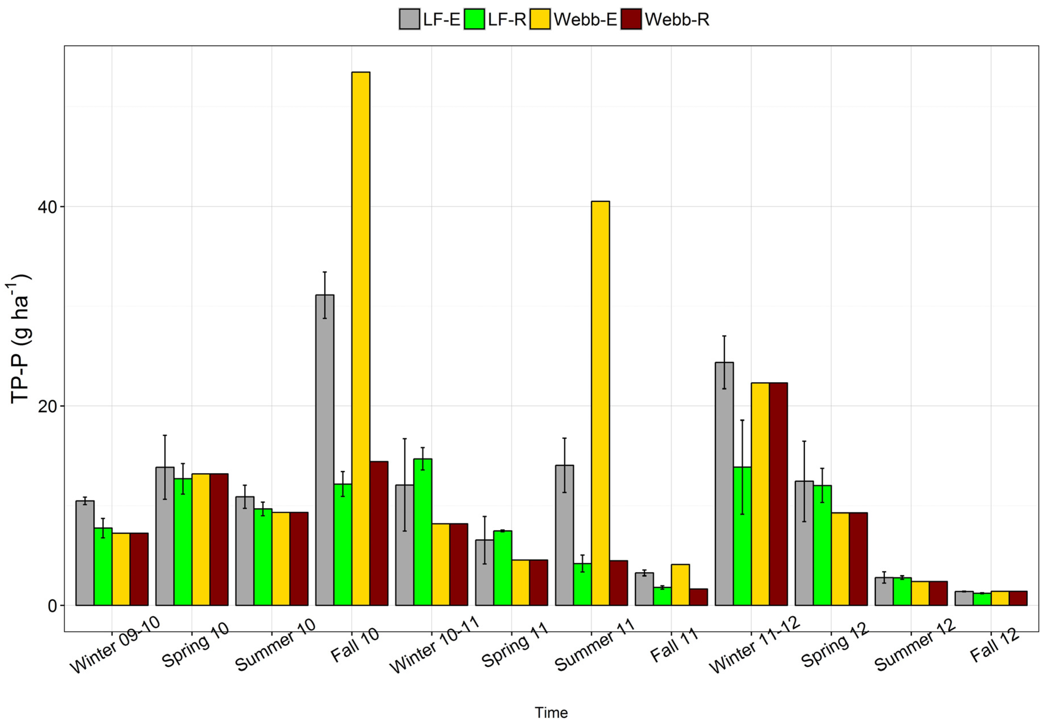
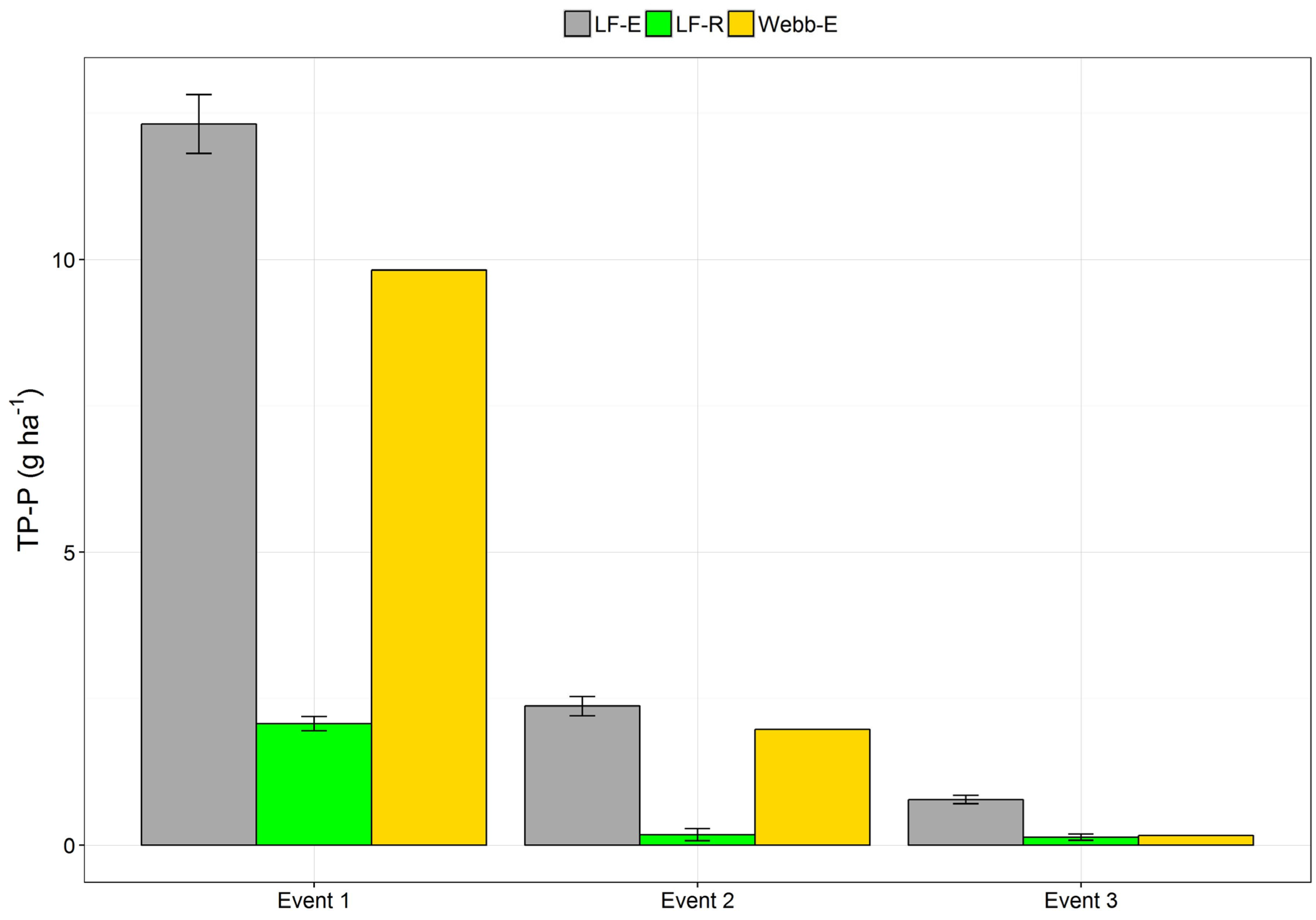
3.2. Phosphorus Fluxes

Table 4 provides a summary of the evaluation criteria for each of the applied loadflex models. All criteria were calculated during the independent validation time period (see Figure 1). A wide range of values for the coefficient of determination (R²) were observed from both the fixed-schedule and extended sample data sets. Values for the prediction models ranged from 0.41 to 0.67 for the fixed-schedule sampling data set, and from 0.37 to 0.97 for the extended sampling data set. It is clear that for both data sets, only a limited number of models established a good relationship between the predicted and the observed TP-P loads. The MAE measures the difference between predicted and observed TP-P loads. MAE values close to zero indicate a good agreement between the prediction and observations. All prediction models based on the two data sets had small values for MAE, with values ranging from 0.05 to 0.27 g·ha−1·d−1 over the 2-year validation period. The inclusion of data from the event sampling (extended data set) led to an improvement in the relationship between observed and predicted TP-P loads, and only to small increases in the MAE. Therefore, it can be concluded that the prediction quality was increased with the inclusion of the event-based data. For analysis of the TP-P flux export rates, the models Trian. I., Reg. Mod. 4, and Reg. Mod. 7 will be referred to as LF-R (based on the fixed-schedule sampling data set) and the models Lin. I., Trian. I., and Dist. Weigh. I. will be referred to as LF-E (based on the extended data set). These models were chosen because they showed the best fit to the independent validation data set. The other models were not considered in the analysis of the export fluxes.
Table 5 provides the predicted annual TP-P fluxes for the different groups of load estimation techniques (LF-R, LF-E, Webb-R, and Webb-E). All methods show a similar pattern, with higher TP-P exports in 2010 and lower in 2011 and 2012. Three single storm events were monitored in 2010 and 2011, during which Webb-E estimated the highest TP-P export, followed by LF-E, Webb-R, and LF-R. No storm events were recorded in 2012, during which LF-E predicted slightly higher export rates than the other three groups. The amount of predicted TP-P exports followed the observed annual rainfall, with 2010 having the highest rainfall and 2011 the lowest.
The TP-P fluxes follow the variation of discharge and concentration over the course of the seasons, as can be seen from Figure 3 (flux rates), Figure 2 (concentration and discharge), and Table 2. In winter 2009/10, higher concentrations of TP-P were measured, but lower discharge was recorded (see Table 2), which results in fluxes between 7 to 10 g·ha−1 across all methods. In winter 2010/11, higher discharge values and lower TP-P concentrations resulted in slightly higher export rates when compared to the preceding winter season, with values ranging between 8 and 15 g·ha−1. The highest TP-P concentrations were measured in the winter of 2011/12, with average discharge amounts ranging from 14 to 25 g·ha−1. For spring 2010 and 2012, flux rates ranged from 9 to 13 g·ha−1 across all methods. Both seasons were comparable in terms of discharge rates, with maximum flow rates of 39.1 and 32.2 L·s−1, and average discharge of 5.6 and 5.7 L·s−1 for spring 2010 and spring 2012, respectively. The only significant difference was the higher rainfall of 284 mm in spring 2010, compared to 181 in spring 2012. It can be assumed that much of the discharge in spring 2012 was induced by snowmelt, since the preceding winter seasons had average discharges with high precipitation of 531 mm, of which a significant part was in the form of snow. The TP-P fluxes in spring 2011 were almost 50% lower compared to the other spring season, with rates ranging from 4.5 to 7.5 g·ha−1. The maximum and average discharge was also lower in spring 2011 compared to the other spring seasons, with values of 17.2 and 3.5 L·s−1. For summer 2010, all methods predicted TP-P fluxes around 10 g·ha−1, with relatively high mean and maximum TP-P concentrations, and medium average discharge and higher maximum discharge. For the summer 2011, the estimated TP-P flux rates across the applied methods differed significantly, with loads ranging from 4 to 40 g·ha−1. For this season, a single storm event-based sample was available (see Table 3, Event 2), where high TP-P concentrations were observed.
The calculation groups based on the fixed-schedule sampling (LF-R and Webb-R) gave equal flux rates of around 4 g·ha−1, whereas the methods based on the extended data differed significantly, with a value of 24 g·ha−1 for LF-E and 40 g·ha−1 for Webb-E. For summer 2012, all methods predicted low flux rates of 2 to 3 g·ha−1, due to low discharge and low TP-P concentrations during a long dry period. As in summer 2012, for fall 2010, information of a single storm event was available, which resulted in a wide range of estimated TP-P fluxes across the applied methods (ranging from 12 to 53 g·ha−1). For this season as well, the flux calculation based on the fixed-schedule sampling provided comparable rates, with 12 and 14 g·ha−1 for LF-R and Webb-R, respectively. The calculations made using the storm event data resulted in much higher values, with 31 g·ha−1 for LF-E and 53 g·ha−1 for Webb-E. Despite the inclusion of a single storm event for fall 2011, the calculated exports across all applied methods were relatively low, with flux rates ranging from 1.7 to 4 g·ha−1. For this season, the flux estimation for LF-R and Webb-R were in the same range (approx. 1.7 g·ha−1) and the estimates for LF-E and Webb-E were slightly higher (3.3 to 4.1 g·ha−1). The monitored event was relatively short, with low discharge and medium TP-P concentrations (Table 2). For fall 2012, all methods estimated low export rates of around 1.3 g·ha−1, due to a dry period with low discharge and medium TP-P concentrations.
The three monitored single storm events differed in magnitude of discharge and measured TP-P concentrations, as well as in duration of the storm and preceding conditions (e.g., length of dry periods; see also Table 3 and Figure 2). The different conditions resulted in different export rates of P during those events (Figure 4). The calculated export rates vary also across the applied method and the underlying data. For Event 1 in fall 2010, export rates varied from 2.1 to 12.3 g·ha−1 between the different methods. The lowest flux estimation was given by LF-R, whereas LF-E and Webb-E predicted much higher loads (12.3 and 9.8 g·ha−1, respectively). According to the LF-E method, this single event produced 40% of the total TP-P exports in fall 2010. For LF-R and Webb-E, the shares were 17% and 18%, respectively. For the total flux in year 2010, the portions were 19%, 5%, and 12% for LF-E, LF-R, and Webb-E. During the second monitored event in summer 2011, 0.2 to 2.4 g·ha−1 TP-P were exported. As for Event 1, the LF-R method predicted much lower flux rates than LF-E and Webb-E (2.4 and 2.0 g·ha−1, respectively). This event was characterized by high P concentrations but low discharge and a short duration. This event occurred after a long dry period with low precipitation and discharge in the preceding weeks, so P could have accumulated in the organic and mineral layer of the soil, which then flushed out during the event. The share for the total TP-P flux in summer 2011 was 17%, 4%, and 5% for LF-E, LF-R, and Webb-E. The event contributed to 7% of the total TP-P flux in year 2011 for LF-E, 1% for LF-R, and 4% for Webb-E. The third monitored event occurred in fall 2011 after a long dry period with low-flow conditions. For this event, LF-E calculated export rates of 0.8 g·ha−1, whereas LF-R and Webb-E calculated 0.1 and 0.2 g·ha−1. This event contributed to 24% of the annual total TP-P flux for LF-E, 6% for LF-R, and 5% for Webb-E. The shares for the total flux in year 2011 were 2%, 0.4%, and 0.4% for LF-E, LF-R, and Webb-E, respectively.
The predicted annual export fluxes of TP-P ranged from 18.5 to 83.2 g·ha−1 depending on the year and selected load calculation method. These values are in the same range as previous studies for watersheds in other regions of Europe [4,5,16], but lower than findings for catchments dominated by monsoonal influence [10,18]. Further, the seasonality of the export is driven by high discharge due either to snow melt in the winter/spring or due to rainfall events following a dry period where P could accumulate in the soil. It was observed that the event-based export of P can contribute up to 40% to the seasonal and 19% to the annual export fluxes, which highlights the importance of monitoring stormflow events for flux estimation and process understanding. These results support the findings of numerous studies [9,11,18,31] which have found that time discrete sampling schemes at the monthly or bi-weekly time scale are unable to capture short-term changes in solute concentrations, and therefore can lead to a bias in load calculations. Ide et al. [18] suggested that a certain number of monitored stormflow events are necessary to quantify export fluxes with low bias. The results of our study also suggest that the differences in the flux estimates between the selected methods are smaller than the differences due to the sampling scheme (i.e., see the error bars in Figure 3 and Figure 4). Finally, we can assume that for the quantification of P export fluxes from forests, an adequate monitoring scheme of stream exports is necessary to be able to capture short-term changes in P concentrations.

4. Conclusions

The TP-P concentrations observed in stream-water varied significantly over the course of the year, with particularly high concentrations found during single storm events where discharge significantly rose compared to pre-event conditions. During the high flow periods, which were induced by snow melt at the end of the winter season or the beginning of the spring season, the TP-P concentration was decreased. During the storm events, TP-P was likely exported from the soil to the riverine system via near surface lateral flow through preferential flow paths, or at the interface between the organic and mineral soil layers. Based on the event sampling and the method used for flux calculation, up to 12 g·ha−1 of TP-P can be exported during a single storm event, which can contribute up to 40% to seasonal fluxes and up to 19% to annual fluxes. The magnitude of the exports depends on the intensity of rainfall, reaction of the catchment to the event, and the pre-event conditions, such as the length of the preceding dry period. Depending on the method used for estimating fluxes, and on the data set, annual export rates ranged from 19 up to 83 g·ha−1·a−1. In most cases the Webb based flux estimations were lower than the loadflex-based predictions in the winter and spring seasons, but most often the fluxes were in the same range, with values from 3 to 9 g·ha−1. In the three seasons where events were monitored, the major difference was between the estimations relying only on the data of the fixed-schedule sampling and the estimations where additional information was available from the event sampling. The predictions depending on the fixed-schedule sampling data set were in the same range for all three seasons. The prediction methods (LF + Webb) based on the extended information showed higher fluxes, but also differed significantly from each other, with Webb calculating the highest fluxes. We can assume that predictions of TP-P export rates based on a sampling strategy which does not consider short-term changes due to factors such as storms will substantially underestimate P exports.

Acknowledgments

This study is based on results of the project REGKLAM (Development and Testing of an Integrated Regional Climate Change Adaptation Programme for the Model Region of Dresden), project no. 01LR0802B financed by the German Federal Ministry for Education and Research (BMBF). The authors thank Ruth Rüger, Ina Klemm, Claudia Thiere, and Thomas Klinger for the laboratory analysis and Norbert Prange for his support during the field campaigns. Special thanks go to Daniel Hawtree for the language editing of the manuscript.

Author Contributions

S.J. did the data analysis; R.B. did the field work; all authors wrote the manuscript.

Conflicts of Interest

The authors declare no conflict of interest.

References

  1. Lang, F.; Bauhus, J.; Frossard, E.; George, E.; Kaiser, K.; Kaupenjohann, M.; Krüger, J.; Matzner, E.; Polle, A.; Prietzel, J.; et al. Phosphorus in forest ecosystems: New insights from an ecosystem nutrition perspective. J. Plant Nutr. Soil Sci. 2016, 179, 129–135. [Google Scholar] [CrossRef]
  2. Walker, T.W.; Syers, J.K. The fate of phosphorus during pedogenesis. Geoderma 1976, 15, 1–19. [Google Scholar] [CrossRef]
  3. Haygarth, P.M.; Hepworth, L.; Jarvis, S.C. Forms of phosphorus transfer in hydrological pathways from soil under grazed grassland. Eur. J. Soil Sci. 1998, 49, 65–72. [Google Scholar] [CrossRef]
  4. Vuorenmaa, J.; Rekolainen, S.; Lepistö, A.; Kenttämies, K.; Kauppila, P. Losses of Nitrogen and Phosphorus from Agricultural and Forest Areas in Finland during the 1980s and 1990s. Environ. Monit. Assess. 2002, 76, 213–248. [Google Scholar] [CrossRef] [PubMed]
  5. Verheyen, D.; Gaelen, N.V.; Ronchi, B.; Batelaan, O.; Struyf, E.; Govers, G.; Merckx, R.; Diels, J. Dissolved phosphorus transport from soil to surface water in catchments with different land use. AMBIO 2015, 44, 228–240. [Google Scholar] [CrossRef] [PubMed]
  6. Bol, R.; Julich, D.; Brödlin, D.; Siemens, J.; Kaiser, K.; Dippold, M.A.; Spielvogel, S.; Zilla, T.; Mewes, D.; von Blanckenburg, F.; et al. Dissolved and colloidal phosphorus fluxes in forest ecosystems—an almost blind spot in ecosystem research. J. Plant Nutr. Soil Sci. 2016, 179, 425–438. [Google Scholar] [CrossRef]
  7. van der Heijden, G.; Legout, A.; Pollier, B.; Bréchet, C.; Ranger, J.; Dambrine, E. Tracing and modeling preferential flow in a forest soil—Potential impact on nutrient leaching. Geoderma 2013, 195–196, 12–22. [Google Scholar] [CrossRef]
  8. Julich, D.; Julich, S.; Feger, K.-H. Phosphorus in Preferential Flow Pathways of Forest Soils in Germany. Forests 2016, 8, 19. [Google Scholar] [CrossRef]
  9. Kerr, J.G.; Eimers, M.C.; Yao, H. Estimating stream solute loads from fixed frequency sampling regimes: The importance of considering multiple solutes and seasonal fluxes in the design of long-term stream monitoring networks. Hydrol. Process. 2016, 30, 1521–1535. [Google Scholar] [CrossRef]
  10. Yanai, R.D.; Tokuchi, N.; Campbell, J.L.; Green, M.B.; Matsuzaki, E.; Laseter, S.N.; Brown, C.L.; Bailey, A.S.; Lyons, P.; Levine, C.R.; et al. Sources of uncertainty in estimating stream solute export from headwater catchments at three sites. Hydrol. Process. 2015, 29, 1793–1805. [Google Scholar] [CrossRef]
  11. Harmel, R.D.; Cooper, R.J.; Slade, R.M.; Haney, R.L.; Arnold, J.G. Cumulative uncertainty in measured streamflow and water quality data for small watersheds. Trans. ASABE 2006, 49, 689–701. [Google Scholar] [CrossRef]
  12. Horowitz, A.J. A Review of Selected Inorganic Surface Water Quality-Monitoring Practices: Are We Really Measuring What We Think, and If So, Are We Doing It Right? Environ. Sci. Technol. 2013, 47, 2471–2486. [Google Scholar] [CrossRef] [PubMed]
  13. Kirchner, J.W.; Feng, X.; Neal, C.; Robson, A.J. The fine structure of water-quality dynamics: The (high-frequency) wave of the future. Hydrol. Process. 2004, 18, 1353–1359. [Google Scholar] [CrossRef]
  14. Ullrich, A.; Volk, M. Influence of different nitrate–N monitoring strategies on load estimation as a base for model calibration and evaluation. Environ. Monit. Assess. 2010, 171, 513–527. [Google Scholar] [CrossRef] [PubMed]
  15. Webb, B.W.; Phillips, J.M.; Walling, D.E.; Littlewood, I.G.; Watts, C.D.; Leeks, G.J.L. Load estimation methodologies for British rivers and their relevance to the LOIS RACS(R) programme. Sci. Total Environ. 1997, 194–195, 379–389. [Google Scholar] [CrossRef]
  16. Palviainen, M.; Finér, L.; Laurén, A.; Launiainen, S.; Piirainen, S.; Mattsson, T.; Starr, M. Nitrogen, Phosphorus, Carbon, and Suspended Solids Loads from Forest Clear-Cutting and Site Preparation: Long-Term Paired Catchment Studies from Eastern Finland. AMBIO 2013, 43, 218–233. [Google Scholar] [CrossRef] [PubMed]
  17. Kunimatsu, T.; Hamabata, E.; Sudo, M.; Hida, Y. Comparison of nutrient budgets betwen three forested mountain watersheds on granite bedrock. Water Sci. Technol. 2001, 44, 129–140. [Google Scholar] [PubMed]
  18. Ide, J.; Chiwa, M.; Higashi, N.; Maruno, R.; Mori, Y.; Otsuki, K. Determining storm sampling requirements for improving precision of annual load estimates of nutrients from a small forested watershed. Environ. Monit. Assess. 2012, 184, 4747–4762. [Google Scholar] [CrossRef] [PubMed]
  19. Benning, R.; Schua, K.; Schwärzel, K.; Feger, K.H. Fluxes of Nitrogen, Phosphorus, and Dissolved Organic Carbon in the inflow of the Lehnmühle reservoir (Saxony) as compared to streams draining three main land-use types in the catchment. Adv. Geosci. 2012, 32, 1–7. [Google Scholar] [CrossRef]
  20. Appling, A.P.; Leon, M.C.; McDowell, W.H. Reducing bias and quantifying uncertainty in watershed flux estimates: The R package loadflex. Ecosphere 2015, 6, 1–25. [Google Scholar] [CrossRef]
  21. Verma, S.; Markus, M.; Cooke, R.A. Development of error correction techniques for nitrate-N load estimation methods. J. Hydrol. 2012, 432–433, 12–25. [Google Scholar] [CrossRef]
  22. Lorenz, D.; Runkel, R. Rloadest: River Load Estimation; U.S. Geological Survey: Mounds View, MN, USA, 2015.
  23. Runkel, R. Revisions to LOADEST; U.S. Geological Survey: Reston, VA, USA, 2013.
  24. Runkel, R.; Crawford, C.; Cohn, T. Load Estimator (LOADEST): A FORTRAN Program for Estimating Constituent Loads in Streams and Rivers; Techniques and Methods Book 4; U.S. Geological Survey: Reston, VA, USA, 2004.
  25. Bennett, N.D.; Croke, B.F.W.; Guariso, G.; Guillaume, J.H.A.; Hamilton, S.H.; Jakeman, A.J.; Marsili-Libelli, S.; Newham, L.T.H.; Norton, J.P.; Perrin, C.; et al. Characterising performance of environmental models. Environ. Model. Softw. 2013, 40, 1–20. [Google Scholar] [CrossRef]
  26. Dinh, M.-V.; Schramm, T.; Spohn, M.; Matzner, E. Drying–rewetting cycles release phosphorus from forest soils. J. Plant Nutr. Soil Sci. 2016, 179, 670–678. [Google Scholar] [CrossRef]
  27. Julich, D.; Julich, S.; Feger, K.-H. Phosphorus fractions in preferential flow pathways and soil matrix in hillslope soils in the Thuringian Forest (Central Germany). J. Plant Nutr. Soil Sci. 2017, 180, 407–417. [Google Scholar] [CrossRef]
  28. Barthold, F.K.; Woods, R.A. Stormflow generation: A meta-analysis of field evidence from small, forested catchments. Water Resour. Res. 2015, 51, 3730–3753. [Google Scholar] [CrossRef]
  29. Heller, K.; Kleber, A. Hillslope runoff generation influenced by layered subsurface in a headwater catchment in Ore Mountains, Germany. Environ. Earth Sci. 2016, 75, 943. [Google Scholar] [CrossRef]
  30. Hübner, R.; Heller, K.; Günther, T.; Kleber, A. Monitoring hillslope moisture dynamics with surface ERT for enhancing spatial significance of hydrometric point measurements. Hydrol. Earth Syst. Sci. 2015, 19, 225–240. [Google Scholar] [CrossRef]
  31. Worrall, F.; Howden, N.J.K.; Burt, T.P. Assessment of sample frequency bias and precision in fluvial flux calculations—An improved low bias estimation method. J. Hydrol. 2013, 503, 101–110. [Google Scholar] [CrossRef]
Figure 1. Time series of measured discharge with sampling points; blue dots: data used to establish the respective load calculation equations; red dots: data used only for validation; green dots: sampling during storm events.
Forests 08 00206 g001
Figure 2. Time series of measured discharge (black line) and TP-P concentration for the fixed-schedule sampling (blue dots) and during the event sampling (green dots).
Forests 08 00206 g002
Figure 3. Predicted seasonal TP-P export fluxes for the different load calculation method groups; the error bars indicate the differences between the three best load calculation models based on the validation. For Webb-E and Webb-R, no validation was possible (due to the method).
Forests 08 00206 g003
Figure 4. Predicted TP-P export fluxes for three monitored events for the different groups of load calculation methods; the error bars indicate the differences between the three best load calculation models based on the validation. For Webb-E, no validation was possible due to the method.
Forests 08 00206 g004
Table 1. Overview of the applied flux calculation methods. For the detailed calculation procedures, refer to the indicated references.
MethodAbbreviationReference
Discharge-weighted Flux estimationWebbMethod E in [15]
Linear InterpolationLin. I.[20]
Triangular InterpolationTriang. I.[20,21]
Rectangular InterpolationRect. I.[20,21]
Spline InterpolationSpl. I.[20]
Smooth Spline InterpolationSm. Spl. I.[20]
Distance Weighted InterpolationDist. Weigh I.[20]
Linear ModelLin. Mod.[20]
Loadest Regression Model 1Reg. Mod. 1[22,23,24]
Loadest Regression Model 2Reg. Mod. 2[22,23,24]
Loadest Regression Model 3Reg. Mod. 3[22,23,24]
Loadest Regression Model 4Reg. Mod. 4[22,23,24]
Loadest Regression Model 5Reg. Mod. 5[22,23,24]
Loadest Regression Model 6Reg. Mod. 6[22,23,24]
Loadest Regression Model 7Reg. Mod. 7[22,23,24]
Loadest Regression Model 8Reg. Mod. 8[22,23,24]
Loadest Regression Model 9Reg. Mod. 9[22,23,24]
Table 2. Overview of discharge during the whole period (Tot. Discharge), the sampled discharge (Samp. Discharge), and total phosphorus (TP-P) concentrations during the fixed-schedule sampling for the different seasons; with Min = Minima, Max = Maxima, Mn. = Mean, Md. = Median.
SeasonTot. Discharge (L·s−1)Samp. Discharge (L·s−1)TP-P (µg·L−1)
MinMaxMn.Md.MinMaxMn.Md.MinMaxMn.Md.
Winter 09–100.86.02.42.00.85.62.41.93.042.010.96.0
Spring 101.439.15.62.21.726.45.22.02.026.26.33.9
Summer 100.313.83.62.70.512.93.93.02.021.89.78.5
Fall 100.931.74.12.51.19.53.63.02.744.912.04.6
Winter 10–112.438.67.24.52.624.37.44.12.58.44.63.5
Spring 110.417.23.52.30.410.23.42.02.05.43.33.4
Summer 110.28.31.40.70.34.81.40.73.322.08.05.8
Fall 110.31.60.60.60.30.90.60.62.221.07.45.2
Winter 11–120.312.64.43.00.510.64.23.32.665.716.45.3
Spring 120.232.35.73.10.38.64.02.92.66.04.34.1
Summer 120.217.31.10.90.31.50.90.82.99.55.64.7
Fall 120.11.10.40.30.20.60.30.33.128.28.65.0
Table 3. Discharge, TP-P concentrations during the monitored events; with Min = Minima, Max = Maxima, Mn. = Mean, Md. = Median sampling schemes, b.d. = below detection limit.
EventDischarge (L·s−1)TP-P (µg·L−1)
MinMaxMn.Md.MinMaxMn.Md.
Event 112.531.625.826.42.760.934.336.8
Event 20.68.54.74.621.0202.895.181.9
Event 30.92.11.11.0b.d.78.011.46.5
Table 4. Overview of evaluation criteria for the load calculation methods used for the fixed-schedule data set (R) and the extended data set (E). Abbreviations of the methods are explained in Table 1; MAE in (g·ha−1·d−1); numbers in bold mark the models selected for further analysis (LF-R and LF-E).
MethodMAE
TP-PTP-P
RERE
Lin. I.0.440.960.050.12
Triang. I.0.620.970.060.14
Rect. I.0.410.910.060.15
Spl. I.0.460.940.050.13
Sm. Spl. I.0.610.360.060.27
Dist. Weigh I.0.500.970.050.12
Lin. Mod.0.610.370.050.26
Reg. Mod. 10.600.370.050.26
Reg. Mod. 20.550.370.060.26
Reg. Mod. 30.600.360.050.26
Reg. Mod. 40.670.600.050.24
Reg. Mod. 50.560.370.060.26
Reg. Mod. 60.560.600.050.24
Reg. Mod. 70.660.600.050.24
Reg. Mod. 80.570.590.060.24
Reg. Mod. 90.570.600.060.24
Table 5. Predicted annual TP-P loads (g·ha−1) by the different groups of export flux calculation methods. Mn. = Mean, Std.Dev. = Standard Deviation within the three selected extrapolation models for each group, n.a.= not applicable.
YearLF-RLF-EWebb-RWebb-E
Mn.Std.Dev.Mn.Std.Dev.Mn.Std.Dev.Mn.Std.Dev.
201042.31.166.31.844.2n.a.83.2n.a.
201128.20.635.92.518.9n.a.57.3n.a.
201229.91.741.01.835.4n.a.35.4n.a.

