
Fire Behavior Simulation from Global Fuel and Climatic Information


Environmental Remote Sensing Research Group, University of Alcala, Calle Colegios 2, 28801 Alcalá de Henares, Spain
*
Author to whom correspondence should be addressed.
Forests 2017, 8(6), 179; https://doi.org/10.3390/f8060179
Submission received: 13 March 2017
/
Revised: 11 May 2017
/
Accepted: 12 May 2017
/
Published: 24 May 2017
Abstract
:Large-scale fire danger assessment has become increasingly relevant in the past few years, and is usually based on weather information. Still, fuel characteristics also play an important role in fire behavior. This study presents a fire behavior simulation based on a global fuelbed dataset and climatic and topographic information. The simulation was executed using the Fuel Characteristic Classification System (FCCS). The climatic information covered the period 1980–2010, and daily weather parameters were used to calculate the mean monthly fuel moisture content (FMC) and wind speed for the early afternoon period. Also, as the most severe fires occur with extreme environmental conditions, a worst-case scenario was created from the 30 days of each month with the lowest FMC values for the 1980–2010 period. The FMC and wind speed information was grouped into classes, and FCCS was used to simulate the reaction intensity, rate of spread and flame length of the fuelbeds for the average and worst-case monthly conditions. Outputs of the simulations were mapped at global scale, showing the variations in surface fire behavior throughout the year, both due to climatic conditions and fuel characteristics. The surface fire behavior parameters identified the fuels and environmental conditions that produced more severe fire events, as well as those regions where high fire danger only occurs in extreme climatic conditions. The most severe fire events were found in grasslands and shrublands in tropical dry biomes, and corresponding with the worst-case scenario environmental conditions. Also, the results showed the importance of including detailed fuel information into fire danger assessment systems, as the same weather and topographic conditions may have different danger rates, depending on fuel characteristics.
1. Introduction
Wildfires occur due to a combination of available fuels, sources of ignition, and environmental conditions (mostly weather but also topography), that allow fire to be sustained and spread. Within these variables, weather is the most fluctuating one and is one of the largest drivers of fire behavior. For this reason, the relations of weather variables and fire occurrence have been widely studied [1,2,3,4]. Furthermore, several studies have analyzed the role of climate change in fire regime trends [3,5,6,7], emphasizing the need to better understand fire–weather relations.
Most fire behavior modeling systems consider weather variables to estimate critical parameters, such as rate of spread, flame length or the energy released [1]. The most common variables for those simulations are fuel moisture (estimated as a function of temperature, humidity and precipitation), wind speed, and terrain conditions (such as slope or aspect). Examples of widely-used fire behavior models are BehavePlus [8], the National Fire Danger Rating System [9], the Canadian Forest Fire Behavior Prediction System [10], and the Fuel Characteristic Classification System [11]. These systems were developed for regional or national territories, where fuel characteristics information is available, and were calibrated for the specific conditions of those areas [12]. When using them for estimating fire behavior potentials in other regions or countries, the existing fuel models might not represent properly the fuel characteristics in those areas [13,14,15]. This is particularly relevant for continental and global fire danger assessment [16,17].
Most existing national or continental fire danger systems rely mainly on weather information, using in many cases the Fire Weather Index (FWI) [18] developed as part of the Canadian Forest Fire Danger Rating System (CFFDRS) [10] or adaptations of it. Some examples of weather-based fire danger systems are the European Forest Fire Information System [19], Thailand’s Fine-Resolution Forecast Products of Fire Danger Rating System [20], and the Australian National Fire Danger Rating System [21,22]. There is also interest in studying fire danger at a global scale, as shown by the Global Early Warning System for Wildland Fires [16,23,24] and the Global Wildfire Information System [25,26].
Diverse fuels present very different responses to the same environmental conditions, as they may have different burnable biomass, size distribution (smaller fuels have more surface in contact with the heat), or flammable compounds. In addition, different fuels can also affect their microclimate under the same weather conditions [27], making them more or less fire-prone in a specific environmental situation. Even the same fuel structure with the same weather conditions can have diverse fire dynamics depending on vegetation species, as has been shown for boreal forests in Rogers et al. [28] and de Groot et al. [29]. Consequently, if fire risk assessment is based only on meteorological data, the systems employed need to be parameterized to cope with the absence of actual fuel information.
For these reasons, generating fuel maps with their associated characteristics is becoming increasingly relevant. Driven by this interest, we developed a global fuel map that includes the necessary parameters to obtain fire behavior predictions [30]. This map used as target categories the fuelbed concept proposed by the Fuel Characteristic Classification System (FCCS) [11]. The fuel parameters included in our product showed reasonable similarities with external global databases, such as those estimating above-ground biomass [30,31,32,33,34]. In developing this global fuel map, we also tested the estimation of fire potentials for different continents [35,36]. However, in those cases we based those estimations on default environmental parameters proposed by FCCS, corresponding to dry weather conditions. The use of a defined set of environmental conditions allowed the comparison of the different fuelbeds based solely on their intrinsic characteristics, but they did not reflect the variations of weather conditions around the world, which influence fire behavior predictions.
The main goal of this analysis was to provide a first estimation of fire behavior parameters at global scale using both fuel characteristics and environmental information. We simulated surface fire behavior conditions based on the FCSS, using fuel, topographic and meteorological data. Fuel properties were derived from a global fuel type product that we previously generated [30]. Topographic information was computed from GTOPO30. Climatic data were extracted from the spatially-distributed outputs of the ERA-Interim Global Reanalysis [37]. Rate of spread, flame length and reaction intensity (RI) were computed. Average and worst-case conditions were considered.
2. Materials and Methods
FCCS was designed to represent the structural and geographic diversity in wildland fuels and combines the fuel properties into “fuelbeds”, which include the physical and chemical variables used to model fire behavior and fuel consumption, and predict emissions [38]. FCCS uses fuel characteristics (e.g., percentage cover, loading, depth) to calculate and report nine fire potentials, organized into three categories: surface fire behavior potential, crown fire potential and available fuel potential [39]. Based on input environmental variables, FCCS also predicts surface fire behavior parameters using a reformulation of the Rothermel [40] fire behavior model [41].
To calculate surface fire behavior values, FCCS requires the input of fuelbed parameters and a set of environmental variables that affect fire spread and intensity. From this data the system calculates three well-known fire behavior parameters of surface fires for each fuelbed, which are:
The environmental variables required by FCCS are the slope, the midflame wind speed, and the fuel moisture content (FMC) of the dead and live fine fuels, which were each grouped into a few classes. A summary of the methodology is included in Figure 1, and the different steps are described in the sections below.
2.1. Fuel Dataset
The distribution of fuels and their physical and chemical properties related to fire behavior were extracted from the Global Fuel Dataset developed by Pettinari and Chuvieco [30]. This dataset was developed from different spatial variables, both based on satellite Earth observation products and fuel databases, and is comprised by two products:
- A global fuelbed map (Figure 2), with a spatial resolution of 10 arc seconds (approx. 300 m at the Equator), based on land cover and biomes information, and
- A database that includes the parameters of each fuelbed that affect fire behavior and effects.
The fuelbed dataset has 274 fuelbeds, 60 of them divided in two or three sub-fuelbeds according to their percentage of canopy cover, for a total of 359 fuelbeds and sub-fuelbeds. Each fuelbed is identified by a number, where the thousands value corresponds to the biome, and the following three values identify the land cover type associated with each pixel. For example, fuelbed 11,061 is in the Tundra biome (biome 11) and associated with broadleaved deciduous forests (land cover 061). The fuelbeds are organized into 6 strata: canopy, shrub, herb, woody fuels, litter–lichen–moss and ground fuels. The fuelbed database includes a list of associated structural, physical and chemical parameters of each fuelbed that influence fire behavior and effects, such as percent cover, height, loading, vegetation species, etc. These parameters were computed from external products, such as the MODIS Vegetation Continuous Fields collection 5 [43,44] to account for canopy cover, the Simard et al. [45] canopy height map to characterize canopy height, and existing fuel databases either included in FCCS or in Natural Fuels Photo Series from Mexico [46] and Brazil [47] for the rest of the parameters. This dataset is available at [48].
2.2. Climatic Data Source
The climatic data used to calculate the FMC and wind speed were extracted from the European Centre for Medium-Range Weather Forecasts (ECMWF) [49]. We used the ERA-Interim Global Reanalysis [37] because it was the ECMWF product that included all the required climatic variables and for the highest number of daily observations. Other ECMWF products considered, such as ERA-Interim/Land [50] and ERA-20CM [51], did not include all the climatic variables required to obtain the wind speed and fuel moisture content. Likewise, the ERA-20C reanalysis [52] did not provide as many daily observations as the ERA-Interim product.
The data used in this research covers a 30-year period, from 1981 until 2010, and was rescaled from the original 0.75° grid to a 0.50° grid covering the whole globe directly at the ECMWF Data Server. ERA-Interim provides global daily forecast information for 8 hours UTC (time steps): 0, 3, 6, 9, 12, 15, 18 and 21 h. Since the lowest fuel moisture content usually occurs at early afternoon, the globe was divided in 8 strips of 45° longitude, each one including information of local solar time between 12 h (in the western part of the strip) and 15 h (in the eastern part of the strip). Table 1 shows the longitudinal strips and a description of the ERA-Interim data used in each one, while Figure 3 shows the geographical distribution of each strip. For example, the data of UTC 15:00 was used for the strip extending between 45° and 90°, and that information represents weather conditions at 12 h for longitude 45°, 13 h for longitude 60°, 14 h for longitude 75° and 15 h for longitude 90°. Table 2 summarizes the variables used for this study and their characteristics.
2.3. Slope
Percentage slope was calculated using the Global 30 Arc-Second Elevation (GTOPO30) product. This is a global digital elevation model (DEM) with a horizontal grid spacing of 30 arcsec (approximately 1 km at the Equator), developed by the United States Geological Survey (USGS)—EROS Data Center [53].
Three slope classes were established with the following criteria (see Figure 4), to represent gentle, moderate and steep slopes:
- Slope class (SP) 1: 0% slope assigned in FCCS (for slopes between 0 and 5%),
- Slope class (SP) 2: 30% slope assigned in FCCS (for slopes between 5 and 45%),
- Slope class (SP) 3: 70% slope assigned in FCCS (for slopes higher than 45%).
The Chukchi Peninsula in eastern Russia (longitudes between 180° W and 169° W) did not have information in the GTOPO30, and Slope class 2 was assigned to that region.
2.4. Fuel Moisture Content
The fuel moisture content includes the following fuel classes: 1 h, 10 h, 100 h, live herbaceous, live shrub, and live crown. These FMC data were grouped in Fuel Moisture Scenarios (FMSs) [12] to simplify the analysis. Four FMSs were selected to represent different moisture conditions, and their values are indicated in Table 3.
To assign the FMSs, the 10 h FMC was calculated using the climatic variables extracted from the ECMWF. The National Fire Danger Rating System (NFDRS) [9] was used to calculate the 10 h FMC. The weather variables needed for the calculation of fire behavior were temperature, relative humidity, state of weather code (SOW), and the existence or not of precipitation or snow. The SOW is an assessment of the sky conditions at the observing time, which in the case of NFDRS represent the intensity of the insolation. The Total Cloud Cover variable from ECMWF was used to calculate the SOW, and the values obtained are represented as:
- 0: clear sky, less than 10% cloud cover,
- 1: scattered clouds, between 10 and 50% cloud cover,
- 2: broken clouds, between 60 and 90% cloud cover, and
- 3: overcast, 100% cloud cover.
The equilibrium moisture content (EMC) is in the base of the 10 h FMC calculation, and is the moisture content (%) of a fuel particle allowed sufficient time to reach equilibrium with its environment. This value is dependent on temperature (T) and relative humidity (RH), which are in turn corrected according to the SOW. The 10 h FMC is calculated as a proportion of the EMC.
The equations are:
If RH < 10%:
If 10% ≤ RH ≥ 50%:
If RH ≥ 50%:
If fuels are dry:
If fuels are wet at observation time (due to rain or snow):
where RH is relative humidity (%), T is temperature (°F), SOW is the state of weather code, and EMC is expressed in %. For the correction values of the SOW, refer to Cohen and Deeming [9].
The fuels were considered to be wet if the accumulated precipitation in the previous 24 h was at least 0.01 m, or if the snow depth was at least 0.001 m of water equivalent. As there was no RH value for each of the 8 time steps, the relative humidity was calculated from temperature and dew point values, using the formula [54]:
where TD is the dew point.
Once the 10-h FMC was calculated, it was used to assign the corresponding FMS, as follows:
- D1L1: 10 h FMC < 5.5%
- D2L2: 5.5% ≤ 10 h FMC < 8.5%
- D3L3: 8.5% ≤ 10h FMC < 10.5%
- D4L4: 10 h FMC ≥ 10.5%
The daily values of FMS obtained from the 1980 to 2010 climatic data were averaged in a monthly basis, to obtain the mean FMS for each month in each 0.5° cell, as a proxy to the mean conditions that could be found in that region during that month of the year. However, since extreme weather conditions (low FMC and high wind speed) are generally associated with large and severe fire events, a “worst-case conditions scenario” was created by calculating the mean FMS of the 30 days with the lowest monthly FMC of the 1980–2010 period.
2.5. Wind Speed
The wind speed data were downloaded from the ECMWF Data Server as the instantaneous U (from west to east) and V (from south to north) wind component speed at 10 m for each time step, as there was no daily variable with the resultant wind speed. Those component values were used to calculate wind speed with the formula:
Then it was necessary to transform the 10 m wind speed into midflame wind speed, to be able to compute it in FCCS. The midflame wind speed is the average wind velocity that affects surface fire spread, and is usually referred to as the velocity of the wind taken at the mid-height of the flames [40]. To do that, a wind adjustment factor (WAF) was assigned, which is as a function of the existing vegetation (considering if the surface fuels were sheltered or unsheltered from the wind), the surface fuel depth and the wind profile. As the wind information had a coarse resolution (0.5°) and at that scale it is not possible to take into consideration a particular vegetation profile, an intermediate value between sheltered and unsheltered fuels was used, corresponding to 0.4 for 20-ft winds (see Table 5 of Andrews [55]). This value was converted to 10-m winds using a conversion factor of 1.15 [56], to obtain a final WAF of 0.348.
As in the case of the slope, the midflame wind speed was grouped in three classes, to account for the contribution of wind to fire spread:
- Wind Class (WC) 1: 0–1.0 m·s−1 (0–2.24 mph). Assigned to 1.0 mph in FCCS.
- Wind Class (WC) 2: 1.0–2.5 m·s−1 (2.24–5.59 mph). Assigned to 4 mph in FCCS.
- Wind Class (WC) 3: 2.5–5 m·s−1 (5.59–11.18 mph). Assigned to 7 mph in FCCS.
The daily values of midflame wind speed were calculated for the 1980–2010 data, and aggregated by month to obtain the mean midflame wind speed for each month in each 0.5° cell. The resulting value was then converted to wind class. To account for the worst-case scenario, the midflame wind speed corresponding to the 30 worst-FMC-days in each month was obtained, and the values were averaged and then converted to wind class for those worst-case (extreme) conditions.
2.6. Fire Behavior
The possible FMSs, wind classes and slope classes created 36 combinations of possible environmental scenarios (shown in Table 4). Each fuelbed from the Global Fuelbed Dataset was run in the FCCS version 3.03.203 module inside the Fuel and Fire Tools [57] in all the scenarios, to obtain all possible ROS, FL and RI values for each fuelbed.
To create the predicted fire behavior maps, each fuelbed pixel in the fuelbed map was assigned the fire behavior results corresponding to the environmental scenario of their location and month that was being evaluated, both for the mean and extreme conditions. As the fuelbed map has a resolution of 10 arcsec, the resulting fire behavior results also had that resolution. For the purpose of facilitating the final representations, they were converted to 0.5° cell maps using the mean values within each cell.
3. Results
3.1. Environmental Conditions
The results obtained for January and July of the FMS and the wind class, both for the mean and worst-case scenario during the study period, are shown in the following figures. The results for the remaining months are shown in the Supplementary Materials (Tables S1 and S2) to this article.
Figure 5a shows the mean FMS conditions for January, where most of the world had a humid moisture scenario (D4L4), with the exception of the desertic regions. This is partly because most of North America, Europe and Asia were covered in snow (see the following figures corresponding to the fire behavior outputs). But when the driest conditions observed in January are taken into account (Figure 5b), many regions in the world were represented by very dry fuel moisture scenarios (D1L1), including most of Australia, the deserts and savannas in Africa, the northern Patagonia in Argentina, the North American deserts and southern prairies, the Arabic Peninsula, the desertic regions of Iran, Afghanistan, Pakistan and India, and some regions in central and eastern China.
In the case of the FMSs in July, the mean conditions (Figure 5c) had D1L1 FMSs in the African deserts and savannas, in the desertic regions of Asia, and in the United States deserts and steppes. But these conditions extended vastly when the worst-case scenario was considered (Figure 5d). In that case, most of western and central North America had a FMS of D1L1 or D2L2, including Alaska. Furthermore, most of Europe and Central Asia had similar dry conditions, which also extended to eastern Africa and northern Australia.
The use of different strips or climatic information, as stated in Section 2.2, created several artifacts in a few of the maps, most noticeably in Figure 5a in the Sahara Desert. These were due to the abrupt change in climatic information in one side or the other of the longitude that determined the limit of the strip (in the case of the Sahara, the Greenwich Meridian). Most of these artifacts were located in desert regions with sparse vegetation, where their impact on the calculation of the fire behavior was minimal. Still, a few artifacts were noticeable in vegetated regions, such as in longitude 90° W in North America for the worst-case scenario during July (Figure 5d) and August, and in 90° E in Russia for the extreme conditions during May, June and August.
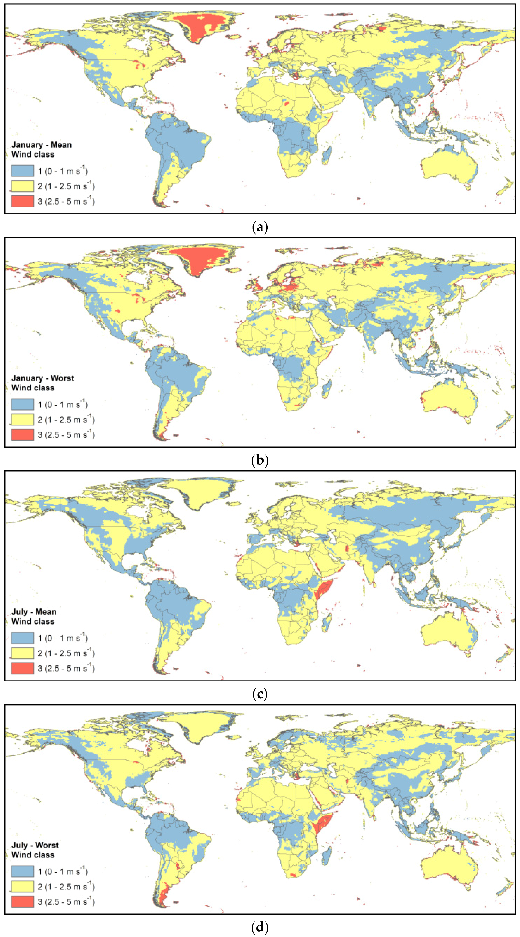
Figure 6 shows the wind classes applied to the computation of fire behavior, both for January and July, and for the mean and worst-case scenarios. The main differences between these two months when considering the mean environmental conditions were the higher wind classes in the Northern Hemisphere during January (Figure 6a), including North America, Russia and Japan, and an increase of the wind class in July in north-eastern Brazil, eastern Africa and the Middle East (Figure 6c). There was no significant difference in the wind class patterns in January between the mean and worst-case scenarios apart from some wind class increases from 1 to 2 near the tropics. But during July (Figure 6d) an increase of wind class 2 was noticeable in North America and Russia, as well as eastern Brazil, while the winds decreased in the Scandinavian Peninsula. There was also an increase of class-3 winds in the Patagonian region of South America.
As previously indicated, the “worst-case scenario” wind classes did not correspond to the maximum winds, but to the average winds found for the 30 days with the lowest FMC of the study period.
3.2. Fire Behavior
Figure 7, Figure 8 and Figure 9 show the results of the fire behavior simulations obtained for January and July both for the average and most extreme conditions during the study period. The results for the rest of the months are shown in the Supplementary Materials (Tables S3 to S5) to this article.
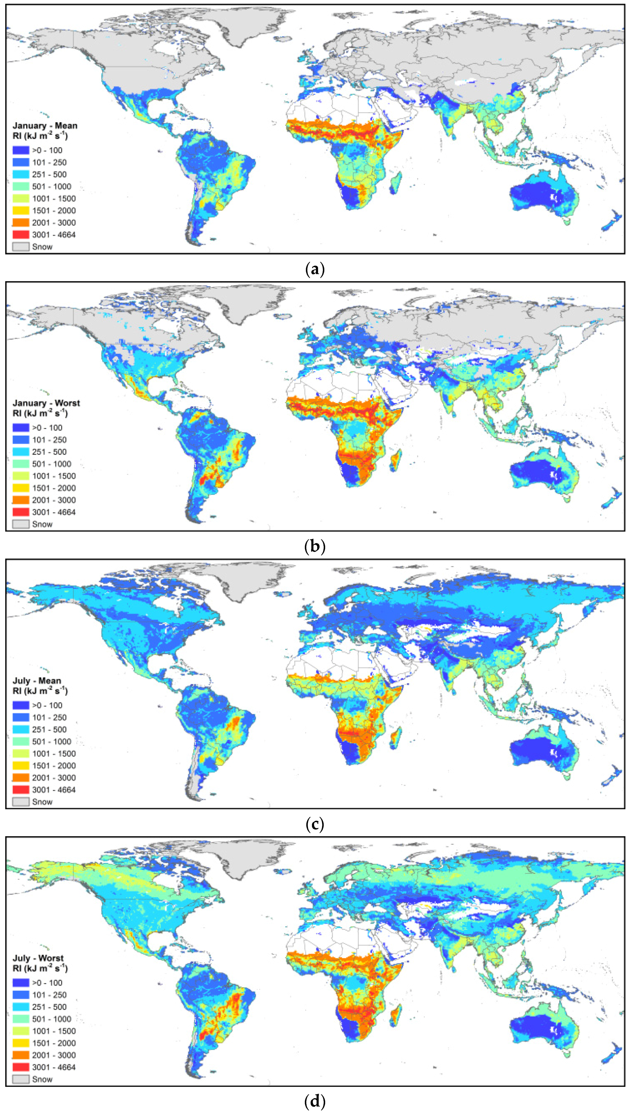
The predicted reaction intensity had values as high as 4664 kJ·m−2·s−1 both in the January mean conditions (Figure 7a) and worst-case scenario (Figure 7b). During this month, when mean environmental conditions were simulated, the values of RI higher than 3000 kJ·m−2·s−1 were all located in Sub-Saharan Africa. Regarding July, the highest RI value obtained for the mean conditions (Figure 7c) was of 3835 kJ·m−2·s−1, located in Zambia, and the worst-case scenario (Figure 7d) was located in Argentina, with a value of 4435 kJ·m−2·s−1. The global distribution of cells with values of RI higher than 3000 kJ·m−2·s−1 for the extreme environmental conditions were similar both in January and July, covering shrubland and savanna regions in Northern and Southern Africa, as well as some regions in South America. On the contrary, on mean environmental conditions the highest RI values moved from the Northern to the Southern sub-tropical regions, which can be appreciated in Figure 7a,c.
The highest rate of spread in the 0.5° cells found for the mean conditions in January (Figure 8a) was of 0.567 m·s−1. All the cells with this value were located in the grassland regions of sub-Saharan Africa. When the worst-case scenario was considered (Figure 8b), the highest ROS increased to 0.863 m·s−1, located in South Africa, in the border with Lesotho. In addition, 334 cells had values of ROS higher than 0.5 m·s−1, mostly located in the grassland regions close to the Sahara and Kalahari deserts, with some cells also located in the Mexican Sonoran and Chihuahuan deserts.
During July, the mean environmental conditions (Figure 8c) resulted in the highest ROS of 0.723 m·s−1, located in Somalia. The cells with ROS higher than 0.5 m·s−1 (152 in total) were located in Somalia, Namibia and Botswana north to the Kalahari Desert, eastern Mali, the US Sonoran and Mojave deserts and Southern Kazakhstan. In the case of July’s extreme conditions (Figure 8d), the ROS reached a value of 1.013 m·s−1 in Somalia, and a total of 359 cells had values higher than 0.5 m·s−1. Adding to the regions described for the mean conditions, other desertic or steppe regions in North America and eastern Africa, as well as the rice croplands in southern Kazakhstan, also reached those high values of ROS.
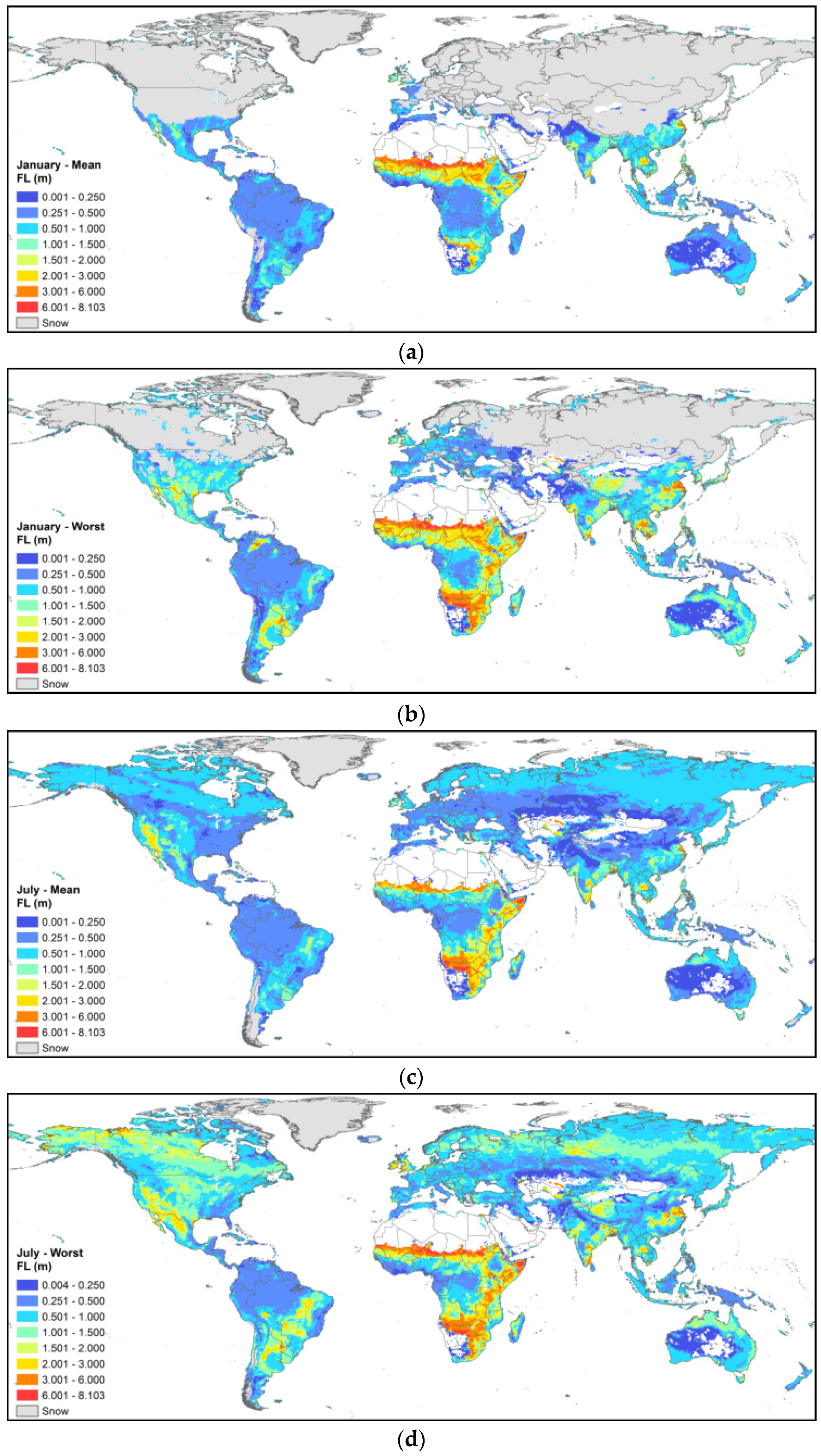
Regarding flame length, the highest values obtained (>6 m) were all located in Africa. The FL values for January reached a value of 6.51 m during mean environmental conditions (Figure 9a), and were located in the grasslands and steppes of Sub-Saharan Africa. All the cells with FL values higher than 6 m were located in that region or Somalia. The highest FL value of the January worst-case scenario (Figure 9b) increased to 7.37 m, and as with the ROS, was located in the border between South Africa and western Lesotho. All cells with FL higher than 6 m were located in the steppes close to the Saharan and Kalahari deserts, and in northern Somalia. During July, the highest value of FL found during the mean conditions (Figure 9c) was 6.76 m in Somalia, and all cells with values higher than 6 m were found there, in Namibia, Botswana or Mali. When the most extreme environmental conditions during July were considered (Figure 9d), the FL reached a value of 8.1 m, with a similar geographical distribution as in the case of January.
The results also show that in several regions of the world with the same environmental conditions, the results of the fire behavior simulation varied only due to the characteristics of the fuels. For example, during July’s mean environmental conditions, the region of the South American Pampas and Gran Chaco (covering Argentina, Uruguay, Paraguay and Southern Brazil) had an environmental scenario 4421, corresponding to a humid fuel moisture scenario, with intermediate winds and low slope (see Table 4). In that scenario, the fuelbed corresponding to forage croplands in a Tropical and Sub-tropical Moist Broadleaf forest (fuelbed 1018) had an RI of 1153.92 kJ·m−2·s−1, an ROS of 0.32 m·s−1 and an FL of 2.98 m. Pixels nearby and with the same environmental conditions but corresponding to a mosaic of natural vegetation and soybean cropland in a Temperate Grasslands, Savannas and Shrubland biome (8033), on the other hand, had an RI value almost four times lower (305.68 kJ·m−2·s−1), with ROS values 40 times lower (0.008 m·s−1) and FL values more than 7 times lower (0.39 m).
4. Discussion
4.1. Environmental Conditions
Relative humidity, temperature, precipitation and wind speed all influence wildland fire behavior. The fuel moisture scenario (FMS) integrates the different contributions of temperature, relative humidity and precipitation. The shift of the dry FMS (D1L1 and D2L2) with the progression of the months is related to the periods of the year when fires are likely to start and spread, usually referred to as the fire season [58]. In some cases, a dry FMS is mainly related to temperature, as is the case of the temperate and boreal Northern Hemisphere regions, which are generally affected by fires from May to September [59,60]. In other regions, such as the tropics, FMS is coupled with the seasonal cycle of precipitation. In these regions, the Inter-Tropical Convergence Zone determines the dry season, and the subsequent fire season, from November to March north of the equator, and from June to October in the Southern Tropical belt (see for example Figure 7 of [59]). This cycle is clearly visible in Figure 5a,c over Africa (and with more detail in Table S1 of the Supplementary Materials), where the humid D4L4 FMS region close to the Equator moves to the south in January, and to the north in July.
In this study, we evaluated the monthly average FMS conditions for the study period (1980–2010), because our objective was to analyze the variability of the fuelbed dataset fire behavior due to changing environmental conditions. But other studies have shown that there has been an increase in the global mean fire weather season length [3] during this period. Still, it is when a set of weather extremes coexist, as in the case of hot, dry and windy conditions, that the most severe fires occur [2,3,4]. For this reason, we also calculated the most extreme environmental conditions found in each month of the study period (the worst-case scenario). As shown in the results (see Figure 5), the worst-case scenario extended vastly the regions assigned to dry FMSs compared to the average scenario, and could allow fires to start and spread in locations where ordinary weather conditions would prevent fire occurrence.
Fire behavior, and specially rate of spread, is strongly affected by wind speed and direction, which can vary in time on the order of hours, minutes or even seconds. Wind is also influenced by terrain, fuel depth and overstory vegetation sheltering, decreasing midflame wind speed up to 60% [55]. All these parameters could not be considered at the resolution of the climate information (0.5°) or even the fuelbed map (approx. 300 m). Also, the value used for the calculations is a mean value of all daily instantaneous values at the time of the climatic data. For this reason, wind speed classes were included as a general variable that identifies regions of the globe with tendencies to have higher wind speeds. The values used for the analysis are not expected to be realistic in local fire events, but to introduce a coarse variable showing areas and months in which fire could have a more severe behavior due to general wind speeds being higher than in other regions or months.
Topography, in this case slope, is also an important factor in fire behavior because flames of a fire burning upslope will preheat the fuel in front of the fire by radiation and convection, and this will cause faster spread rates and longer flame lengths [1,61]. The slope assigned in our simulation, as it was based on 1 km pixels, did not represent local conditions of topography, but roughly characterized height variability of different regions. As in the case of wind speed, this variable was intended to identify regions of the world that could have more severe fire events due to terrain conditions.
4.2. Fire Behavior
The fire behavior estimations were calculated assigning the environmental variables to the existing fuelbeds of Figure 2. These fuelbeds were created using land cover information, mainly the GlobCover v2.2 [62], and the Olson biome’s map [63], and that means that the limitations and uncertainties of those products were carried to the fuelbed map and affected the fire behavior outputs.
For example, the different fire behavior maps showed some abrupt changes in fire behavior in some regions of the world, most noticeably in the limits between south-western Africa and the surrounding regions. That boundary represents the limit between the Desert and Xeric Shrubland biome (biome 13) and the Tropical and Subtropical Grassland, Savannas and Shrublands of the Olson Biomes’ map (biome 7). Each fuelbed in the different biomes had different parameters assigned, such as plant species, fuel loading, percent of vegetation cover, etc., that were dependent on land cover information. As explained by Pettinari and Chuvieco [30], the limits of the different biomes in the Olson map are abrupt, and do not reflect the mosaics and ecotones that determine the gradual transition of vegetation cover between biomes [64]. This caused in some cases that adjacent pixels of a biome boundary had very different parameters in the fuelbed map, and this in turn caused that the fire behavior results were much different on either side of that boundary.
Another example of this geographical boundary problem is the high values of fire behavior parameters obtained in Somalia. That region is comprised mainly by grassland fuelbed pixels, as that was the land cover of the GlobCover product. Other land cover products, such as the GLC2000 land cover map [65] or the hybrid land cover map [66], assigned that region mostly to sparse vegetation cover, in the case of the GLC2000, or to barren lands in the hybrid map, showing that there might be an error of land cover classification in that area. Also, most of the region of northern Somalia, with the exception of the coasts, is allocated by Olson et al. [63] to biome 7. The combination of these factors derived in that region having a tropical grassland fuelbed assigned, which had some of the highest values of fire behavior parameters (see the following discussion), although those results are most probably wrong.
Fire behavior parameters are important because they allow understanding of the fire itself, and not only classifying fire as a binary event (fire–no fire). Fire events are extremely variable, and they produce different effects in the ecosystem. For this reason, the study of the characteristics of fire events, by means of estimating fire behavior parameters, can help in identifying combinations of land cover and environmental conditions that could cause severe fires with relevant environmental impacts, thus posing a higher danger. Additional considerations on the different fire behavior outputs are included in the following paragraphs.
The reaction intensity is an important fire behavior variable because it is related to fire effects, especially to burn severity, including vegetation mortality and consumption of organic soil layers [67]. This could have ecosystem responses such as soil erosion, changes in vegetation composition, etc. The RI value is calculated in FCCS as the sum of component reaction intensities for all surface strata (shrubs, herbaceous vegetation, woody fuels and litter, lichen and moss). Calculations of RI are dependent on intrinsic fuel properties, including live and dead fuel moisture content and flammability, and are not influenced by wind or slope class [68]. Regarding the fuelbeds, the ones with the highest RI corresponded to shrubs located in Tropical and Sub-tropical dry biomes (fuelbeds 2130, 3130 and 7130 of Figure 2). These shrubs presented the highest RI values because they were related to flammable species that contribute to reaction intensity (species that have extractives that provide a ready source of combustible volatiles) and had a higher biomass (available fuel) than other fuel strata such as herbs or small woody fuels in the same biomes. RI is heavily dependent on FMC, as can be observed when comparing Figure 5 and Figure 6. For example, when comparing mean environmental conditions in southern Mali, the 0.5° cells with RI values of around 1500 kJ·m−2·s−1 in July (when the FMS was D3L3) increased to approximately 4000 kJ·m−2·s−1 in January, which had FMS D1L1.
The rate of spread is calculated in FCCS as the maximum of the ROS of all surface fuels, which correspond to the ratio of heat source (surface fire energy propagated to unburned fuels) to surface fuel heat sink (energy required to preheat surface fuels) [68]. The maximum ROS is dependent on the reaction intensity, the biomass (fuel loading), depth, particle density, percent cover, and surface-area-to-volume ratio of small fuels. It is also affected by fuel moisture content (included in the FMS), as it modifies the heat of ignition, which is part of the heat sink. The obtained ROS is then increased by means of wind and slope coefficients that modify the heat source term. This means that the three environmental components affected the resulting ROS. The highest values of rate of spread were found in cells covered mostly by grasses or crops in dry environments, such as grasses in the Tropical and Subtropical grasslands, savannas or shrublands biome (fuelbed 7140) and rice crops in the Desert or Xeric Shrubland biome (fuelbed 13,011), followed by shrublands in the desert biome (13,130). These high ROS values were expected in grasslands because they have a high heat source and relatively low heat sink (low loading), which results in high rates of spread. The FMS had a very large influence in the values of ROS. To cite an example, a 0.5° cell in northeastern Namibia, covered mostly by fuelbed 7140, had an ROS of 0.045 m·s−1 during the mean conditions in January. That cell corresponded to FMS D4L4 during that month, a humid moisture scenario that prevents fire from spreading rapidly due to the high water content of the live and dead vegetation. But with the progression of the months the FMS decreased up to the D1L1 FMS observed during July, and that low fuel moisture content resulted in an ROS of 0.51 m·s−1, more than ten times higher than for January, for the same cell and the same wind class.
As mentioned in the previous section, wind speed had also a large influence in the value of ROS. This can be seen when comparing Figure 7c and Figure 8c in the African tropics: the shape of the border between wind classes 1 and 2 was replicated with a visible increase of ROS in the areas with wind class 2. As a more specific example, the pixels corresponding to grasslands in the Nugaal Valley region in Somalia (fuelbed 7140) with FMS D2L2 and wind class 2 during January mean conditions had an ROS of 0.33 m·s−1, but that value rose to 0.74 m·s−1 in July’s mean conditions, with the same FMS but wind class 3. It has also been mentioned in the previous section that the temporal and spatial resolution of the wind information did not allow calculating realistic values of midflame wind speed. For this reason, the simulated values of ROS maintain the uncertainty associated to the wind information, and should be used with caution. In the particular case of Somalia the ROS values are probably also too high due to the misallocation of the fuelbed in that region, as explained earlier in this section, but it served as a good example of the contribution of winds to the ROS.
As stated at the beginning of Section 2, flame length is the distance between the flame tip and the midpoint of the flame depth at the base of the flame [42]. Under no-wind, no-slope conditions, it is the same as the flame height [1]. FL is calculated in FCCS as the product of the reaction intensity and the rate of spread, and also includes information on the surface-to-volume ratio of the fuelbeds [68]. As such, the influence of the FMS was higher than in the rate of spread results, as it affected both the ROS and the RI parameters, while the wind class and slope class affected only the ROS parameter. The highest values of FL were found in cells dominated by grasslands in tropical dry biomes, following a similar pattern as the ROS values, but there was also a significant contribution of cells dominated by shrublands. As mentioned in the results, all cells with FL higher than 6 m were located in Africa. Although some other regions of the world presented high values of FL, between 3 and 6 m, they did not reach the African values because the fuel and environmental condition combinations did not replicate the African conditions. In South America, for example, the driest FMS calculated for the tropical fuels was D2L2, versus the even dryer D1L1 calculated for Africa. In Asia and North America, on the other hand, although FMS D1L1 was obtained for regions covered by rice fields in Kazakhstan and China, or by shrublands in the North American deserts, those fuelbeds did not have the sufficient fuel loads to result in as high FL values as the tropical grasslands and shrublands in Africa.
It must be noted that all the flame length results pertained to surface fires, that is, to fires that spread over the surface fuels (herbs, shrubs, small (0 to 7.6 cm diameter) dead woody fuels deposited in the ground, litter, lichen and moss), and do not ignite the tree canopies. This is why the highest FL values are found in grasslands and savannas, and the forests have lower FL values even in flammable fuelbeds such as the needle-leaved temperate and boreal forests, where FL corresponded only to the understory and dead ground fuels loadings. This is because the modified Rothermel spread model within FCCS was designed only to predict surface fire behavior. But much higher flame heights can occur when the fire spreads to the canopies, reaching heights of two or three times the canopy height [69]. Although FCCS calculates a Crown Fire Potential, which ranks the different fuels according to whether they provide sufficient energy to ignite and sustain fire spread in the canopy [68], this potential is based only on the fuel characteristics and it is not affected by the environmental conditions. For this reason, this output was not analyzed in this article.
Flame length could be used as an alternative measure of fireline intensity (FI), as it is proportional to this parameter. FI is the amount of heat released per unit of fire front and per second [70], and it is related to the difficulty of containment of a fire [1]. For this reason, FI (derived from FL) could be used as an indirect measure of fire danger, as has been done in other projects, such as Chuvieco et al. [71]. FI is also related to the severity of the fire, and has been used by various authors to evaluate the effects of the fire over the ecosystem [67], such as dynamics of the tree layer [72] or initiation of crown fires [73].
It should be taken into consideration that the expected fire behavior parameters shown in the results do not mean that with higher values of ROS, FL or RI a fire will actually occur. This article addressed both the climatic and the fuel variables that influence fire occurrence, but did not incorporate information regarding sources of ignition. An ignition source is necessary for a fire to start, and if it does, the availability of fuels and their fuel moisture content must allow the fire to be maintained. After this first step, the fire behavior will be more severe with lower FMC and higher wind speeds and slopes [1]. For this reason, fire is expected to be more severe in the months of the year when conditions are dryer, and with fuels that have properties that increase fire spread and severity.
As it has been commented in the previous paragraphs, the resolution of the data (from approx. 300 m of the fuelbed map, to the 0.5 degrees of the climatological information) allows producing only coarse resolution fire behavior outputs. Also, the fuelbed characteristics assignment, being based on mean global information [30], derived in a generalization of those characteristics, which in reality vary widely across the landscape. As such, they will not represent realistic conditions at a local scale (for example, a particular plot or city). On the other hand, we consider that the fire behavior outputs could provide information to identify regions and seasons of the world with higher fire danger as those which would cause more severe fire behavior events. For example, these kinds of results, coupled with weather forecasts, could provide information for large-scale fire management, such as provisions for fire suppression resource exchanges between provinces or countries. They could also improve the fire risk assessment of systems based solely on weather variables, with the incorporation of the variables associated to the fuel characteristics.
The coarse resolution of the climatic and topographic data and the intrinsic limitations of the Global Fuelbed Dataset do not allow a direct validation of the results. As an alternative method to assess the fire behavior simulation, future work will compare the reaction intensity results with other sources of fire radiative energy, such as the MODIS MYD14 of Thermal Anomalies [74,75]. Also, a statistical analysis of local fire behavior information from different parts of the world could be used to evaluate the general fit of our simulations.
5. Conclusions
This study presented a global fire behavior simulation based on a global fuelbed dataset and climatic and topographic information. The simulation was executed using the Fuel Characteristic Classification System, which uses a reformulation of the Rothermel fire behavior model, and allows calculating surface fire behavior parameters. The climatic information covered the period 1980–2010, and daily weather parameters were used to calculate the mean monthly fuel moisture content and wind speed for the early afternoon period. Also, as the most severe fires occur with extreme environmental conditions, a worst-case scenario was created using the mean value of the 30 days with lowest FMC during each month of the study period. The FMC and wind speed information was grouped into classes, and FCCS was used to simulate the reaction intensity, rate of spread and flame length of the fuelbeds in the different environmental conditions. These results were then mapped, showing the variations in surface fire behavior during the different months of the year throughout the world, both due to the climatic conditions and the characteristics of the fuels.
The maps showed that the highest values of reaction intensity were found in shrubland fuelbeds in tropical and sub-tropical dry regions, the highest rates of spread were obtained for grasslands in those locations and shrublands in desertic areas, and the highest flame lengths occurred in African savannas. All parameters were highly affected by the environmental conditions, increasing their values up to an order of magnitude with changes in the fuel moisture content of the fuels, but the parameters also varied within the same environmental conditions due only to fuel characteristics.
The coarse resolution of the climatic data, though providing information on regional weather conditions, cannot allow an accurate prediction of local fire behavior, because local conditions of fuel moisture and wind can rapidly change and modify the fire behavior, and also fuels vary widely across the landscape. Still, the results show the importance of including detailed fuel information into fire risk assessment systems based on weather parameters, as it could help to better estimate the expected fire behavior and effects.
Supplementary Materials
The following are available online at www.mdpi.com/1999-4907/8/6/179/s1, Table S1: Monthly Fuel Moisture Scenarios, Table S2: Monthly Wind Classes, Table S3: Monthly Reaction Intensity, Table S4: Monthly Rate of Spread, Table S5: Monthly Flame Length.
Acknowledgments
The authors thank Susan Prichard, Anne Andreu and Paige Eagle for their help and support in the use of FCCS, and Roger Ottmar for his suggestions in the definition of the environmental thresholds.
Author Contributions
M. L. Pettinari and E. Chuvieco designed the study. M. L. Pettinari performed the calculations, analyzed the data and wrote the manuscript. E. Chuvieco contributed to the analysis of the data and reviewed the manuscript.
Conflicts of Interest
The authors declare no conflict of interest.
References
- Rothermel, R.C. How to Predict the Spread and Intensity of Forest and Range Fires; INT-143; National Wildfire Coordinating Group, USDA Forest Service Intermountain Research Station: Boise, ID, USA, 1983; p. 166.
- Achard, F.; Eva, H.D.; Mollicone, D.; Beuchle, R. The effect of climate anomalies and human ignition factor on wildfires in Russian boreal forests. Philos. Trans. R. Soc. Lond. B Biol. Sci. 2008, 363, 2331–2339. [Google Scholar] [CrossRef] [PubMed]
- Jolly, W.M.; Cochrane, M.A.; Freeborn, P.H.; Holden, Z.A.; Brown, T.J.; Williamson, G.J.; Bowman, D.M.J.S. Climate-induced variations in global wildfire danger from 1979 to 2013. Nat. Commun. 2015, 6, 7537. [Google Scholar] [CrossRef] [PubMed]
- Flannigan, M.D.; Harrington, J.B. A study of the relation of meteorological variables to monthly provincial area burned by wildfire in Canada (1953–1980). J. Appl. Meteorol. 1988, 27, 441–452. [Google Scholar] [CrossRef]
- Flannigan, M.D.; Stocks, B.J.; Wotton, B.M. Climate change and forest fires. Sci. Total Environ. 2000, 262, 221–229. [Google Scholar] [CrossRef]
- Flannigan, M.; Cantin, A.S.; de Groot, W.J.; Wotton, M.; Newbery, A.; Gowman, L.M. Global wildland fire season severity in the 21st century. For. Ecol. Manag. 2013, 294, 54–61. [Google Scholar] [CrossRef]
- De Groot, W.J.; Flannigan, M.D.; Cantin, A.S. Climate change impacts on future boreal fire regimes. For. Ecol. Manag. 2013, 294, 35–44. [Google Scholar] [CrossRef]
- Andrews, P.L.; Bevins, C.D.; Seli, R.C. BehabePlus Fire Modeling System Version 4.0. User Guide.; RMRS-GTR-106WWW; USDA Forest Service, Rocky Mountain Research Station: Fort Collins, CO, USA, July 2008; p. 123. [Google Scholar]
- Cohen, J.D.; Deeming, J.E. The National Fire-Danger Rating System: Basic Equations; General Technical Report PSW-82; USDA Forest Service, Pacific Southwest Forest and Range Experiment Station: Berkeley, CA, USA, 1985; p. 23. [Google Scholar]
- Stocks, B.J.; Lawson, B.D.; Alexander, M.E.; Van Wagner, C.E.; McAlpine, R.S.; Lynham, T.J.; Dubé, D.E. Canadian Forest Fire Danger Rating System: An overview. For. Chron. 1989, 65, 258–265. [Google Scholar] [CrossRef]
- Ottmar, R.D.; Sandberg, D.V.; Riccardi, C.L.; Prichard, S.J. An overview of the Fuel Characteristic Classification System—Quantifying, classifying, and creating fuelbeds for resource planning. Can. J. For. Res. 2007, 37, 2383–2393. [Google Scholar] [CrossRef]
- Scott, J.H.; Burgan, R.E. Standard Fire Behavior Fuel Models: A Comprehensive Set for Use with Rothermel's Surface Fire Spread Model; RMRS-GTR-153; USDA Forest Service, Rocky Mountain Research Station: Fort Collins, CO, USA, 2005; p. 80. [Google Scholar]
- Cheyette, D.; Rupp, T.S.; Rodman, S. Developing Fire Behavior Fuel Models for the Wildland-Urban Interface in Anchorage, Alaska. West. J. Appl. For. 2008, 23, 149–155. [Google Scholar]
- Elia, M.; Lafortezza, R.; Lovreglio, R.; Sanesi, G. Developing Custom Fire Behavior Fuel Models for Mediterranean Wildland–Urban Interfaces in Southern Italy. Environ. Manag. 2015, 56, 754–764. [Google Scholar] [CrossRef] [PubMed]
- Zhi, W.W.; Hong, S.H.; Yu, C.; Zhi, H.L.; Hong, W.C. Development of customized fire behavior fuel models for boreal forests of Northeastern China. Environ. Manag. 2011, 48, 1148–1157. [Google Scholar]
- De Groot, W.J.; Goldammer, J.G.; Keenan, T.; Brady, M.A.; Lynham, T.J.; Justice, C.O.; Csiszar, I.A.; O’Loughlin, K. Developing A Global Early Warning System for Wildland Fire. In Proceedings of the V International Conference on Forest Fire Research, Coimbra, Portugal, 27–30 November 2006. [Google Scholar]
- San Miguel-Ayanz, J.; Schulte, E.; Schmuck, G.; Camia, A.; Strobl, P.; Liberta, G.; Giovando, C.; Boca, R.; Sedano, F.; Kempeneers, P.; et al. Comprehensive Monitoring of Wildfires in Europe: The European Forest Fire Information System (EFFIS). In Approaches to Managing Disaster—Assessing Hazards, Emergencies and Disaster Impacts; Tiefenbacher, J., Ed.; InTech: Rijeka, Croatia, 2012; pp. 87–108. [Google Scholar]
- Van Wagner, C.E. Development and Structure of the Canadian Forest Fire Weather Index System; Canadian Forestry Service: Ottawa, ON, Canada, 1987; p. 37. [Google Scholar]
- EFFIS—European Forest Fire Information System. Fire Danger Forecast Technical Background. Available online: http://effis.jrc.ec.europa.eu/about-effis/technical-background/fire-danger-forecast/ (accessed on 29 April 2017).
- Department of National Parks—Wildlife and Plant Conservation—Thailand. Fine-Resolution Forecast Products of Fire Danger Rating. Available online: http://www2.dnp.go.th/gis/FDRS/FDRS.php (accessed on 30 April 2017).
- Dowdy, A.J.; Mills, G.A.; Finkele, K.; de Groot, W.J. Australian Fire Weather as Represented by the McArthur Forest Fire Danger Index and the Canadian Forest Fire Weather Index. Available online: http://www.cawcr.gov.au/technical-reports/CTR_010.pdf (accessed on 13 March 2017).
- Bureau of Meteorology—Australian Government. National Fire Danger Rating System. Available online: http://www.bom.gov.au/weather-services/bushfire/index.shtml (accessed on 30 April 2017).
- Global Early Warning System for Wildland Fires. Available online: http://www.fire.uni-freiburg.de/gwfews/index.html (accessed on 30 April 2017).
- De Groot, W.J.; Goldammer, J.G.; Justice, C.O.; Lynham, T.J.; Csiszar, I.A.; San-Miguel-Ayanz, J. Implementing a Global Early Warning System for Wildland Fire. In Proceedings of the VI International Conference on Forest Fire Research, Coimbra, Portugal, 15–18 Nobember 2010; Viegas, D.X., Ed.; ADAI/CEIF: Coimbra, Portugal, 2010; p. 13. [Google Scholar]
- Copernicus—European Comission. European Forest Fire Information System (EFFIS) and Global Wilfire Information System (GWIS). Available online: http://effis.jrc.ec.europa.eu/effis-gwis/ (accessed on 30 April 2017).
- Joint Research Centre (JRC). Global Wilfire Information System (Beta Viewer). Available online: http://forest.jrc.ec.europa.eu/effis/applications/global-viewer/ (accessed on 30 April 2017).
- Uhl, C.; Kauffman, J.B. Deforestation, fire susceptibility, and potential tree responses to fire in the eastern Amazon. Ecology 1990, 71, 437–449. [Google Scholar] [CrossRef]
- Rogers, B.M.; Soja, A.J.; Goulden, M.L.; Randerson, J.T. Influence of tree species on continental differences in boreal fires and climate feedback. Nat. Geosci. 2015, 8, 228–234. [Google Scholar] [CrossRef]
- De Groot, W.J.; Cantin, A.S.; Flannigan, M.D.; Soja, A.J.; Gowman, L.M.; Newbery, A. A comparison of Canadian and Russian borel forest fire regimes. For. Ecol. Manag. 2013, 294, 23–34. [Google Scholar] [CrossRef]
- Pettinari, M.L.; Chuvieco, E. Generation of a global fuel data set using the Fuel Characteristic Classification System. Biogeosciences 2016, 13, 2061–2076. [Google Scholar] [CrossRef]
- Thurner, M.; Beer, C.; Santoro, M.; Carvalhais, N.; Wutzler, T.; Schepaschenko, D.; Shvidenko, A.; Kompter, E.; Ahrens, B.; Levick, S.R.; et al. Carbon stock and density of northern boreal temperate forests. Glob. Ecol. Biogeogr. 2014, 23, 297–310. [Google Scholar] [CrossRef]
- Yue, C.; Ciais, P.; Cadule, P.; Thonicke, K.; Archibald, S.; Poulter, B.; Hao, W.M.; Hantson, S.; Mouillot, F.; Friedlingstein, P.; et al. Modelling the role of fires in the terrestrial carbon balance by incorporating SPITFIRE into the global vegetation model ORCHIDEE—Part 1: Simulating historical global burned area and fire regimes. Geosci. Model. Dev. 2014, 7, 2747–2767. [Google Scholar] [CrossRef]
- Saatchi, S.S.; Harris, N.L.; Brown, S.; Lefsky, M.A.; Mitchard, E.T.A.; Salas, W.; Zutta, B.R.; Buermann, W.; Lewis, S.L.; Hagen, S.; et al. Benchmark map of forest carbon stocks in tropical regions across three continents. PNAS 2011, 108, 9899–9904. [Google Scholar] [CrossRef] [PubMed]
- Baccini, A.; Goetz, S.J.; Walker, W.S.; Laporte, N.T.; Sun, M.; Sulla-Menashe, D.; Hackler, J.; Beck, P.S.A.; Dubayah, R.; Friedl, M.A.; et al. Estimated carbon dioxide emissions from tropical deforestation improved by carbon-density maps. Nat. Clim. Chang. 2012, 2, 182–185. [Google Scholar] [CrossRef]
- Pettinari, M.L.; Chuvieco, E. Cartografía de combustible y potenciales de incendio en el continente africano utilizando FCCS. Rev. Teledetec. 2015, 43, 1–10. [Google Scholar] [CrossRef]
- Pettinari, M.L.; Ottmar, R.D.; Prichard, S.J.; Andreu, A.G.; Chuvieco, E. Development and mapping of fuel characteristics and associated fire potentials for South America. Int. J. Wildland Fire 2014, 23, 643–654. [Google Scholar] [CrossRef]
- Dee, D.P.; Uppala, S.M.; Simmons, A.J.; Berrisford, P.; Poli, P.; Kobayashi, S.; Andrae, U.; Balmaseda, M.A.; Balsamo, G.; Bauer, P.; et al. The ERA-Interim reanalysis: configuration and performance of the data assimilation system. Q. J. R. Meteorol. Soc. 2011, 137, 553–597. [Google Scholar] [CrossRef]
- Riccardi, C.L.; Ottmar, R.D.; Sandberg, D.V.; Andreu, A.; Elman, E.; Kopper, K.; Long, J. The fuelbed: A key element of the Fuel Characteristic Classification System. Can. J. For. Res. 2007, 37, 2394–2412. [Google Scholar] [CrossRef]
- Sandberg, D.V.; Riccardi, C.L.; Schaaf, M.D. Fire potential rating for wildland fuelbeds using the Fuel Characteristic Classification System. Can. J. For. Res. 2007, 37, 2456–2463. [Google Scholar] [CrossRef]
- Rothermel, R.C. A Mathematical Model for Predicting Fire Spread in Wildland Fuels; Research Paper INT-115; USDA Forest Service, Intermountain Forest and Range Experiment Station: Odgen, UT, USA, 1972; p. 40. [Google Scholar]
- Sandberg, D.V.; Riccardi, C.L.; Schaaf, M.D. Reformulation of Rothermel’s wildland fire behaviour model for heterogeneous fuelbeds. Can. J. For. Res. 2007, 37, 2438–2455. [Google Scholar] [CrossRef]
- Albini, F.A. Estimating Wildfire Behavior and Effects; General Technical Report INT-30; USDA Forest Service, Intermountain Forest and Range Experiment Station: Odgen, UT, USA, 1976; p. 92. [Google Scholar]
- DiMiceli, C.M.; Carroll, M.L.; Sohlberg, R.A.; Huang, C.; Hansen, M.C.; Townsend, J.R.G. Vegetation Continuous Field (MOD44B), Collection 5 Percent Tree Cover, Collection 5th ed.; University of Maryland, College Park: College Park, MD, USA, 2011. [Google Scholar]
- Global Land Cover Facility. MODIS Vegetation Continuous Field. Available online: http://glcf.umd.edu/data/vcf/ (accessed on 11 May 2017).
- Simard, M.; Pinto, N.; Fisher, J.B.; Baccini, A. Mapping forest canopy height globally with spaceborne lidar. J. Geophys. Res. 2011, 116, 12. [Google Scholar] [CrossRef]
- Morfín-Ríos, J.E.; Alvarado-Celestino, E.; Jardel-Peláez, E.J.; Vihnanek, R.E.; Wright, D.K.; Michel-Fuentes, J.M.; Wright, C.S.; Ottmar, R.D.; Sandberg, D.V.; Nájera-Díaz, A. Photo Series for Quantifying Forest Fuels in Mexico: Montane Subtropical Forests of the Sierra Madre del Sur and Temperate Forests and Montane Shrubland of the Northern Sierra Madre Oriental; Pacific Wildland Fire Sciences Laboratory Special Pub. No. 1; University of Washington, College of Forest Resources: Seattle, WA, USA, 2008; p. 93. [Google Scholar]
- Ottmar, R.D.; Vihnanek, R.E.; Miranda, H.S.; Sato, M.N.; Andrade, S.M.A. Stereo Photo Series for Quantifying Cerrado Fuels in Central Brazil; General Technical Report PNW-GTR-519; USDA Forest Service, Pacific Northwest Research Station: Seattle, WA, USA, 2001; Volume 1, p. 88. [Google Scholar]
- Pettinari, M.L. Global Fuelbed Dataset. Available online: http://doi.pangaea.de/10.1594/PANGAEA.849808 (accessed on 13 March 2017).
- ECMWF Datasets. Available online: http://www.ecmwf.int/en/forecasts/datasets (accessed on 13 March 2017).
- Balsamo, G.; Albergel, C.; Beljaars, A.; Boussetta, S.; Brun, E.; Cloke, H.; Dee, D.; Dutra, E.; Muñoz-Sabater, J.; Pappenberger, F.; et al. ERA-Interim/Land: A global land surface reanalysis data set. Hydrol. Earth Syst. Sci. 2015, 19, 389–407. [Google Scholar] [CrossRef]
- ERA-20CM Model Integrations. Available online: http://www.ecmwf.int/en/research/climate-reanalysis/era-20cm-model-integrations (accessed on 13 March 2017).
- ERA-20C. Available online: http://www.ecmwf.int/en/research/climate-reanalysis/era-20c (accessed on 13 March 2017).
- Global 30 Arc-Second Elevation (GTOPO30). Available online: https://lta.cr.usgs.gov/GTOPO30 (accessed on 13 March 2017).
- Wanielista, M.; Kersten, R.; Eaglin, R. Hydrology: Water Quantity and Quality Control, 2nd ed.; Wiley: New York, NY, USA, 1997. [Google Scholar]
- Andrews, P.L. Modeling Wind Adjustment Factor and Midflame Wind Speed for Rothermel’s Surface Fire Spread Model; Gen. Tech. Rep. RMRS-GTR-266; USDA Forest Service, Rocky Mountain Research Station: Fort Collins, CO, USA, 2012; p. 39. [Google Scholar]
- Turner, J.A.; Lawson, B.D. Weather in the Canadian Forest Fire Danger Rating System: A User’s Guide to National Standards and Practices; Information Report BC-X-177; Canadian Forest Service, Pacific Forest Research Centre: Victoria, BC, Canada, 1978; p. 40. [Google Scholar]
- Fuel and Fire Tools. Available online: https://www.fs.fed.us/pnw/fera/fft/index.shtml (accessed on 13 March 2017).
- Merrill, D.F.; Alexander, M.E. Glossary of Forest Fire Management Terms; NRCC No 26516; Canadian Committee on Forest Fire Management, National Research Council of Canada: Ottawa, ON, Canada, 1987; p. 57.
- Alonso-Canas, I.; Chuvieco, E. Global burned area mapping from ENVISAT-MERIS and MODIS active fire data. Remote Sens. Environ. 2015, 163, 140–152. [Google Scholar] [CrossRef]
- Giglio, L.; Csiszar, I.; Justice, C.O. Global distribution and seasonality of active fires as observed with the Terra and Aqua Moderate Resolution Imaging Spectroradiometer (MODIS) sensors. J. Geophys. Res. Biogeosci. 2006, 111, 12. [Google Scholar] [CrossRef]
- Viegas, D.X. Slope and wind effects on fire propagation. Int. J. Wildland Fire 2004, 13, 143–156. [Google Scholar] [CrossRef]
- Bicheron, P.; Defourny, P.; Brockmann, C.; Schouten, L.; Vancutsem, C.; Huc, M.; Bontemps, S.; Leroy, M.; Achard, F.; Herold, M.; et al. GLOBCOVER: Products Description and Validation Report; MEDIAS-France/POSTEL: Toulouse, France, 2008; p. 47. [Google Scholar]
- Olson, D.M.; Dinerstein, E.; Wikramanayake, E.D.; Burgess, N.D.; Powell, G.V.N.; Underwood, E.C.; D’Amico, J.A.; Itoua, I.; Strand, H.E.; Morrison, J.C.; et al. Terrestrial Ecoregions of the World: A New Map of Life on Earth. BioScience 2001, 51, 933–938. [Google Scholar] [CrossRef]
- Walker, S.; Wilson, J.B.; Steel, J.B.; Rapson, G.L.; Smith, B.; King, W.M.; Cottam, Y.H. Properties of ecotones: Evidence from five ecotones objectively determined from a coastal vegetation gradient. J. Veg. Sci. 2003, 14, 579–590. [Google Scholar] [CrossRef]
- Mayaux, P.; Eva, H.; Gallego, J.; Strahler, A.H.; Herold, M.; Agrawal, S.; Naumov, S.; De Miranda, E.E.; Di Bella, C.M.; Ordoyne, C.; et al. Validation of the global land cover 2000 map. IEEE Trans. Geosci. Remote Sens. 2006, 44, 1728–1739. [Google Scholar] [CrossRef]
- See, L.; Schepaschenko, D.; Lesiv, M.; McCallum, I.; Fritz, S.; Comber, A.; Perger, C.; Schill, C.; Zhao, Y.; Maus, V.; et al. Building a hybrid land cover map with crowdsourcing and geographically weighted regression. ISPRS J. Photogramm. Remote Sens. 2015, 103, 48–56. [Google Scholar] [CrossRef]
- Keeley, J.E. Fire intensity, fire severity and burn severity: A brief review and suggested usage. Int. J. Wildland Fire 2009, 18, 116–126. [Google Scholar] [CrossRef]
- Prichard, S.J.; Sandberg, D.V.; Ottmar, R.D.; Eberhardt, E.; Andreu, A.; Eagle, P.; Swedin, K. Fuel Characteristic Classification System Version 3.0: Technical Documentation; PNW-GTR-887; USDA Forest Service, Pacific Norhtwest Research Station: Portland, OR, USA, 2013; p. 88. [Google Scholar]
- Alexander, M.E.; Cruz, M.G. Chapter 9: Crown Fire Dynamics in Conifer Forests; Report PNW-GTR-891; USDA Forest Service, Pacific Northwest Research Station: Portland, OR, USA, 2014; p. 188. [Google Scholar]
- Byram, G.M. Combustion of forest fuels. In Forest Fire Control and Use; Davis, K.P., Ed.; McGraw-Hill Book Co.: New York, NY, USA, 1959; pp. 61–89. [Google Scholar]
- Chuvieco, E.; Aguado, I.; Jurdao, S.; Pettinari, M.L.; Yebra, M.; Salas, J.; Hantson, S.; de la Riva, J.; Ibarra, P.; Rodrigues, M.; et al. Integrating geospatial information into fire risk assessment. Int. J. Wildland Fire 2014, 23, 606–619. [Google Scholar] [CrossRef]
- Govender, N.; Trollope, W.S.W.; Van Wilgen, B.W. The effect of fire season, fire frequency, rainfall and management on fire intensity in savanna vegetation in South Africa. J. Appl. Ecol. 2006, 43, 748–758. [Google Scholar] [CrossRef]
- Alexander, M.E.; Cruz, M.G. Interdependencies between flame length and fireline intensity in predicting crown fire initiation and crown scorch height. Int. J. Wildland Fire 2012, 21, 95–113. [Google Scholar] [CrossRef]
- Thermal Anomalies and Fire Daily L3 Global 1 km. Available online: https://lpdaac.usgs.gov/dataset_discovery/modis/modis_products_table/myd14a1 (accessed on 13 March 2017).
- Wooster, M.J.; Roberts, G.; Perry, G.L.W.; Kaufman, Y.J. Retrieval of biomass combustion rates and totals from fire radiative power observations: FRP derivation and calibration relationships between biomass consumption and fire radiative energy release. J. Geophys. Res. 2005, 110, D24311. [Google Scholar] [CrossRef]
Figure 1.
Summary of the methodology for predicting fire behavior.

Figure 2.
Global fuel map [30].
Figure 2.
Global fuel map [30].
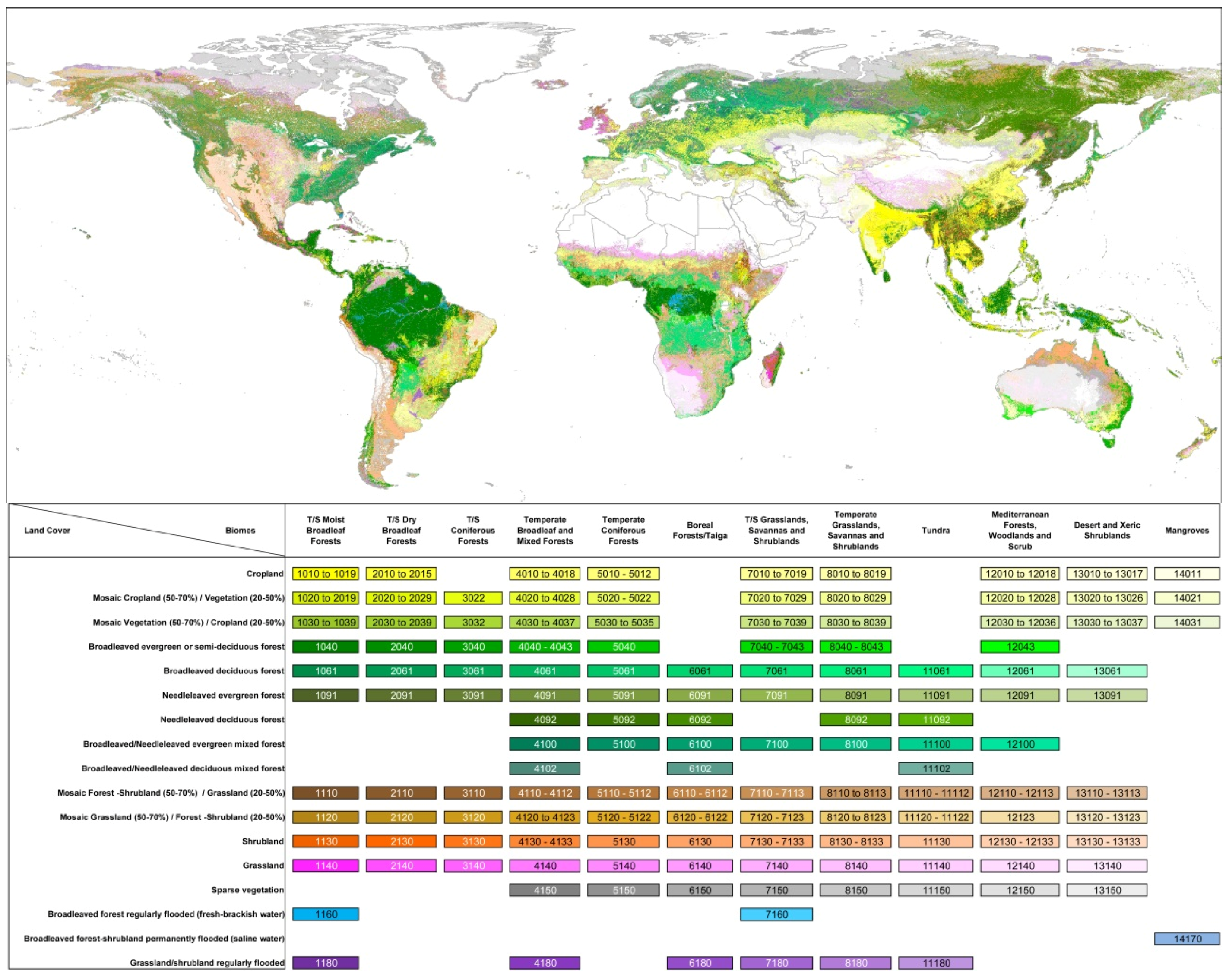
Figure 3.
Longitudinal strips, each corresponding to a time step of climatic data.
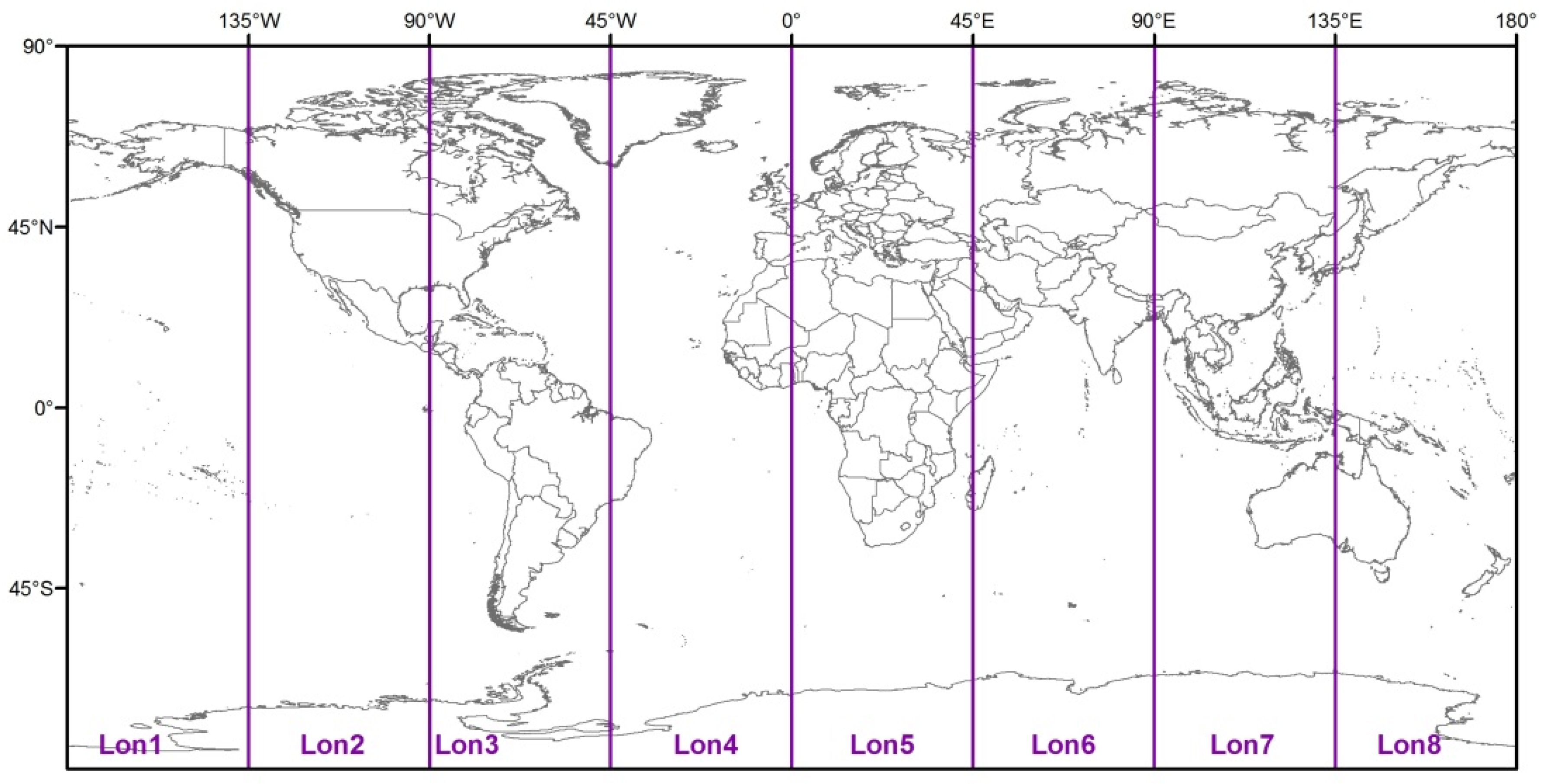
Figure 4.
Slope classes derived from GTOPO30.
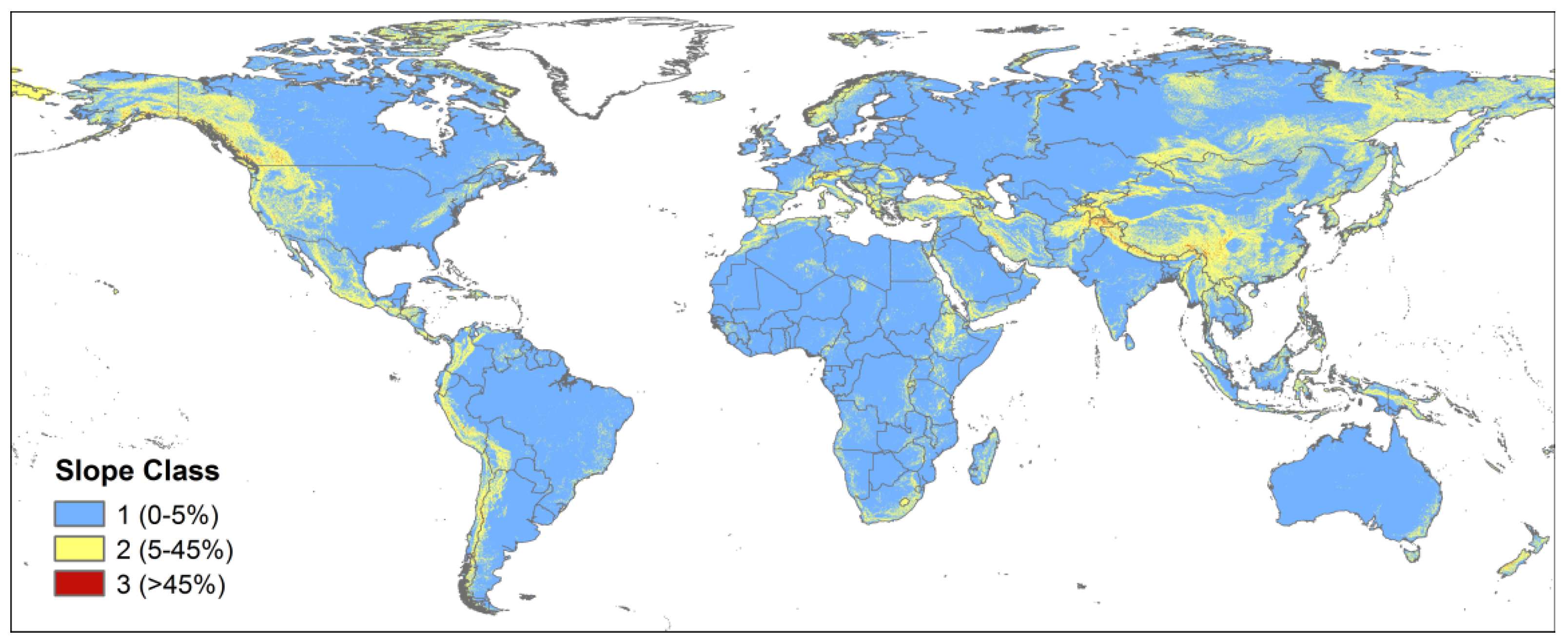
Figure 5.
(a) Fuel Moisture Scenario (FMS) for January reflecting the mean daily conditions; (b) FMS for January with the worst-case scenario for the study period; (c) FMS for July’s mean conditions; and (d) FMS for July’s most extreme conditions. For the fuel moisture content values of each scenario, see Table 3.
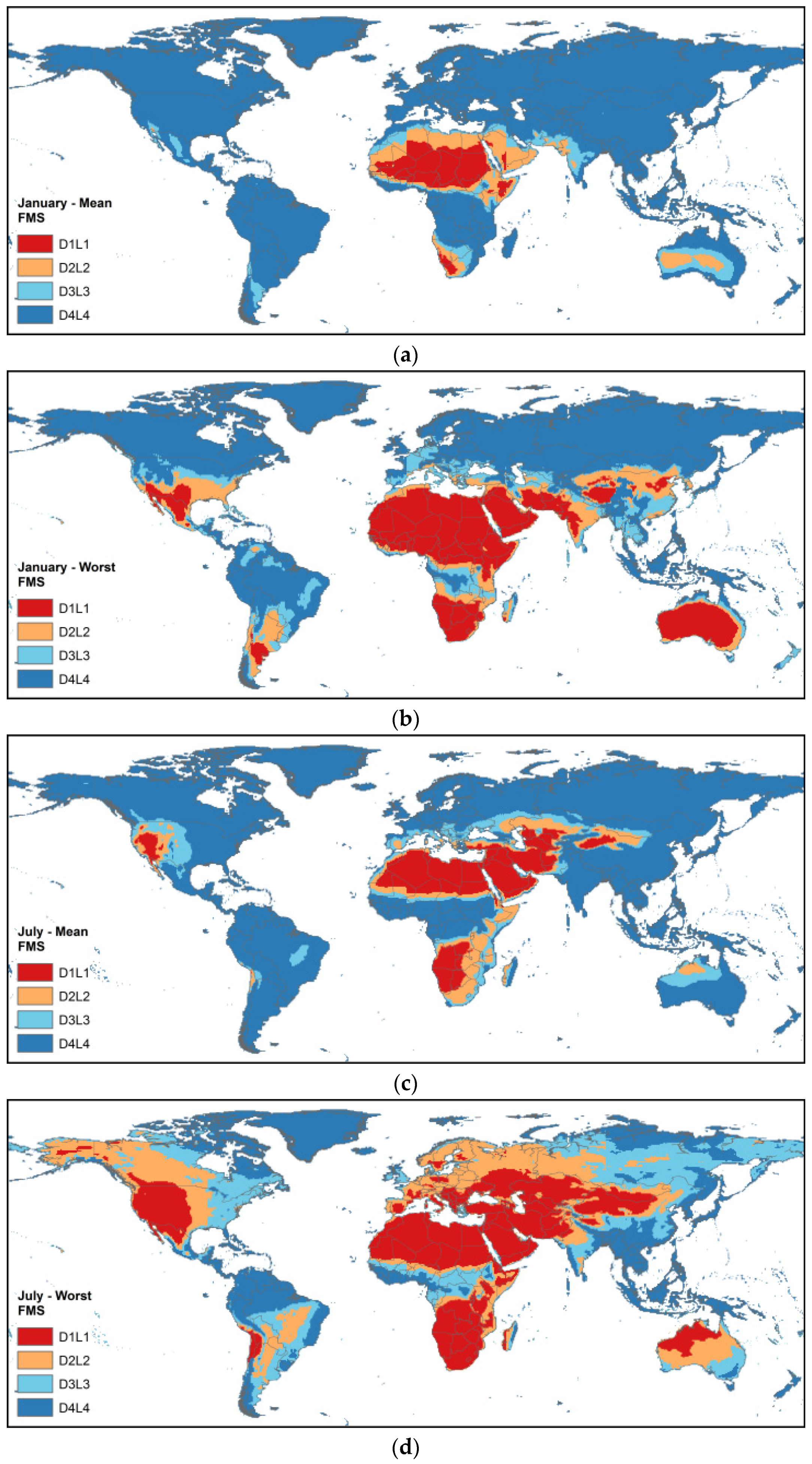
Figure 6.
(a) Wind classes for January reflecting the mean daily conditions; (b) Wind classes for January with the worst-case scenario for the study period; (c) Wind classes for July’s mean conditions; and (d) Wind classes for July’s most extreme conditions.
Figure 6.
(a) Wind classes for January reflecting the mean daily conditions; (b) Wind classes for January with the worst-case scenario for the study period; (c) Wind classes for July’s mean conditions; and (d) Wind classes for July’s most extreme conditions.

Figure 7.
(a) Reaction intensity (RI) for January reflecting the mean daily conditions; (b) RI for January with the worst-case scenario for the study period; (c) RI for July’s mean conditions; and (d) RI for July’s most extreme conditions.
Figure 7.
(a) Reaction intensity (RI) for January reflecting the mean daily conditions; (b) RI for January with the worst-case scenario for the study period; (c) RI for July’s mean conditions; and (d) RI for July’s most extreme conditions.

Figure 8.
(a) Rate of spread (ROS) for January reflecting the mean daily conditions; (b) ROS for January with the worst-case scenario for the study period; (c) ROS for July’s mean conditions; and (d) ROS for July’s most extreme conditions.
Figure 8.
(a) Rate of spread (ROS) for January reflecting the mean daily conditions; (b) ROS for January with the worst-case scenario for the study period; (c) ROS for July’s mean conditions; and (d) ROS for July’s most extreme conditions.

Figure 9.
(a) Flame length (FL) for January reflecting the mean daily conditions; (b) FL for January with the worst-case scenario for the study period; (c) FL for July’s mean conditions; and (d) FL for July’s most extreme conditions.
Figure 9.
(a) Flame length (FL) for January reflecting the mean daily conditions; (b) FL for January with the worst-case scenario for the study period; (c) FL for July’s mean conditions; and (d) FL for July’s most extreme conditions.

Table 1.
Regions comprising 4 hours of climatic data accounting for early afternoon conditions.
| Strip | Longitude | UTC | Forecast Time | Step |
|---|---|---|---|---|
| Lon1 1 | 180–135 W | 0 | 0 | 0 |
| Lon2 | 135–90 W | 3 | 0 | 3 |
| Lon3 | 90–45 W | 6 | 0 | 6 |
| Lon4 | 45–0 W | 9 | 0 | 9 |
| Lon5 | 0–45 E | 12 | 0 | 12 |
| Lon6 | 45–90 E | 15 | 12 | 3 |
| Lon7 | 90–135 E | 18 | 12 | 6 |
| Lon8 | 135–180 E | 21 | 12 | 9 |
1 For Lon1, the precipitations correspond to Forecast Time 12, Step 12 of the previous day.
Table 2.
Climatic variables from the ERA-Interim Reanalysis used for this study.
| Variable Name | Variable Code | Units | Other Information |
|---|---|---|---|
| 10 m U wind component | 165 | m·s−1 | Instantaneous at time step. |
| 10 m V wind component | 166 | m·s−1 | Instantaneous at time step. |
| Total Cloud Cover | 164 | Fraction of cover (0–1) | Instantaneous at time step. |
| Snow Depth | 141 | m of water equivalent | Instantaneous at time step. |
| Total Precipitation | 228 | m of water | Accumulated since the forecast time to the step. |
| 2 m Dew Point | 168 | °K | Instantaneous at time step. |
| 2 m Temperature | 167 | °K | Instantaneous at time step. |
Table 3.
Fuel Moisture Scenarios.
| FMS Code | FMS Description | Fuel Moisture Content (%) | |||||
|---|---|---|---|---|---|---|---|
| Herb | Shrub | Crown 1 | 1 h | 10 h | 100 h | ||
| D1L1 | Very low dead FMC, fully cured herb | 30 | 60 | 60 | 3 | 4 | 5 |
| D2L2 | Low dead FMC, 2/3 cured herb | 60 | 90 | 60 | 6 | 7 | 8 |
| D3L3 | Moderate dead FMC, 1/3 cured herb | 90 | 120 | 120 | 9 | 10 | 11 |
| D4L4 | High dead FMC, fully green herb | 120 | 150 | 150 | 12 | 13 | 14 |
1 The Scott and Burgan original FMSs do not include FMCs for Crown. These data were extracted from the description of the variables inside the FCCS software.
Table 4.
Combination of environmental scenarios for fuelbed conditions.
| Environmental Scenario | FMS Code 1 | Wind 2 | Slope 3 | Environmental Scenario | FMS Code 1 | Wind 2 | Slope 3 |
|---|---|---|---|---|---|---|---|
| 1111 | D1L1 | WC1 | SP 1 | 3311 | D3L3 | WC1 | SP 1 |
| 1112 | D1L1 | WC1 | SP 2 | 3312 | D3L3 | WC1 | SP 2 |
| 1113 | D1L1 | WC1 | SP 3 | 3313 | D3L3 | WC1 | SP 3 |
| 1121 | D1L1 | WC2 | SP 1 | 3321 | D3L3 | WC2 | SP 1 |
| 1122 | D1L1 | WC2 | SP 2 | 3322 | D3L3 | WC2 | SP 2 |
| 1123 | D1L1 | WC2 | SP 3 | 3323 | D3L3 | WC2 | SP 3 |
| 1131 | D1L1 | WC3 | SP 1 | 3331 | D3L3 | WC3 | SP 1 |
| 1132 | D1L1 | WC3 | SP 2 | 3332 | D3L3 | WC3 | SP 2 |
| 1133 | D1L1 | WC3 | SP 3 | 3333 | D3L3 | WC3 | SP 3 |
| 2211 | D2L2 | WC1 | SP 1 | 4411 | D4L4 | WC1 | SP 1 |
| 2212 | D2L2 | WC1 | SP 2 | 4412 | D4L4 | WC1 | SP 2 |
| 2213 | D2L2 | WC1 | SP 3 | 4413 | D4L4 | WC1 | SP 3 |
| 2221 | D2L2 | WC2 | SP 1 | 4421 | D4L4 | WC2 | SP 1 |
| 2222 | D2L2 | WC2 | SP 2 | 4422 | D4L4 | WC2 | SP 2 |
| 2223 | D2L2 | WC2 | SP 3 | 4423 | D4L4 | WC2 | SP 3 |
| 2231 | D2L2 | WC3 | SP 1 | 4431 | D4L4 | WC3 | SP 1 |
| 2232 | D2L2 | WC3 | SP 2 | 4432 | D4L4 | WC3 | SP 2 |
| 2233 | D2L2 | WC3 | SP 3 | 4433 | D4L4 | WC3 | SP 3 |
1 D1L1: The FMS codes for D (dead) and L (live) fuel moisture content are described in Table 3. 2 WC: wind class, described in Section 2.5. 3 SP: slope class, described in Section 2.3.
© 2017 by the authors. Licensee MDPI, Basel, Switzerland. This article is an open access article distributed under the terms and conditions of the Creative Commons Attribution (CC BY) license (http://creativecommons.org/licenses/by/4.0/).
Share and Cite
MDPI and ACS Style
Pettinari, M.L.; Chuvieco, E. Fire Behavior Simulation from Global Fuel and Climatic Information. Forests 2017, 8, 179. https://doi.org/10.3390/f8060179
AMA Style
Pettinari ML, Chuvieco E. Fire Behavior Simulation from Global Fuel and Climatic Information. Forests. 2017; 8(6):179. https://doi.org/10.3390/f8060179
Chicago/Turabian StylePettinari, M. Lucrecia, and Emilio Chuvieco. 2017. "Fire Behavior Simulation from Global Fuel and Climatic Information" Forests 8, no. 6: 179. https://doi.org/10.3390/f8060179
Note that from the first issue of 2016, this journal uses article numbers instead of page numbers. See further details here.