Individual-Tree Diameter Growth Models for Mixed Nothofagus Second Growth Forests in Southern Chile
by
 , , and
Paulo C. Moreno
1 ,
,
Sebastian Palmas
2,
Francisco J. Escobedo
3,
Wendell P. Cropper
2 and
Salvador A. Gezan
2,* 1
Centro de Investigación en Ecosistemas de la Patagonia (CIEP), Camino Baguales s/n, Coyhaique 5951601, Chile
2
School of Forest Resources & Conservation, University of Florida, 363 Newins-Ziegler Hall, P.O. Box 110410, Gainesville, FL 32611, USA
3
Faculty of Natural Sciences and Mathematics, Universidad del Rosario, Kr 26 No. 63B-48, Bogotá 111221492, Colombia
*
Author to whom correspondence should be addressed.
Forests 2017, 8(12), 506; https://doi.org/10.3390/f8120506
Submission received: 29 September 2017
/
Revised: 7 December 2017
/
Accepted: 12 December 2017
/
Published: 19 December 2017
(This article belongs to the Section Forest Inventory, Modeling and Remote Sensing)
Abstract
:Second growth forests of Nothofagus obliqua (roble), N. alpina (raulí), and N. dombeyi (coihue), known locally as RORACO, are among the most important native mixed forests in Chile. To improve the sustainable management of these forests, managers need adequate information and models regarding not only existing forest conditions, but their future states with varying alternative silvicultural activities. In this study, an individual-tree diameter growth model was developed for the full geographical distribution of the RORACO forest type. This was achieved by fitting a complete model by comparing two variable selection procedures: cross-validation (CV), and least absolute shrinkage and selection operator (LASSO) regression. A small set of predictors successfully explained a large portion of the annual increment in diameter at breast height (DBH) growth, particularly variables associated with competition at both the tree- and stand-level. Goodness-of-fit statistics for this final model showed an empirical coefficient of correlation (R2emp) of 0.56, relative root mean square error of 44.49% and relative bias of −1.96% for annual DBH growth predictions, and R2emp of 0.98 and 0.97 for DBH projection at 6 and 12 years, respectively. This model constitutes a simple and useful tool to support management plans for these forest ecosystems.
1. Introduction
Southamerican Nothofagus spp. forests dominate temperate and sub-Antarctic regions of Chile and Argentina from 33° to 56° south latitude. In Chile, there are nine Nothofagus species, including three evergreens and six deciduous species [1,2]. Second growth forests of roble (Nothofagus obliqua (Mirb.) Oerst.), raulí (N. alpina (Poepp. & Endl.) Oerst.), and coihue (N. dombeyi (Mirb.) Oerst.), known locally as the “RORACO” forest type, are one of the most important native mixed forests of Chile. According to the most recent national forest inventory, there are about 1.4 million hectares of these forests in Chile accounting for 10.8% of the total native forest area of the country [3]. In 2015 alone, the saw timber from RORACO forest type was approximately 45% of the native forest national timber production [4]. Volume growth rates for these forests range between 6 and 10 m3 ha−1 year−1 [5] and are some of the highest rates for Southamerican temperate native forests. Hence, given its large geographical distribution, timber market value and attractive growth rates, these RORACO forests present high economic and social potential value within the Chilean forestry sector [6].
RORACO forest type is highly variable over its large geographical area. This variability is in the form of flora and faunal diversity, varying management regimes, anthropogenic disturbances, and site productivity levels [7]. For example, the three Nothofagus species typically have contrasting altitude ranges: N. obliqua is commonly found between 100 and 600 m a.s.l., N. alpina between 600 and 900 m a.s.l., and N. dombeyi is frequently found over 900 m a.s.l, and it is possible to find different ecotones as single or mixed composition forests [8]. Echeverria and Lara [9] found that the main environmental factors affecting RORACO growth rates are: longitude, climatic variables (e.g., mean annual rainfall, summer humidity index, frost-free period), and soil quality (e.g., texture), which alone accounted for 70.4% of the total observed variance. Defining appropriate growth zones can help in managing for this variability, as there are a few studies that have done this for the RORACO forest type [9,10,11]. Overall, these studies found that within a given growth zone, RORACO forests are characterized by similar growth patterns, silvicultural treatment responses, and associated species. However, due to this large stand variability, predictive and improved decision-making tools and models for these forests are scarce and often of poor quality.
Forest inventories provide with critical information of current stand conditions, but growth and yield (G & Y) models provide improved information on future conditions and help modeling forest dynamics and management regimes [12]. For the species that conform to RORACO forest, some specific biometric studies have been reported; however, often these are applicable to restricted geographical areas and for specific environmental conditions [6,9,10,11,13,14,15].
G & Y models are useful tools for inventory updates and decision making regarding short and long-term silvicultural management targets [16]. G & Y models have been developed mainly for plantations or even aged and single species forests, as the complexity for mixed or uneven-aged forests increases considerably, there are not many of such models. Blanco et al. [17] indicated that G & Y models for mixed-forest have been more numerous in North America and Central Europe; the four models more popular are: FORESCAST, SILVA, FORMIX and FORMIND, where the latter has been previously used for Chilean temperate rain forests [17]. Some of the challenges in developing G & Y models for mixed-forest include: growth rates that differ among species, stands that include shade tolerant and intolerant species, and requirement for selective harvests with a continuous forest cover. These, and other factors, increase uncertainty and complexity of these systems and lower their prediction accuracy [18].
Several G & Y modelling approaches have been developed based on: initial stand conditions, species composition, and forest management objectives [18]. These approaches range from models that provide aggregated stand variables to resolutions as high as the individual tree [18]. Stand-level are the most common G & Y models, and these can be expanded to produce a stand table via the generation of a diameter distribution with several size classes [19]. Stand-level models often provide accurate estimates and projections of the overall stand variables [18,20], but at a low level of resolution (i.e., stand). Individual-tree models offer high flexibility to describe and project any stand structure and allow for the incorporation of reasonable process-based modules, such as thinning, differentiation of growth patterns and, in the case of mixed forest, individual responses for each species to competition and mortality. There are two types of individual-tree models: distance-dependent or distance-independent model, which differ in the inclusion of the physical coordinates of each tree within a plot. Both types have been widely used for different forest types, including plantations, even-aged mixed hardwood stands, uneven-aged mixed species, tropical forests, boreal forests, and temperate forests [14,21,22,23,24,25,26,27]. Nevertheless, individual-tree models for projecting growth and yield are data intensive, but they can be used as feedback calibration with stand-level models [12,18,28]. Individual-tree models present good results for short-term projections, with a similar level of accuracy respect to whole-stand models [28,29]. However, these models often have poorer levels of accuracy for long-term projections, where whole-stand models are more reliable. [24]. Salas et al. [14] mentioned that both distance-dependent and distance-independent models do not have significant differences in growth prediction, even in natural forests; furthermore, spatial dependency is often more complex to model. An individual-tree G & Y model consists of three components [18]: (1) an individual-tree diameter breast height (DBH) or basal area growth equation; (2) an individual-tree height growth equation or, alternatively, a height-diameter relationship; and (3) a mortality or survival component. Basal area or DBH growth can be modeled using a function of many tree and stand attributes [18,27,30]. For mixed forests and large forest areas these growth equations are calibrated to include different species and/or geographical zones [25]. Mortality/survival equations often use logistic models that also consider individual-tree attributes together with a measure of tree competition and stand attributes [18,22,26,27].
The majority of the G & Y models are obtained by fitting multiple linear regressions with a suite of potential predictors in their original units or transformed. However, these predictors are often characterized by high levels of multicollinearity, making the identification of the relevant predictors more difficult [31]. Hence, incorporating variable selection procedures in G & Y model development could help in the identification of relevant predictors, and therefore, improve both the statistical validity of the final model and its usefulness in forest management decisions.
There are several statistical methods for selecting the best predictors including: best subset, forward, backward, forward stepwise, backward stepwise, and hybrid selection procedures [32]. These selection methods have the same logic, which is to fit a linear model with the selected subset of predictors [33]. Alternatively, a shrinkage or regularization method has been used, where a linear model is fitted with all predictors simultaneously incorporating a constraint that shrinks model coefficients towards zero. The advantage of these procedures is the reduction of the variance of each coefficient estimate [32,33,34,35]. Here, the two best-known procedures are: ridge regression (RR) and least absolute shrinkage and selection operator (LASSO) [33,35]. Both procedures are similar to least squares, except for the incorporating of a shrinkage penalty associated with a λ tuning parameter. The advantage of the LASSO is that it makes some coefficient estimates exactly zero, particularly when the tuning parameter λ is large; thus, LASSO at the same time performs shrinkage and variable selection [32,33,35]. One limitation of LASSO is that under non-Bayesian statistics, due to the penalized estimation, it does not provide p-values, confidence intervals or standard error of the regression coefficients [34,36,37].
The majority of G & Y models are created to respond to scientific problems, rather than to support management decision; furthermore, many of the G & Y models are limited to their measurement conditions [17]. On the other hand, temperate ecosystems are the biomes with more available G & Y models for mixed-forest (55%); however, in relation to other geographical zones, Southamerican temperate forests have the lowest availability of models [17]. Given this lack of tree and forest growth information and the importance of the RORACO forest type in Chile, there is a need for improved empirical growth models than can account for the variability and diverse geographic distribution of this resource (>14,000 km2, including four growth zones). Thus, the aim of this study is to develop an individual-tree growth model to estimate annual increment in DBH for second growth mixed forest stands of N. alpina, N. obliqua, and N. dombeyi, including a set of tree- and stand-level predictors to explain diameter growth. The specific objectives of this study are: (1) to compare different multiple linear fitting procedures to obtain the best individual-tree growth model; (2) to generalize diameter growth models by incorporating growth zone and species; and (3) to evaluate the final diameter growth model using an independent validation dataset. Accordingly, to meet these objectives, advanced statistical model predictor selection methods are used in currently available forest inventory and plot data that spans RORACO’s ecologically and geographically diverse area.
2. Materials and Methods
2.1. Data Description
The original dataset used to fit the individual-tree diameter breast height (DBH) growth model originated from a study by the Universidad Austral de Chile, Chile [38] consisting of two long-term plot networks. The first has a total of 128 permanent plots (PP network) and the other has 60 temporary plots (TP network) (Figure 1). The data were collected with population stratification based on a national forest inventory [39] that considered different stand conditions, including: RORACO second growth forest type dominated by their Nothofagus spp., canopy coverage > 50%, and with minimal or no anthropic disturbance.
Each plot from the PP network had an area of 500 m2, but for higher densities (>4800 trees ha−1) plot area was reduced to 250 m2. All trees with a DBH of 5 cm or larger, and taller than 2 m in height were measured. Total height was obtained in a subsample of 15 trees per plot, and tree increment cores were extracted from this subsample at DBH to estimate breast height age and obtain past diameter growth. The plots from the TP network were formed by two circular subplots with an area of 125 m2 each. As with the PP network, all trees with DBH > 5 cm and taller than 2 m were measured. In each subplot, two trees were felled for complete stem analysis. Further details of these datasets are presented in Gezan and Moreno [11]. This study used annual average DBH growth based on the last years, which originated from the increment cores (PP network) and tree sections (TP network) at breast height of the penultimate and antepenultimate growth years. The last growth year was discarded as plots were established at different months within a year, without all completing the current growing season.
The datasets included the following tree-level attributes: species (Sp, with N. alpina (1); N. obliqua (2); and N. dombeyi (3)), DBH (cm), total height (H, m), breast height age (A, year), sum of basal area of larger trees in relation to the target individual (BAL, m2 ha−1), sum of basal area of larger trees in relation to the target individual for Nothofagus (BALn, m2 ha−1), sociological status (SS, defined according to vertical stratification with dominant (1); codominant (2); intermediate (3) or suppressed (4)), and relative basal area of larger trees (BALr, with BALr = BAL/BA). The response variable, as indicated earlier, corresponded to the average annual increment in DBH (AIDBH, mm year−1). Summary statistics of the above attributes are presented in Table 1; a total of 158 plots are presented here as some were dropped given that they were not dominated by Nothofagus or they lacked information on breast height age.
The stand-level variables considered were: growth zone (Zone), stand basal area (BA, m2 ha−1), trees per hectare (N, trees ha−1), quadratic mean diameter (QD, cm), dominant height (Hd, m), dominant breast height stand age (Ad, years), dominant species (DS), site index (SI, m), basal area of Nothofagus (BAN, m2 ha−1), stand density index (SDI, trees ha−1) and relative spacing (RS). Zone was defined by Gezan and Moreno [11] based mainly on climate, soil and site productivity (Figure 1). Hd and Ad were calculated using the 100 largest trees per hectare in terms of DBH. SI was estimated using available dominant height-site models obtained from the same datasets for an index age of 20 years [7]. BAN was calculated as the basal area sum of N. alpina, N. obliqua, and N. dombeyi. DS corresponded to the Nothofagus species with the largest proportion of BAN. SDI was calculated using the expression SDI = N × (25.4/QD)β [40], where β = −1.4112, as reported by Gezan et al. [6]. Finally, RS was calculated using the equation RS = [(10,000/N)0.5]/Hd [40]. Hence, a total of 1108 trees constituted the final dataset originating from 158 plots with a single measurement that have the total of variables for fitting. Note that some plots were dropped as these lacked HD or Ad.
The validation or projection database consisted of a subset of 20 plots belonging to the PP network originally established in 2000 and re-measured in 2006, and a subset of seven plots that was measured a third time in 2012. In 2006 there were a total of 1568 trees with measurements, and in 2012 this number dropped to 435 trees. Note that the dominant species for these plots are N. obliqua (18 plots) and N. alpina (2 plots) only.
2.2. Model Fitting
Multiple linear regressions were fit to estimate AIDBH. Two selection variable procedures were used: (1) model selection with cross-validation (CV); and (2) LASSO regression. The selected models obtained from these procedures were then extended using regression with groups to identify whether growth zone or species contributes to improve model performance, and therefore better explain the biological process. AIDBH can be influenced by different factors such as site productivity, tree-to-tree competition, and other individual-tree and whole-stand attributes [24]; thus, the generic fitted growth model form used in this study to estimate annual increment was:
where productivity was represented by Hd and SI; competition predictors were SS, BAL, BALn, BALr, SDI, and RS; tree attributes corresponded to DBH, A, and H; and whole-stand attributes included Ad, BA, QD, and BAN.
ln(AIDBH) = f(productivity, competition, tree, stand)
The original 15 predictors and four types of transformations were used for each of these, including: natural logarithm, inverse, inverse square root and quadratic term. These transformations were selected as they are the most commonly used for published individual-tree growth model [12,22,23,24,25,26,27,41].
The model selection procedure with CV regression was setup using a K-fold cross-validation scheme that divided the fitting database into K = 10 random groups, or folds, of similar size [32]. First, a model with all predictors and its transformations (p = 67) was evaluated using the CV procedure, subsequently, a single expression of each predictor was chosen by backward selection and by doing so, a temporary model containing p = 15 predictors was available for the next step. Then, a new CV procedure was run with these 15 pre-selected predictors to obtain a final candidate model. The best CV model was selected according to the following goodness-of-fit statistics: adjusted r-squared (R2adj), Mallows’ Cp, Schwartz’s information criterion (BIC), residual sum of squares (RSS), and the mean squared error averaged over the K folds (MSEK) [32,42]. The second procedure used for model selection and model fit was LASSO regression [32]. The λ tuning parameter for this approach was determined by cross-validation using the fitting database with the mean square error as criteria to obtain the final candidate model.
Once the potential predictors were identified for CV and LASSO regression procedures, the fitting database was then split 50/50 into a training and a test dataset. The training dataset was used to obtain model parameters, and a model correction factor [43] was incorporated for the intercept due to the use of the natural logarithmic of the response AIDBH, with 0* = 0 × exp(MSE/2) the adjusted intercept, where MSE is the mean square error for a given model obtained based on the training dataset. To evaluate the predictions performance of these models, the following goodness-of-fit statistics were used on the test data: empirical coefficient of correlation (R2emp), root mean square error (RMSE), relative root mean square error (RMSE%), bias (BIAS), relative bias (BIAS%) and, Theil’s inequality coefficient (U2) [44,45]. Their formulae are:
where and are the ith original observation and the predicted back-transformed value, respectively, n is the number of observations, is the mean of the observed values. All summations range from 1 to n. These statistics were obtained for the test data and additionally they were calculated by dividing it into three DBH classes, defined as: 5–15 cm, 15–30 cm, and >30 cm.
To generalize the candidate diameter growth model from the CV procedure, species and growth zones were incorporated as both independent factors and as interaction among predictors. The species factor was defined with a label for each of the three Nothofagus species. The four growth zones for Nothofagus correspond to those defined by Gezan and Moreno [11] for the same population (see Figure 1). Each factor was evaluated separately or as a combined specie-zone factor. The fitting of the models was done with the 50/50 training and test dataset, and the goodness-of-fit statistics described before were also calculated. The significance and selection of each factor, or its interaction with a given predictor, were assessed with an F-test reported from the analysis of variance, and model terms were eliminated using a backward selection procedure. Later, the final selected factors were further evaluated by obtaining their least squares means and all pairwise comparisons using Tukey adjustment. For the LASSO model candidate, dummy variables were defined for each of the levels of specie-zone. A final model was selected by using a LASSO regression with a new tuning parameter determined by cross-validation using the fitting database.
To verify multicollinearity between selected predictors in the four models (CV and LASSO regression models with and without additional factors), variance inflation factor (VIF, for models without factors) and generalized variance inflation factors (GVIF, for models with factors) [46] were calculated. All predictors with VIF or GVIF greater than 10 were removed from these four models, as they were considered as having high collinearity with other predictors.
Finally, the CV and LASSO regression model performance, with and without factor groups, was evaluated using an independent validation with the projection database and by performing model simulations at 6 and 12 years since plot establishment. Here, AIDBH estimates and predictors were updated annually until projection age. Companion species in this forest type, which lack a fitted model, were projected with the same models used for Nothofagus, and BALn values for companion species were assumed to be all equal to the minimum BALn value.
For all fitted models, normality of residuals and heterogeneity of variances was assessed and no important departures from these statistical assumptions were noted. For all analyses, a significance level of 5% was used. Database management and statistical analyses were performed using the R v. 3.2.2 statistical software [47]. The R packages used for CV and LASSO regression were leaps [42] and glmnet [48], respectively.
3. Results
3.1. Model Fitting
The rates of annual DBH growth for the different species obtained from the fitting database corresponded to averages of 2.6, 3.0 and 3.6 mm year−1 for N. alpina, N. obliqua and N. dombeyi, respectively. These rates vary greatly according to growth zone, where zone 3 had the highest annual DBH growth average with 3.8 mm year−1 and zone 4 had the lowest growth with 2.7 mm year−1.
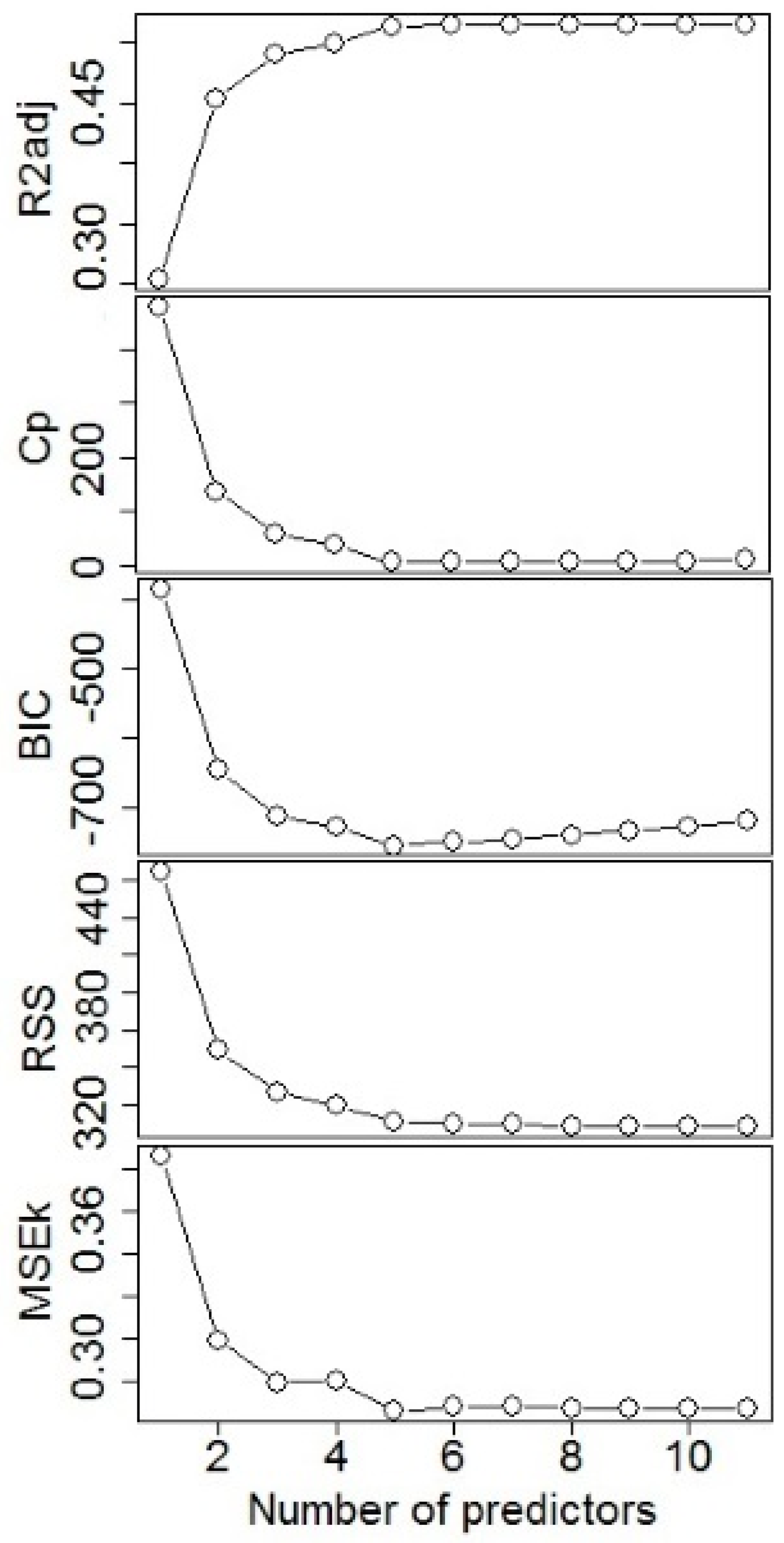
The CV regression variable selection procedure resulted in five predictors for AIDBH, that were selected according to the following goodness-of-fit statistics: R2adj, Cp, BIC, RSS, and MSEK (Figure 2). All model parameter estimates were significant with p < 0.001, and estimated parameters are presented in Table 2. The resulting expression of the model is:
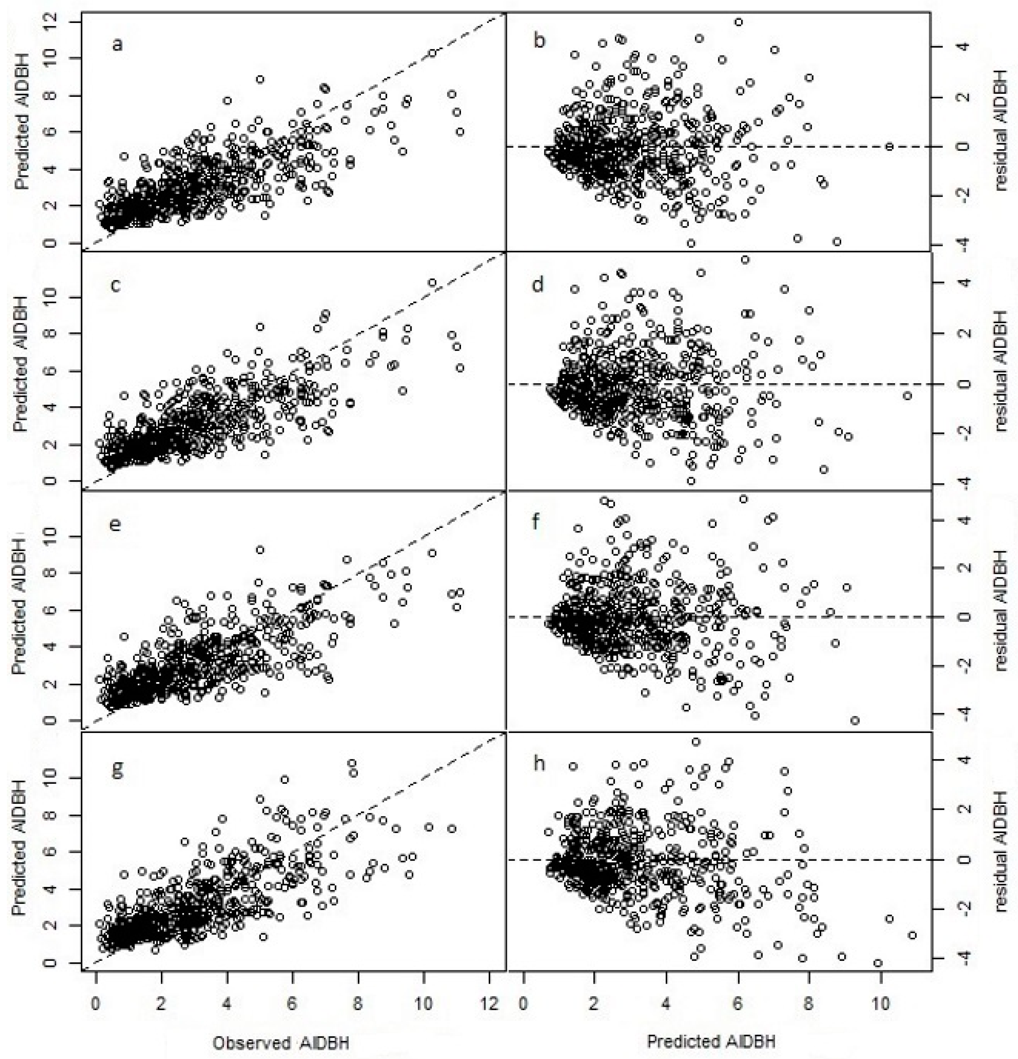
where to are parameters to estimate, e is the error term, and the other terms were previously described. The validation for the CV selection model prediction resulted in R2emp of 0.56, with a RMSE% of 44.16% and a BIAS% of −1.96% (see Table 3). Thus, the model predictions have moderate accuracy (in terms of RMSE%), but have negligible bias (Figure 3).
The model selection using LASSO regression originally had eight predictors; however, after accounting for VIF values, the final LASSO model resulted in seven predictors. The tuning parameter λ obtained by cross-validation was 5.5 × 10⁻⁴. In contrast to the CV regression model, LASSO also incorporated BALr and Ad as predictors, so the final expression of this model was:
where to are parameters to estimate (see Table 2). This model had similar goodness-of-fit statistics as the CV regression, with R2emp of 0.57, RMSE% of 44.16 and BIAS% of −2.94.
The diameter growth model was also extended to incorporate species and growth zone, specifically the CV model was fitted with these factors and their interactions with every predictor. These factors were added individually (i.e., Zone, SP) or using a combination of both terms as a unique new factor (SpZone). Interestingly, a backward selection procedure eliminated all of these interactions (p > 0.05), resulting in models that only describe different intercepts for each of the levels of these factors (Table 3). The best model included the combined factor of SpZone (CV + SpZone) as:
where αij is the intercept parameter for the ith species in the jth zone, and to are slope parameters to estimate. SpZoneij are the dummy variables associated with the ijth group specie and zone. The species were coded as: 1 (N. alpina), 2 (N. obliqua) and 3 (N. dombeyi). The other model terms were described previously. Note that with the incorporation of SpZoneij, the predictor SDI was removed from the model as it resulted not significant (p = 0.297). The goodness-of-fit statistics for this extended model were R2emp = 0.56, RMSE% = 44.49%, and BIAS% = −2.29%. This model had similar performance than the CV model (Table 4); however, from the analysis of variance, the factor SpZone resulted highly significant (p < 0.001).
Similarly, the LASSO regression model was extended by incorporating the SpZone factor (LASSSO + SpZone) and a new tuning parameter (λ = 3.9 × 10⁻³). Here, the final model obtained was:
where to are parameters to estimate, and the other terms were described previously. The goodness-of-fit statistics for this model were R2emp = 0.54, RMSE% = 45% and BIAS% = −4.31%, values that are worst in performance with respect to other three previous models evaluated (Table 4).
Note that standard errors and P-values for LASSO and LASSO + SpZone are not reported as it is not theoretically possible to obtain reliable unbiased estimates of standard errors for LASSO [35,37]. In addition, note that the 0* based on Baskerville [43] correction of CV, LASSO, CV + SpZone, and LASSO + SpZone models were 2.546, −0.160, 2.829, and −1.239, respectively.
The four predictive models of AIDBH were assessed using different DBH classes (5–15, 15–30, >30 cm) to better provide for more complete comparisons of model performance (Figure 4). For RMSE%, the CV, LASSO, and CV + SpZone models had similar performances with lower values for the intermediate class (15–30). The LASSO + SpZone model had better performance for the other two classes; however, much larger RMSE% were obtained for the intermediate class. In the case of BIAS%, all four models resulted in similar performance across all DBH classes. Overall, the best model corresponded to CV + SpZone; however, it presented larger negative BIAS% for the class >30 cm, and both of the LASSO regression models had the smallest bias for the same class.
3.2. Model Projection
Model validation results for DBH using the projection dataset were good for all models with R2emp > 0.97 (Table 5). The CV and LASSO regression had better goodness-of-fit statistics, while LASSO + SpZone had the worst performance. A six year projection for DBH showed that LASSO regression had a better R2emp of 0.99 and RMSE% of 7.26 but with marginally larger BIAS% of 0.36 than the CV model, although all models had excellent statistics. CV and LASSO regression for a simulation period of 12 years continued with good prediction performance. CV regression presented R2emp of 0.97, RMSE% of 9.66 and BIAS% of 1.75, at the same projection time, with similar results for LASSO regression with R2emp of 0.97, RMSE% of 9.50 and BIAS% of 1.96. Surprisingly, the extended models with species and growth zone factors were not clearly better than those without them.
3.3. Selected Model
The LASSO + SpZone model exhibited poor performance for both fitting and projection, with a negative bias. In contrast, the CV, LASSO, and CV + SpZone models presented similar performance in terms of goodness-of-fit statistics. However, LASSO regression had a larger bias and, in addition, included two more predictors than the CV model. Hence, the CV model could be considered the best model, but analyses of variance for CV + SpZone found that the SpZone factor was highly significant (p < 0.001). Thus, the final selected model for this study was CV + SpZone. Based on this model, incorporating species and growth zone confirms the differences concerning DBH growth from the fitting database (for comparisons between species see Table 1).
For the CV + SpZone model, the calculated least squares means indicated important differences among the levels of the combined factor SpZone (Table 6). First, these results show similar DBH growth for N. dombeyi across all RORACO growth zones. Second, N. obliqua also has a similar response in all growth zones, except for zone 3 with higher rates, and this is probably because this zone is characterized by high precipitation and long growing seasons. Third, N. alpina presented the largest differences between zones, where growth seems to increase with altitude (e.g., zone 4, Andes mountain ranges, which has the highest growth rates). Therefore, these results further justify the inclusion of the combined factor SpZone in the final selected model (CV + SpZone).
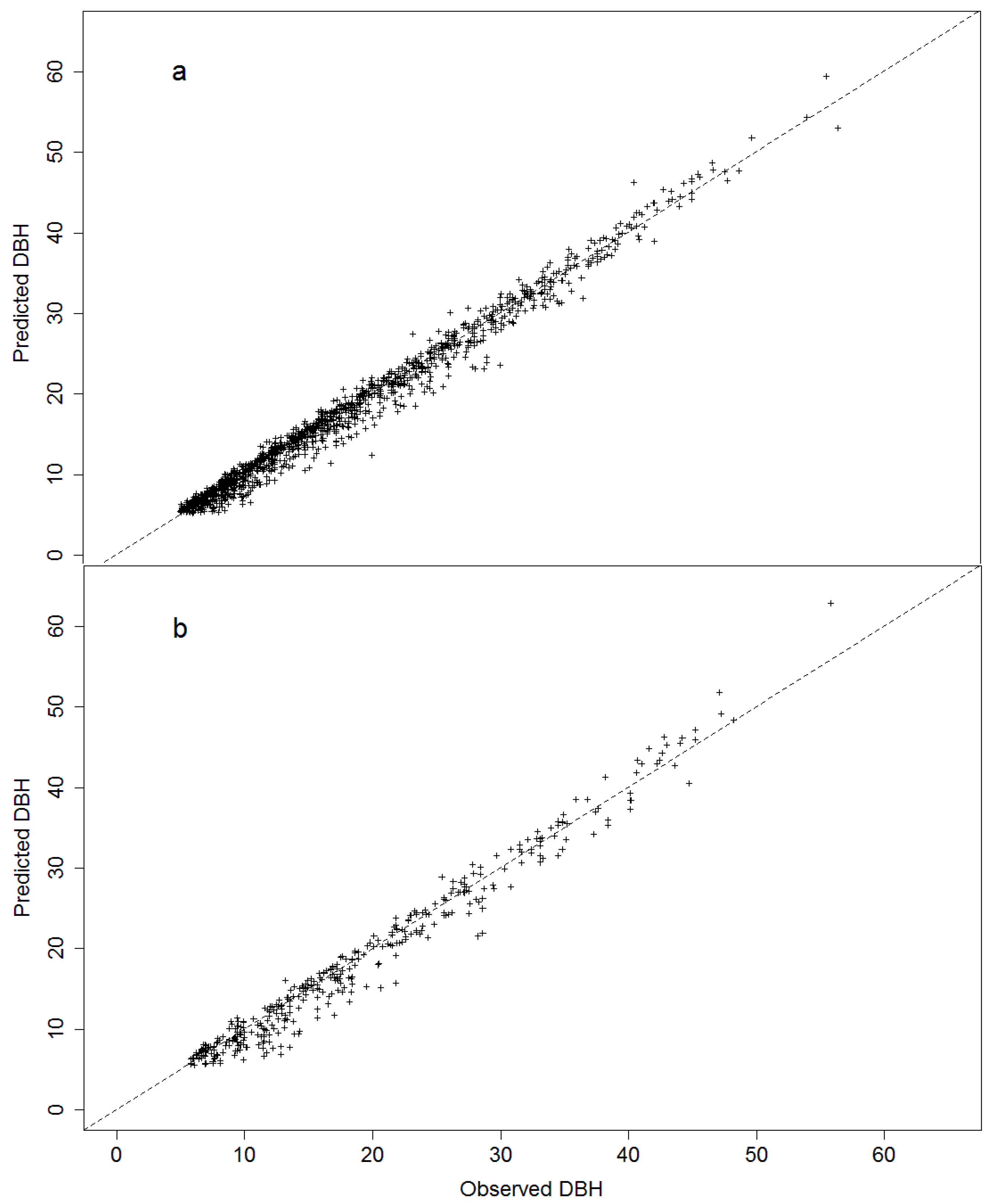
The validation using the projection dataset for the CV + SpZone model shows high predictive power for estimating future individual-tree DBH growth for a period of 6 years, and projection of up to 12 years presents consistent results (Figure 5).
4. Discussion
Diameter growth models have been recognized as useful for projecting individual-tree growth [18,19,40]. In this study, a DBH growth distance-independent model was developed for mixed Nothofagus second growth forest in southern Chile. The response variable for this study was annual average DBH growth obtained over a period of two years that originated from increment cores and tree sections. Several important aspects are associated with the use of this response variable. First, a short time period of two years was chosen to improve the association of observed tree growth with its present tree and stand conditions, a relationship that weakens as the period gets longer. This is often critical for those years with ecological disturbances (e.g., climatic, diseases, catastrophic event); however, Andreassen and Tomter [24] found no effects on the prediction accuracy with different growth period lengths. Second, no evidence of wood compression was found in increment cores when compared to sections. Finally, individual basal area growth was discarded as a response as it presented poorer goodness-of-fit statistics than DBH growth (data not shown).
Individual-tree growth models that include predictors of competition, productivity, tree- and stand-level have been used in many reported studies [21,22,23,24,25,26,27,49]. Hence, there are potentially many predictors that might describe the same biological factor, which will suffer from multicollinearity producing inconsistences and unexpected results in the fitted models [31]. Thus, it is necessary to select an adequate subset of these predictors using some variable selection procedure. In this study, the fitting database contained, as expected, pairs of predictors with high correlation, such as BA-BAN, Hd-RS, BA-SDI, BAL-BALn, Hd-QD, A-Ad, RS-QD, and DBH-H, with correlation values greater than 0.83, and this required the implementation of appropriate variable selection procedures such as CV and LASSO regression that deal with multicollinearity.
The predictors selected by CV and LASSO regression corresponded to competition, tree- and stand-level variables, but they did not included predictors associated with productivity. In CV regression DBH, A, SS, SDI, and BALn were the selected predictors, while in LASSO regression these were the same with the addition of Ad and BALr. The tree-level variables selected corresponded to DBH and A, both mostly measures of tree size; where, according to the estimated parameters, growth rates increase with larger diameters; however, age had a negative slope, indicating that at a fixed DBH value, older trees present lower growth rates. This agrees with a similar result reported by Cubillos [50] in N. alpina.
In our study, competition variables had a high relevance in explaining individual-tree growth, as found in other Nothofagus studies [50,51,52,53,54]. Interestingly, the predictor BALn (basal area of larger trees only for Nothofagus) was selected instead of BAL (that includes all species). The selection of BALn indicates that light, water and nutrients competition is related to individuals of the same cohort, in this case, the first strata of Nothofagus for one side and the companion species for the other. This ‘independence’ between these groups is mostly due to the individual strategies of each cohort, where some are shade intolerant (Nothofagus) and others shade tolerant (companion species) eliminating, or reducing, competition for light. Competition for water and nutrients is also expected to be limited as it is related to roots depth, where Nothofagus are older than the companion species using greater soil depth [2,55]. However, the fine root biomass for N. dombeyi is concentrated in the first 30 cm of depth sharing the same space that companion species, thus the no nutrients competition between this two cohorts are related to the effect of ectomycorrhizal (Nothofagus), arbuscular mycorrhizae (companion species) and fertility of this volcanic soils [55,56]. This null or limited competition between cohorts agrees with findings from previous reports that support the theory of additive effects in growth for Nothofagus and companion species [55,57,58], that translates into independent behavior (and therefore models) between these two cohorts. Lastly, productivity predictors, such as SI, were not selected for modelling DBH growth in these forests, which is probably due to several factors, such as uncertainty on the quality of dominant height-site models, and measurement errors on dominant height and age, among others.
The average DBH growth rates for combinations of species and zone varied considerably, with important differences between species and zone; however, extreme cases where noted for the group combinations of N. alpine—zone 1, and N. dombeyi—zone 3, with an 88% larger growth rate for the latter (2.15 mm year−1 against 4.05 mm year−1). Other studies also have found contrasting differences in growth between Nothofagus species and growth zones [5,9,10,59,60,61,62,63,64]. The incorporation of species and/or zone factors to improve growth models has been previously reported [24,25]. In the present study, the combined specie-zone factor (SpZone, with 11 levels), explained more variability than the individual two factors (with seven levels for both species and zone), indicating that a greater disaggregation of the data is required to model growth rate accurately. Interestingly, the LASSO + SpZone model selected as predictors for the combined factor SpZone the extreme groups (Table 6), by combining the central five levels into a single group class.
The fitting of the four candidate models to predict AIDBH resulted in overall good performance, with R2emp ranging from 0.54 to 0.57, RMSE% of ~44%, and a BIAS% smaller than 3%. Similar goodness-of-fit statistics have been reported in other species for AIDBH models with R2emp ranging from 0.26 to 0.68 [24,26,51,65]. AIDBH projections for 6 and 12 years resulted in R2emp ranges of 0.23–0.28 and 0.15–0.24, respectively. This drop in performance is likely to have been affected by the quality of the projection database, that included, for example, 6 years with 20% of the trees with null or negative DBH increments, probably due to field measurement errors and low growth rates for these species. In contrast, for both Nothofagus and companion species, DBH projections for 6 and 12 years resulted in overall R2emp values greater than 0.97. Small diameter trees (DBH < 15 cm) presented lower correlations, with values of 0.88 and 0.58 for projections of 6 and 12 years, respectively. In addition, as expected, goodness-of-fit statistics were better for the Nothofagus cohort than the companion species cohort.
The final selected model in this study is CV + SpZone (Equation (10)). The LASSO model was discarded, even though it was highly competitive, due to lower prediction performance, and it also included some predictors with high multicollinearity (VIF > 5). LASSO + SpZone had the worst performance with issues for prediction and projection. The CV model presented better goodness-of-fit statistics than the CV + SpZone model; however, the combined factor SpZone was highly significant (p < 0.001). Hence, the inclusion of SpZone is strongly justified given the wide geographical range of this population and its differential diameter growth responses. This large stand variability has also been detected before, leading to many authors defining growth zones for this resource [9,10,11]. Alternatively, with no information of growth zone, it is possible to use the simple CV model that will still provide reliable predictions of AIDBH.
The simplified final selected model corroborates well known forest ecological processes and basic biological consistency in the parameter estimates (Table 2). For example, BALn and SS are competition variables where a higher value indicates a high competition for a given tree, and their model parameters both have a negative sign; hence, with higher competition there are lower growth rates. In the case of the inverse of BALr, the estimated coefficient value is positive, thus a high competition produces a lower growth rate, and vice versa. The most important predictor, DBH, has a strong effect on growth, where larger trees have a greater diameter increment due to its positive sign, which is expected as this effect is controlled indirectly by age. Hence, at the same age, larger trees tend to have greater growth rates. Finally, the parameter associated with age was negative, thus for a fixed DBH value, a young tree is capable of higher growth rates than an older tree.
The advantages of CV procedure as a selection method is the possibility of obtaining an independent estimation of the mean square error (MSEK) when compared to other stepwise methods. LASSO is an alternative procedure that regularizes the coefficient estimates, forcing some of them to be exactly equal to zero, and hence, performing variable selection. Both procedures, CV and LASSO, have been used broadly due their advantages to identify those variables that help to better predict a given response [32]. Similarly, the importance of incorporating dummy variables (or factors) in a linear model helps to expand model specificity, where additional factors can modify intercepts or slopes from the original regression model to make obtain more generic, and therefore robust, models that apply for wider conditions.
The final reported model should be used within the temporal and spatial frame of inference for RORACO second growth forests located between 37° and 41.5° south latitude, with breast height ages ranging from 20 to 80 years, and with a Nothofagus basal area greater than 60% of the total basal area, due to the characteristics of the database used in this study (Table 1). Similarly, it is recommended that this model is used for projections no longer than 12 years. For this projection period, the temporal frame of inference for this model is well suited for existing forest management plans in Chile that typically consider durations of 10 years, among a range of silvicultural interventions.
Future research is warranted to better improve the performance of models of individual-tree growth for this population. Some of these extensions could include: (1) producing models that do not require age, as this predictor is often difficult to obtain from typical forest inventories for natural stands; (2) including extra validation data from a wider geographic range and with additional forest conditions; (3) developing an individual-tree growth model for companion species; (4) implementing a fully individual-tree model routine that includes a mortality and a height growth module; and (5) developing a compatible system based on both individual-tree and stand-level models.
5. Conclusions
A comparison of two selection predictor procedures to estimate individual-tree annual increment in DBH was presented using data from a mixed second growth forest conformed by N. alpina, N. obliqua, and N. dombeyi in southern Chile. This study selected a model based on a small set of predictors that successfully explained a large portion of the variability of annual DBH growth, with variables associated with competition, tree- and stand-level components; however, no variables associated with site productivity were selected. The results of this study indicate that a model that uses a cross-validation procedure with the incorporation of a combined factor for specie and zone (CV + SpZone) is sufficient and provides a simple and valuable tool to support management decisions for this important ecosystem in southern Chile.
Acknowledgments
This research was supported by the University of Florida through the School of Forest Resources & Conservation. The authors acknowledge Alicia Ortega and Guillermo Trincado from the Universidad Austral de Chile for facilitating the two Nothofagus plot datasets.
Author Contributions
P.C.M. and S.P. built the different databases; P.C.M. and S.A.G. conceived and fitted the models; P.C.M. and S.A.G. wrote the paper, with significant contributions from W.P.C, F.J.E. and S.P.
Conflicts of Interest
The authors declare no conflict of interest.
References
- Donoso, C. Variación natural en especies de Nothofagus en Chile. Bosque 1987, 8, 85–97. Available online: http://mingaonline.uach.cl/pdf/bosque/v8n2/art03.pdf (accessed on 15 July 2017). [CrossRef]
- Donoso, C. Bosques Templados de Chile y Argentina: Variación, Estructura y Dinámica; Editorial Universitaria: Santiago, Chile, 1993. [Google Scholar]
- Corporación Nacional Forestal (CONAF). Catastro de los Recursos Vegetacionales Nativos de Chile. Monitoreo de Cambios y Actualizaciones. Periodo 1997–2011; Ministerio de Agricultura: Santiago, Chile, 2011.
- Instituto Forestal (INFOR). Bosque nativo 12; Ministerio de Agricultura: Santiago, Chile, 2016.
- Donoso, C.; Premoli, A.; Gallo, L.; Ipinza, R. Variación Intraespecífica en las Especies Arbóreas de los Bosques Templados de Chile y Argentina; Editorial Universitaria: Santiago, Chile, 2004. [Google Scholar]
- Gezan, S.A.; Ortega, A.; Andenmatten, E. Diagramas de manejo de densidad para renovales de roble, raulí y coigüe en Chile. Bosque 2007, 28, 97–105. [Google Scholar] [CrossRef]
- Moreno, P.C. Individual-Tree Diameter Growth Models and Variability of Mixed Nothofagus Second Growth Forests in Southern Chile. Master’s Thesis, University of Florida, Gainesville, FL, USA, 2017. [Google Scholar]
- Instituto Forestal (INFOR). Rentabilidad Económica de Distintas Propuestas Silvícolas para Renovales de Nothofagus en el Centro sur de Chile. Informe Técnico 193; Ministerio de Agricultura: Santiago, Chile, 2013.
- Echeverrıa, C.; Lara, A. Growth patterns of secondary Nothofagus oblique—N. alpina forests in southern Chile. For. Ecol. Manag. 2004, 195, 29–43. [Google Scholar] [CrossRef]
- Donoso, P.; Donoso, C.; Sandoval, V. Proposición de zonas de crecimiento de renovales de roble (Nothofagus obliqua) y raulí (Nothofagus alpina) en su rango de distribución natural. Bosque 1993, 14, 37–55. Available online: http://mingaonline.uach.cl/pdf/bosque/v14n2/art06.pdf (accessed on 19 July 2017). [CrossRef]
- Gezan, S.A.; Moreno, P.C. Establecimiento y medición de una red de parcelas permanentes para renovales de roble (Nothofagus obliqua), raulí (Nothofagus alpina) y coigüe (Nothofagus dombeyi). Bosque Nativo. 1999, 22, 9–11. [Google Scholar]
- Shortt, J.S.; Burkhart, H.E. A comparison of loblolly pine plantation growth and yield models for inventory updating. South J. Appl. For. 1996, 20, 15–22. [Google Scholar]
- Moreno, P.C. Proposición Preliminar de Curvas de Índice de Sitio para Renovales de Raulí. Ph.D. Thesis, Universidad de Chile, Santiago, Chile, 2001. [Google Scholar]
- Salas, C.; García, O. Modelling height development of mature Nothofagus obliqua. For. Ecol. Manag. 2006, 229, 1–6. [Google Scholar] [CrossRef]
- Ugalde, G.A. Crecimiento en Altura de Renovales de Lenga (Nothofagus pumilio (Poepp. et endl.) Krasser) en Monte alto (XII región) en Función de la Calidad del Sitio. Ph.D. Thesis, Universidad de Chile, Santiago, Chile, 2006. [Google Scholar]
- Birdsey, R. Updating Methods for Forest Inventories: An Overview; USDA Forest Service General Technical Report; PNW-GTR-Pacific Northwest Research Station: Washington, DC, USA, 1990. [Google Scholar]
- Blanco, J.A.; González de Andrés, E.; San Emeterio, L.; Lo, Y.H. Modelling mixed forest stands: Methodological challenges and approaches. In Advanced Modelling Techniques Studying Global Changes in Environmental Sciences; Lek, S., Park, Y.S., Baehr, C., Jorgensen, S.E., Eds.; Elsevier: Amsterdam, The Netherlands, 2015; pp. 187–213. [Google Scholar]
- Burkhart, H.E.; Tomé, M. Modeling Forest Trees and Stands; Springer: Dordrecht, The Netherlands, 2012. [Google Scholar]
- Vanclay, J.K. Modelling Forest Growth and Yield: Applications to Mixed Tropical Forests; CAB International: Wallingford, UK, 1994. [Google Scholar]
- Gonzalez-Benecke, C.A.; Gezan, S.A.; Leduc, D.J.; Martin, T.A.; Cropper, W.P.; Samuelson, L.J. Modeling survival, yield, volume partitioning and their response to thinning for longleaf pine plantations. Forests 2012, 3, 1104–1132. [Google Scholar] [CrossRef]
- Harrison, W.C.; Burk, T.E.; Beck, D.E. Individual tree basal area increment and total height equations for Appalachian mixed hardwoods after thinning. South. J. Appl. For. 1986, 10, 99–104. [Google Scholar]
- Murphy, P.A.; Graney, D.L. Individual-tree basal area growth, survival, and total height models for upland hardwoods in the Boston mountains of Arkansas. South. J. Appl. For. 1998, 22, 184–192. [Google Scholar]
- Huang, S.; Titus, S.J. Estimating a system of nonlinear simultaneous individual tree models for white spruce in boreal mixed-species stands. Can. J. For. Res. 1999, 29, 1805–1811. [Google Scholar] [CrossRef]
- Andreassen, K.; Tomter, S.M. Basal area growth models for individual trees of norway spruce, scots pine, birch and other broadleaves in Norway. For. Ecol. Manag. 2003, 180, 11–24. [Google Scholar] [CrossRef]
- Pukkala, T.; Lähde, E.; Laiho, O. Growth and yield models for uneven-sized forest stands in Finland. For. Ecol. Manag. 2009, 258, 207–216. [Google Scholar] [CrossRef]
- Nunes, L.; Tomé, J.; Tomé, M. Prediction of annual tree growth and survival for thinned and unthinned even-aged maritime pine stands in Portugal from data with different time measurement intervals. For. Ecol. Manag. 2011, 262, 1491–1499. [Google Scholar] [CrossRef]
- Ma, W.; Lei, X. Nonlinear simultaneous equations for individual-tree diameter growth and mortality model of natural mongolian oak forests in northeast China. Forests 2015, 6, 2261–2280. [Google Scholar] [CrossRef]
- Burkhart, H.E. Suggestions for choosing an appropriate level for modelling forest stands. In Modelling Forest Systems; Amaro, A., Reed, D., Soares, P., Eds.; CAB International: Wallingford, UK, 2003; pp. 3–10. [Google Scholar]
- Buckman, R.E. Growth and Yield of Red Pine in Minnesota; Technical Bulletin 1272; US Department of Agriculture: Washington, DC, USA, 1962.
- Huang, S.; Titus, S.J. An individual tree diameter increment model for white spruce in Alberta. Can. J. For. Res. 1995, 25, 1455–1465. [Google Scholar] [CrossRef]
- Welham, S.J.; Gezan, S.A.; Clark, S.; Mead, A. Statistical Methods in Biology: Design and Analysis of Experiments and Regression; CRC Press: Boca Raton, FL, USA, 2014. [Google Scholar]
- James, G.; Witten, D.; Hastie, T.; Tibshirani, R. An Introduction to Statistical Learning; Springer: New York, NY, USA, 2013. [Google Scholar]
- Hastie, T.; Tibshirani, R.; Friedman, J. The Elements of Statistical Learning: Data Mining, Inference, and Prediction; Springer: New York, NY, USA, 2009. [Google Scholar]
- Tibshirani, R. Regression shrinkage and selection via the lasso. J. R. Stat. Soc. B. 1996, 58, 267–288. Available online: http://www.jstor.org/stable/2346178 (accessed on 5 July 2017).
- Kyung, M.; Gill, J.; Ghosh, M.; Casella, G. Penalized regression, standard errors, and bayesian lassos. Bayesian Anal. 2010, 5, 369–411. [Google Scholar] [CrossRef]
- Wu, T.T.; Chen, Y.F.; Hastie, T.; Sobel, E.; Lange, K. Genome-wide association analysis by lasso penalized logistic regression. Bioinformatics 2009, 25, 714–721. [Google Scholar] [CrossRef] [PubMed]
- Lockhart, R.; Taylor, J.; Tibshirani, R.J.; Tibshirani, R. A significance test for the lasso. Ann. Stat. 2014, 42, 413–468. [Google Scholar] [CrossRef] [PubMed]
- Ortega, A.; Gezan, S.A. Cuantificación de crecimiento y proyección de calidad en Nothofagus. Bosque 1998, 19, 123–126. Available online: http://mingaonline.uach.cl/scielo.php?pid=S0717-92001998000100013&script=sci_arttext&tlng=es (accessed on 25 July 2017). [CrossRef]
- Corporación Nacional Forestal (CONAF); Comisión Nacional del Medio Ambiente (CONAMA); Banco Internacional de Reconstrucción y Fomento (BIRF); Universidad Austral de Chile; Pontificia Universidad Católica de Chile; Universidad Católica de Temuco. Proyecto Catastro y Evaluación de los Recursos Vegetacionales Nativos de Chile; Ministerio de Agricultura: Santiago, Chile, 1999.
- Avery, T.E.; Burkhart, H. Forest Measurements, 5th ed.; McGraw-Hill: New York, NY, USA, 2002. [Google Scholar]
- Pukkala, T.; Lähde, E.; Laiho, O. Using optimization for fitting individual-tree growth models for uneven-aged stands. Eur. J. For. Res. 2011, 130, 829–839. [Google Scholar] [CrossRef]
- Lumley, T.; Miller, A. Leaps: Regression Subset Selection. R Package Version 3.0. 2017. Available online: https://cran.r-project.org/web/packages/leaps/index.html (accessed on 5 July 2017).
- Baskerville, G. Use of logarithmic regression in the estimation of plant biomass. Can. J. For. Res. 1972, 2, 49–53. [Google Scholar] [CrossRef]
- Ahlburg, D.A. Forecast evaluation and improvement using theil’s decomposition. J. Forecast. 1984, 3, 345–351. [Google Scholar] [CrossRef]
- Blanco, J.A.; Seely, B.; Welham, C.; Kimmins, J.; Seebacher, T.M. Testing the performance of a forest ecosystem model (forecast) against 29 years of field data in a pseudotsuga menziesii plantation. Can. J. For. Res. 2007, 37, 1808–1820. [Google Scholar] [CrossRef]
- Fox, J.; Monette, G. Generalized collinearity diagnostics. J. Am. Stat. Assoc. 1992, 87, 178–183. [Google Scholar] [CrossRef]
- R Development Core Team. R: A Language and Environment for Statistical Computing; R Foundation for Statistical Computing: Vienna, Austria, 2015; Available online: http://www.r-project.org (accessed on 3 January 2017).
- Friedman, J.; Hastie, T.; Simon, N.; Tibshirani, R. Glmnet: Lasso and Elastic-Net Regularized Generalized Linear Models. R Package Version 1.9-5; R Foundation for Statistical Computing: Vienna, Austria, 2016. [Google Scholar]
- Peng, C. Growth and yield models for uneven-aged stands: Past, present and future. For. Ecol. Manage. 2000, 132, 259–279. Available online: http://flash.lakeheadu.ca/~chpeng/reprint_uneven-age.pdf (accessed on 9 July 2017). [CrossRef]
- Cubillos, D. Modelos de crecimiento diametral para algunos renovales de raulí. Cienc. Investig. For. 1987, 1, 67–76. [Google Scholar]
- Monserud, R.A.; Sterba, H. A basal area increment model for individual trees growing in even-and uneven-aged forest stands in Austria. For. Ecol. Manag. 1996, 80, 57–80. [Google Scholar] [CrossRef]
- Coomes, D.A.; Allen, R.B. Effects of size, competition and altitude on tree growth. J. Ecol. 2007, 95, 1084–1097. [Google Scholar] [CrossRef]
- Richardson, S.J.; Hurst, J.M.; Easdale, T.A.; Wiser, S.K.; Griffiths, A.D.; Allen, R.B. Diameter growth rates of beech (Nothofagus) trees around New Zealand. N. Z. J. For. 2011, 56, 3–11. Available online: http://nzjf.org.nz/free_issues/NZJF56_1_2011/9B1010A2-B122-4805-9290-E4144A6738D1.pdf (accessed on 18 July 2017).
- Ivancich, H.S.; Martínez Pastur, G.J.; Lencinas, M.V.; Cellini, J.M.; Peri, P.L. Proposals for Nothofagus antarctica diameter growth estimation: Simple vs. Global models. J. For. Sci. 2014, 60, 307–317. Available online: http://ri.conicet.gov.ar/bitstream/handle/11336/5497/CONICET_Digital_Nro.6975_D.pdf?sequence=5&isAllowed=y (accessed on 1 July 2017).
- Lusk, C.H.; Ortega, A. Vertical structure and basal area development in second-growth Nothofagus stands in Chile. J. Appl. Ecol. 2003, 40, 639–645. [Google Scholar] [CrossRef]
- Moreno-Chacón, M.; Lusk, C.H. Vertical distribution of fine root biomass of emergent Nothofagus dombeyi and its canopy associates in a Chilean temperate rainforest. For. Ecol. Manag. 2004, 199, 177–181. [Google Scholar] [CrossRef]
- Donoso, P.J.; Lusk, C.H. Differential effects of emergent Nothofagus dombeyi on growth and basal area of canopy species in an old-growth temperate rainforest. J. Veg. Sci. 2007, 18, 675–684. [Google Scholar] [CrossRef]
- Donoso, P.J.; Soto, D.P. Does site quality affect the additive basal area phenomenon? Results from Chilean old-growth temperate rainforests. Can. J. For. Res. 2016, 46, 1330–1336. [Google Scholar] [CrossRef]
- Schlatter, J.; Gerding, V.; Adriazola, J. Sistema de Ordenamiento de la Tierra. Herramienta para la Planificación Forestal, Aplicada a las Regiones VII, VIII y IX; Serie Técnica; Facultad Ciencias Forestales, Universidad Austral de Chile: Valdivia, Chile, 1994. [Google Scholar]
- Schlatter, J.; Gerding, V.; Adriazola, J. Sistema de Ordenamiento de la Tierra. Herramienta para la Planificación Forestal, Aplicada para la X Región; Serie técnica; Facultad Ciencias Forestales, Universidad Austral de Chile: Valdivia, Chile, 1995. [Google Scholar]
- Chauchard, L.; Sbrancia, R. Modelos de crecimiento diamétrico para Nothofagus obliqua. Bosque 2003, 24, 3–16. [Google Scholar] [CrossRef]
- Thiers, O.; Gerding, V.; Hildebrand, E. Renovales de Nothofagus obliqua en centro y sur de Chile: Factores de sitio relevantes para su productividad. In Libro de Actas de eco Reuniones. Segunda Reunión Sobre los Nothofagus en la Patagonia; Bava, J., Picco, O., Pildaín, M., López, P., Orellana, I., Eds.; Centro de Investigación y Extensión Forestal Andino Patagónico (CIEFAP): Esquel, Argentina, 2008; pp. 255–260. [Google Scholar]
- Gezan, S.A.; Moreno, P.; Ortega, A. Modelos fustales para renovales de roble, raulí y coigüe en Chile. Bosque 2009, 30, 61–69. [Google Scholar] [CrossRef]
- Esse, C.; Donoso, P.J.; Gerding, V.; Encina-Montoya, F. Determination of homogeneous edaphoclimatic zones for the secondary forests of Nothofagus dombeyi in central-southern chile. Cienc. Investig. Agrar. 2013, 40, 351–360. [Google Scholar] [CrossRef]
- Wykoff, W.R. A basal area increment model for individual conifers in the northern Rocky Mountains. For. Sci. 1990, 36, 1077–1104. [Google Scholar]
Figure 1.
Geographical localization of permanent plots (PP) and temporary plots (TP) networks. Growth zones defined by Gezan and Moreno [11] are also shown.
Figure 1.
Geographical localization of permanent plots (PP) and temporary plots (TP) networks. Growth zones defined by Gezan and Moreno [11] are also shown.
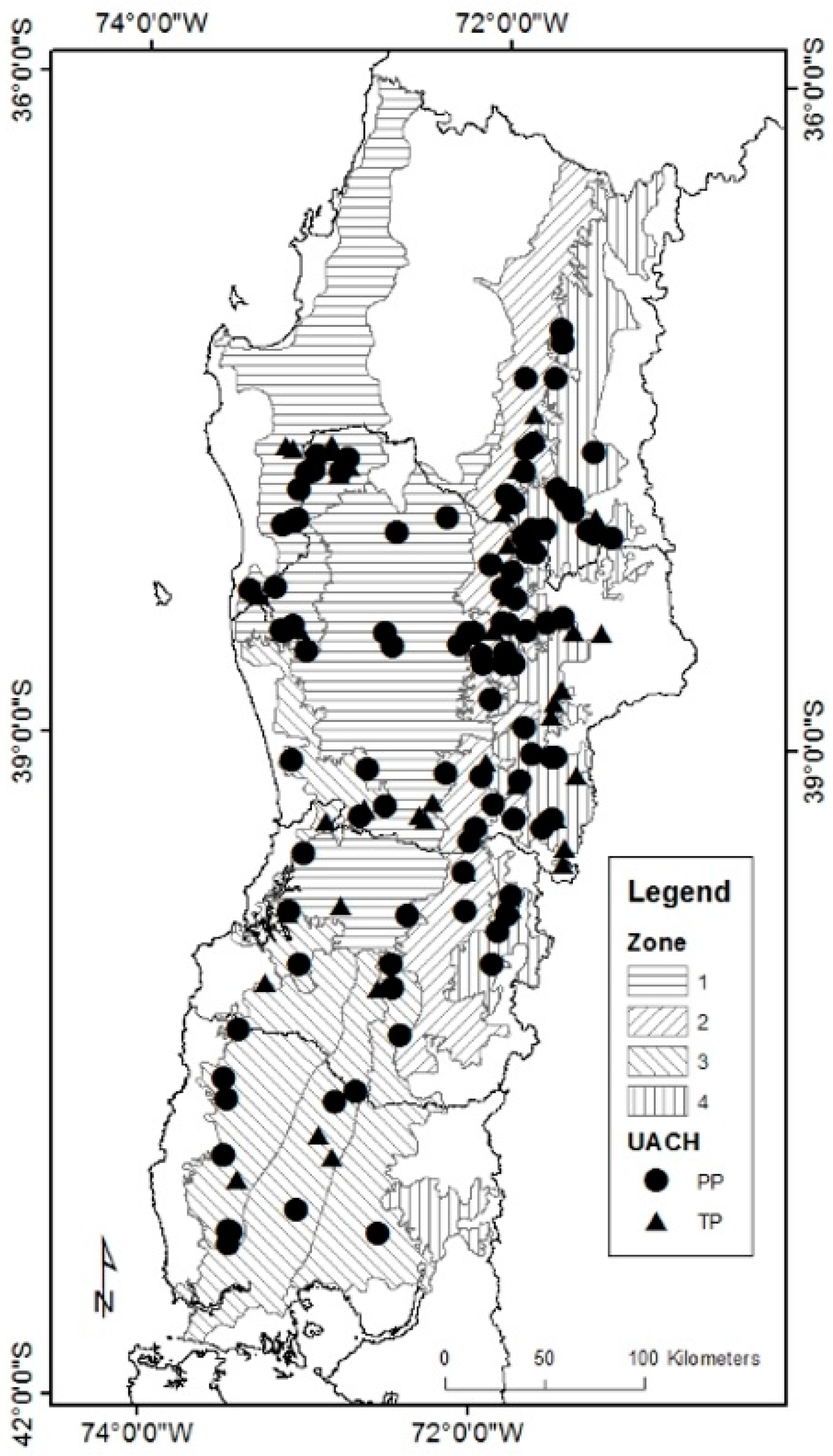
Figure 2.
Goodness-of-fit statistics of adjusted r-squared (R2adj), Statistics Mallows’ Cp, Schwartz’s information criterion (BIC), residual sum of squares (RSS), and the mean squared error averaged over the K folds (MSEK) for different number of predictors with cross-validation (CV) regression selection model using the fitting database.

Figure 3.
Fit and residuals plots for the natural logarithm of annual increment in diameter at breast height (AIDBH, mm year−1) of selected models using test dataset. Cross-validation (CV, (a,b)); LASSO (c,d); cross-validation with specie-zone factor (CV + SpZone, (e,f)); and LASSO with specie-zone factor (LASSO + SpZone, (g,h)).

Figure 4.
Relative root mean square error (RMSE%, (a)) and relative bias (BIAS%, (b)) calculated by DBH classes for selected models using the test dataset.
Figure 4.
Relative root mean square error (RMSE%, (a)) and relative bias (BIAS%, (b)) calculated by DBH classes for selected models using the test dataset.
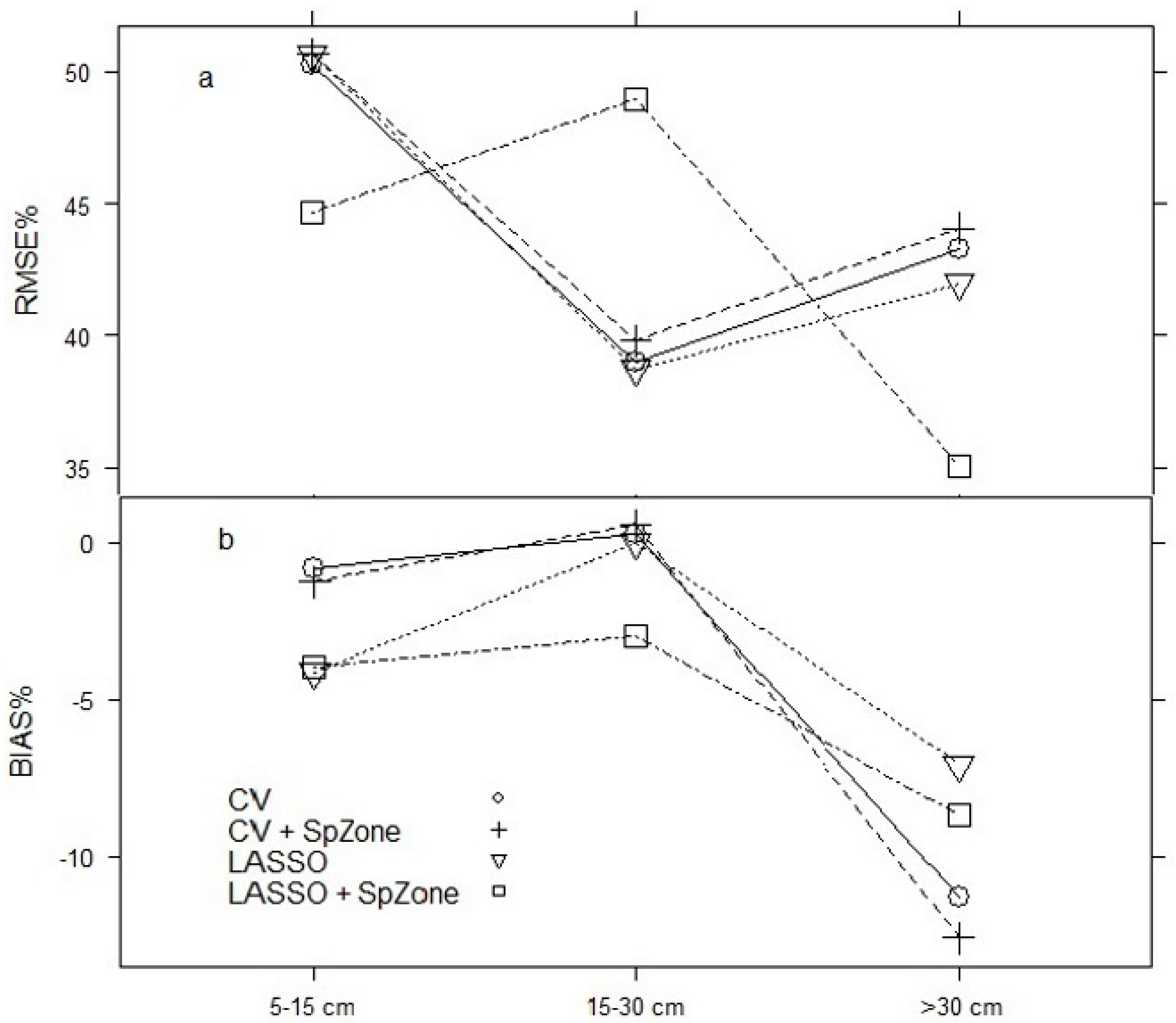
Figure 5.
Projection for diameter at breast height (cm) using a period of 6 years (2000 to 2006) (a) and 12 years (2000 to 2012) (b), using the projection database for the CV + SpZone (cross validation with species-zone factor) model. For further details and goodness-of-fit statistics see Table 5.
Figure 5.
Projection for diameter at breast height (cm) using a period of 6 years (2000 to 2006) (a) and 12 years (2000 to 2012) (b), using the projection database for the CV + SpZone (cross validation with species-zone factor) model. For further details and goodness-of-fit statistics see Table 5.


Table 1.
Summary statistics of Nothofagus spp. individual and stand attributes for fitting database based on data from the permanent plots (PP) and temporary plots (TP) network.
Table 1.
Summary statistics of Nothofagus spp. individual and stand attributes for fitting database based on data from the permanent plots (PP) and temporary plots (TP) network.
| Tree Species | Nothofagus alpina | Nothofagus obliqua | Nothofagus dombeyi | ||||||||||||
| Tree Variables | n | Mean | SD | Min | Max | n | Mean | SD | Min | Max | n | Mean | SD | Min | Max |
| DBH | 202 | 16.7 | 9.8 | 5.0 | 42.7 | 627 | 17.0 | 10.0 | 5.0 | 62.1 | 279 | 19.3 | 11.3 | 5.0 | 60.2 |
| H | 202 | 15.2 | 6.6 | 4.2 | 34.5 | 627 | 16.1 | 7.3 | 3.5 | 45.0 | 279 | 16.2 | 6.1 | 4.2 | 34.5 |
| A | 202 | 36.7 | 14.2 | 11.0 | 104.0 | 627 | 30.6 | 14.6 | 8.0 | 95.0 | 279 | 32.5 | 13.2 | 9.0 | 80.0 |
| BAL | 202 | 26.0 | 16.8 | 0.0 | 83.4 | 627 | 19.0 | 14.0 | 0.0 | 65.1 | 279 | 28.0 | 20.6 | 0.0 | 92.4 |
| BALn | 202 | 20.9 | 15.0 | 0.0 | 82.3 | 627 | 15.7 | 12.3 | 0.0 | 54.9 | 279 | 20.6 | 16.6 | 0.0 | 82.2 |
| SS | 202 | 2.3 | 1.1 | 1.0 | 4.0 | 627 | 2.3 | 1.0 | 1.0 | 4.0 | 279 | 2.2 | 1.0 | 1.0 | 4.0 |
| BALr | 202 | 0.6 | 0.3 | 0.0 | 1.0 | 627 | 0.6 | 0.3 | 0.0 | 1.0 | 279 | 0.6 | 0.3 | 0.0 | 1.0 |
| AIDBH | 202 | 2.6 | 1.6 | 0.2 | 7.7 | 627 | 3.0 | 2.1 | 0.2 | 12.1 | 279 | 3.6 | 2.2 | 0.1 | 10.2 |
| Dominant Specie | Nothofagus alpina | Nothofagus obliqua | Nothofagus dombeyi | ||||||||||||
| Stand Variables | n | Mean | SD | Min | Max | n | Mean | SD | Min | Max | n | Mean | SD | Min | Max |
| BA | 24 | 46.7 | 13.8 | 10.8 | 72.3 | 87 | 35.7 | 13.0 | 9.5 | 71.5 | 47 | 55.2 | 17.8 | 23.4 | 98.4 |
| N | 24 | 2564 | 1184 | 320 | 5000 | 87 | 2378 | 1119 | 320 | 4640 | 47 | 2900 | 1357 | 880 | 5600 |
| QD | 24 | 16.4 | 4.8 | 8.5 | 30.5 | 87 | 15.4 | 6.2 | 6.8 | 33.3 | 47 | 16.9 | 5.4 | 8.4 | 30.4 |
| Hd | 24 | 21.2 | 5.7 | 10.2 | 35.1 | 87 | 20.8 | 7.0 | 7.8 | 42.4 | 47 | 20.8 | 5.9 | 9.9 | 34.1 |
| Ad | 24 | 47.5 | 10.9 | 23.0 | 77.0 | 87 | 36.6 | 14.7 | 12.7 | 86.8 | 47 | 40.2 | 13.1 | 21.3 | 85.1 |
| SI | 24 | 10.3 | 3.9 | 4.1 | 24.3 | 87 | 12.5 | 3.9 | 2.0 | 22.9 | 47 | 11.4 | 3.4 | 3.9 | 18.4 |
| BAN | 24 | 37.6 | 12.4 | 10.8 | 59.7 | 87 | 30.4 | 11.5 | 8.8 | 57.8 | 47 | 46.5 | 18.7 | 8.0 | 89.6 |
| SDI | 24 | 1212 | 336 | 406 | 1944 | 87 | 956 | 258 | 410 | 1674 | 47 | 1400 | 361 | 640 | 2305 |
| RS | 24 | 0.1 | 0.0 | 0.1 | 0.2 | 87 | 0.1 | 0.0 | 0.1 | 0.3 | 47 | 0.1 | 0.0 | 0.1 | 0.2 |
Note: n, number of observations; SD, standard deviation; min, minimum; max, maximum; DBH, diameter breast height (cm); H, total height (m); A, breast height age (years); BAL, basal area of larger trees (m2 ha−1); BALn, basal area of larger trees for Nothofagus (m2 ha−1); SS, sociological status; BALr, relative BAL; AIDBH, annual increment in DBH (mm year−1); BA, stand basal area (m2 ha−1); N, number of trees (trees ha−1); QD, quadratic diameter (cm); Hd, dominant height (m); Ad, dominant breast height stand age (years); SI, site index (m); BAN, basal area of Nothofagus (m2 ha−1); SDI, stand density index (trees ha−1); RS, relative spacing.
Table 2.
Parameter estimates of selected models for estimation of the logarithm of annual increment in diameter at breast height (AIDBH, mm year−1) for cross-validation (CV) and least absolute shrinkage and selection operator (LASSO) procedures.
Table 2.
Parameter estimates of selected models for estimation of the logarithm of annual increment in diameter at breast height (AIDBH, mm year−1) for cross-validation (CV) and least absolute shrinkage and selection operator (LASSO) procedures.
| Parameter | Estimate | SE | p-Value | VIF* | Parameter | Estimate | VIF* |
|---|---|---|---|---|---|---|---|
| CV (Equation (8)) | LASSO (Equation (9)) | ||||||
| 2.410 × 100 | 2.173 × 10⁻¹ | <0.001 | - | −3.098 × 10⁻¹ | - | ||
| −7.062 × 10⁻³ | 2.064 × 10⁻³ | <0.001 | 1.74 | −7.255 × 10⁻³ | 3.20 | ||
| 2.745 × 10⁻⁴ | 6.787 × 10⁻⁵ | <0.001 | 1.22 | 2.215 × 10⁻⁴ | 1.40 | ||
| 9.046 × 10⁻¹ | 6.798 × 10⁻² | <0.001 | 3.29 | 7.892 × 10⁻¹ | 5.28 | ||
| −1.138 × 100 | 7.488 × 10⁻² | <0.001 | 2.26 | −1.073 × 100 | 6.73 | ||
| −1.336 × 10⁻¹ | 3.149 × 10⁻² | <0.001 | 2.22 | −1.325 × 10⁻¹ | 2.44 | ||
| - | - | - | - | −4.318 × 10⁻² | 5.36 | ||
| - | - | - | - | 9.792 × 100 | 6.59 | ||
| CV + SpZone (Equation (10)) | LASSO + SpZone (Equation (11)) | ||||||
| 2.702 × 100 | 2.562 × 10⁻¹ | <0.001 | 2.09 | −1.387 × 100 | - | ||
| 2.908 × 100 | 2.345 × 10⁻¹ | <0.001 | 2.09 | 6.790 × 10⁻² | 2.28 | ||
| 3.065 × 100 | 2.397 × 10⁻¹ | <0.001 | 2.09 | −2.507 × 10⁻¹ | 2.28 | ||
| 2.538 × 100 | 2.120 × 10⁻¹ | <0.001 | 2.09 | −1.702 × 10⁻¹ | 2.28 | ||
| 2.587 × 100 | 2.219 × 10⁻¹ | <0.001 | 2.09 | −1.955 × 10⁻¹ | 2.28 | ||
| 2.841 × 100 | 2.272 × 10⁻¹ | <0.001 | 2.09 | 3.455 × 10⁻² | 2.28 | ||
| 2.678 × 100 | 2.329 × 10⁻¹ | <0.001 | 2.09 | 5.922 × 10⁻² | 2.28 | ||
| 2.946 × 100 | 2.298 × 10⁻¹ | <0.001 | 2.09 | −7.117 × 10⁻³ | 3.30 | ||
| 2.948 × 100 | 2.680 × 10⁻¹ | <0.001 | 2.09 | 8.700 × 10⁻⁵ | 2.07 | ||
| 2.941 × 100 | 2.353 × 10⁻¹ | <0.001 | 2.09 | 7.699 × 10⁻¹ | 6.21 | ||
| 2.902 × 100 | 2.358 × 10⁻¹ | <0.001 | 2.09 | −1.096 × 100 | 7.30 | ||
| −6.517 × 10⁻³ | 2.002 × 10⁻³ | 0.0012 | 1.82 | −1.293 × 10⁻¹ | 2.53 | ||
| 9.307 × 10⁻¹ | 6.970 × 10⁻² | <0.001 | 3.82 | −2.250 × 10⁻² | 5.56 | ||
| −1.175 × 100 | 7.797 × 10⁻² | <0.001 | 2.61 | 1.419 × 10⁻¹ | 6.91 | ||
| −1.401 × 10⁻¹ | 3.092 × 10⁻² | <0.001 | 2.29 | - | - | ||
Note: SE, Standard error; VIF*, variance inflation factor or generalized variance inflation factor.
Table 3.
Goodness-of-fit statistics for the natural logarithm of annual increment in diameter breast height (AIDBH, mm year−1) for the CV regression model using test data.
Table 3.
Goodness-of-fit statistics for the natural logarithm of annual increment in diameter breast height (AIDBH, mm year−1) for the CV regression model using test data.
| n | R2emp | RMSE | RMSE% | BIAS | BIAS% | U2 | |
|---|---|---|---|---|---|---|---|
| Zone | 551 | 0.55 | 1.37 | 44.82 | −0.07 | −2.29 | 0.37 |
| Sp | 551 | 0.56 | 1.36 | 44.49 | −0.07 | −2.29 | 0.37 |
| Zone + Sp | 551 | 0.55 | 1.38 | 45.14 | −0.07 | −2.29 | 0.37 |
| SpZone | 551 | 0.56 | 1.36 | 44.49 | −0.06 | −1.96 | 0.37 |
Note: Sp, specie; SpZone, combination factor of Species and Zone; R2emp, empirical coefficient of correlation; RMSE, root mean square error; RMSE%, relative root mean square error; BIAS%, relative bias; U2, Theil’s inequality coefficient.
Table 4.
Goodness-of-fit statistics for the natural logarithm of annual increment in diameter at breast height (AIDBH, mm year−1) for the selected models using test data.
Table 4.
Goodness-of-fit statistics for the natural logarithm of annual increment in diameter at breast height (AIDBH, mm year−1) for the selected models using test data.
| Model | n | R2emp | RMSE | RMSE% | BIAS | BIAS% | U2 |
|---|---|---|---|---|---|---|---|
| CV | 551 | 0.56 | 1.35 | 44.16 | −0.06 | −1.96 | 0.37 |
| LASSO | 551 | 0.57 | 1.35 | 44.16 | −0.09 | −2.94 | 0.37 |
| CV + SpZone | 551 | 0.56 | 1.36 | 44.49 | −0.07 | −2.29 | 0.37 |
| LASSO + SpZone | 551 | 0.54 | 1.36 | 45.13 | −0.13 | −4.31 | 0.38 |
Note: SpZone, combination factor of Species and Zone; R2emp, empirical coefficient of correlation; RMSE, root mean square error; RMSE%, relative root mean square error; BIAS%, relative bias.
Table 5.
Projection goodness-of-fit statistics for diameter at breast height (cm) using a period of 6 and 12 years based on the validation database. Values in bold correspond to best models.
Table 5.
Projection goodness-of-fit statistics for diameter at breast height (cm) using a period of 6 and 12 years based on the validation database. Values in bold correspond to best models.
| Projection = 6 Years | ||||||||||
| CV | CV + SpZone | |||||||||
| n | R2emp | RMSE% | BIAS% | U2 | n | R2emp | RMSE% | BIAS% | U2 | |
| Total | 1455 | 0.98 | 7.32 | 0.18 | 0.06 | 1455 | 0.98 | 7.44 | 0.54 | 0.06 |
| DBH (5–15) | 777 | 0.88 | 10.06 | −0.42 | 0.10 | 777 | 0.89 | 9.75 | 0.00 | 0.09 |
| DBH (15–30) | 510 | 0.88 | 6.94 | 0.94 | 0.07 | 510 | 0.87 | 7.27 | 1.46 | 0.07 |
| DBH (>30) | 168 | 0.97 | 4.11 | 0.46 | 0.04 | 168 | 0.97 | 4.19 | 0.32 | 0.04 |
| Nothofagus | 943 | 0.99 | 6.33 | −0.26 | 0.06 | 943 | 0.99 | 6.48 | 0.31 | 0.06 |
| Companion | 512 | 0.96 | 10.47 | 1.46 | 0.09 | 512 | 0.96 | 10.47 | 1.20 | 0.09 |
| LASSO | LASSO + SpZone | |||||||||
| n | R2emp | RMSE% | BIAS% | U2 | n | R2emp | RMSE% | BIAS% | U2 | |
| Total | 1455 | 0.99 | 7.26 | 0.36 | 0.06 | 1455 | 0.98 | 7.32 | 0.60 | 0.06 |
| DBH (5–15) | 777 | 0.88 | 9.96 | −0.52 | 0.10 | 777 | 0.89 | 9.85 | −0.31 | 0.09 |
| DBH (15–30) | 510 | 0.88 | 6.94 | 1.13 | 0.07 | 510 | 0.88 | 7.12 | 1.51 | 0.07 |
| DBH (>30) | 168 | 0.97 | 3.96 | 0.13 | 0.04 | 168 | 0.97 | 4.02 | −0.03 | 0.04 |
| Nothofagus | 943 | 0.99 | 6.28 | −0.05 | 0.06 | 943 | 0.99 | 6.38 | 0.36 | 0.06 |
| Companion | 512 | 0.96 | 10.29 | 1.54 | 0.09 | 512 | 0.96 | 10.38 | 1.29 | 0.09 |
| Projection = 12 Years | ||||||||||
| CV | CV + SpZone | |||||||||
| n | R2emp | RMSE% | BIAS% | U2 | n | R2emp | RMSE% | BIAS% | U2 | |
| Total | 389 | 0.97 | 9.66 | 1.75 | 0.08 | 389 | 0.97 | 9.82 | 2.34 | 0.09 |
| DBH (5–15) | 177 | 0.58 | 17.07 | 5.03 | 0.16 | 177 | 0.59 | 16.87 | 6.02 | 0.16 |
| DBH (15–30) | 151 | 0.83 | 8.39 | 2.10 | 0.08 | 151 | 0.81 | 8.86 | 2.70 | 0.09 |
| DBH (>30) | 61 | 0.89 | 5.55 | 1.36 | 0.05 | 61 | 0.89 | 5.60 | 1.00 | 0.05 |
| Nothofagus | 295 | 0.98 | 7.93 | −0.29 | 0.07 | 295 | 0.97 | 8.17 | 0.53 | 0.07 |
| Companion | 94 | 0.83 | 18.45 | 12.49 | 0.17 | 94 | 0.83 | 18.20 | 11.92 | 0.17 |
| LASSO | LASSO + SpZone | |||||||||
| n | R2emp | RMSE% | BIAS% | U2 | n | R2emp | RMSE% | BIAS% | U2 | |
| Total | 389 | 0.97 | 9.50 | 1.96 | 0.08 | 389 | 0.97 | 9.50 | 2.39 | 0.08 |
| DBH (5–15) | 177 | 0.58 | 17.07 | 4.74 | 0.16 | 177 | 0.59 | 16.87 | 5.13 | 0.16 |
| DBH(15–30) | 151 | 0.83 | 8.30 | 2.42 | 0.08 | 151 | 0.82 | 8.49 | 2.80 | 0.08 |
| DBH (>30) | 61 | 0.90 | 5.30 | 0.79 | 0.05 | 61 | 0.90 | 5.27 | 0.37 | 0.05 |
| Nothofagus | 295 | 0.98 | 7.74 | 0.05 | 0.07 | 295 | 0.98 | 7.83 | 0.62 | 0.07 |
| Companion | 94 | 0.83 | 18.45 | 12.41 | 0.17 | 94 | 0.83 | 18.04 | 11.76 | 0.16 |
Note: CV, cross validation procedure; SpZone, combination factor of Species and Zone; DBH, diameter breast height (cm); R2emp, empirical coefficient of correlation; RMSE%, relative root mean square error; BIAS%, relative bias.
Table 6.
Least square means (standard errors in parentheses) statistics of pairwise Tukey comparisons between all 11 groups in the CV + SpZone model (Equation (9)).
Table 6.
Least square means (standard errors in parentheses) statistics of pairwise Tukey comparisons between all 11 groups in the CV + SpZone model (Equation (9)).
| N. alpina | N. obliqua | N. dombeyi | |
|---|---|---|---|
| Zone 1 | 0.794 (0.125) abcd | 0.652 (0.057) a | 1.020 (0.079) cd |
| Zone 2 | 0.996 (0.072) cd | 0.697 (0.053) ab | 1.027 (0.154) abcd |
| Zone 3 | - | 0.948 (0.063) bcd | 1.034 (0.090) cd |
| Zone 4 | 1.153 (0.086) d | 0.784 (0.069) abc | 0.960 (0.087) abcd |
Note: Letter indicate differences between groups based on a significance level of 5%.
© 2017 by the authors. Licensee MDPI, Basel, Switzerland. This article is an open access article distributed under the terms and conditions of the Creative Commons Attribution (CC BY) license (http://creativecommons.org/licenses/by/4.0/).
Share and Cite
MDPI and ACS Style
Moreno, P.C.; Palmas, S.; Escobedo, F.J.; Cropper, W.P.; Gezan, S.A. Individual-Tree Diameter Growth Models for Mixed Nothofagus Second Growth Forests in Southern Chile. Forests 2017, 8, 506. https://doi.org/10.3390/f8120506
AMA Style
Moreno PC, Palmas S, Escobedo FJ, Cropper WP, Gezan SA. Individual-Tree Diameter Growth Models for Mixed Nothofagus Second Growth Forests in Southern Chile. Forests. 2017; 8(12):506. https://doi.org/10.3390/f8120506
Chicago/Turabian StyleMoreno, Paulo C., Sebastian Palmas, Francisco J. Escobedo, Wendell P. Cropper, and Salvador A. Gezan. 2017. "Individual-Tree Diameter Growth Models for Mixed Nothofagus Second Growth Forests in Southern Chile" Forests 8, no. 12: 506. https://doi.org/10.3390/f8120506
Note that from the first issue of 2016, this journal uses article numbers instead of page numbers. See further details here.