Article

Exploring the Regional Potential of Lignocellulosic Biomass for an Emerging Bio-Based Economy: A Case Study from Southwest Germany

1
Chair of Remote Sensing and Landscape Information Systems (FeLis), University of Freiburg, 79085 Freiburg, Germany
2
Chair of Forest Operations, University of Freiburg, 79085 Freiburg, Germany
*
Author to whom correspondence should be addressed.
Forests 2017, 8(11), 449; https://doi.org/10.3390/f8110449
Submission received: 23 October 2017 / Revised: 13 November 2017 / Accepted: 14 November 2017 / Published: 17 November 2017

Abstract

:
The globally emerging concepts and strategies for a “bioeconomy” rely on the vision of a sustainable bio-based substitution process. Fossil fuels are scarce and their use contributes to global warming. To replace them in the value chains, it is essential to gain knowledge about quantities and spatial distributions of renewable resources. Decision makers specifically require knowledge-based models for rational development choices. In this paper, we demonstrate such an approach using remote sensing-derived maps that represent the potential available biomass of forests and trees outside forests (TOF). The maps were combined with infrastructure data, transport costs and wood pricing to calculate the potentially available biomass for a regional bioeconomy in the federal state of Baden-Württemberg in Southwest Germany. We estimated the spatially explicit regional supply of biomass using routable data in a GIS environment, and created an approach to find the most suitable positions for biomass conversion facilities by minimizing transport distances and biomass costs. The approach resulted in the theoretical, regional supply of woody biomass with transport distances between 10 and 50 km. For a more realistic assessment, we subsequently applied several restrictions and assumptions, compiled different scenarios, optimised transport distances and identified wood assortments. Our analysis demonstrated that a regional bioeconomy using only local primary lignocellulosic biomass is possible. There would be, however, strong competition with traditional wood-processing sectors, mainly thermal utilisation and pulp and paper production. Finally, suitable positions for conversion facilities in Baden-Württemberg were determined for each of the six most plausible scenarios. This case study demonstrates the value of remote sensing and GIS techniques for a flexible, expandable and upgradable spatially explicit decision model.

1. Introduction

The depletion of fossil fuel reserves is a major driver of global climate change [1]. A sustainable substitution is urgently needed to maintain our economic, ecologic and social systems. One such promising pathway is to transition towards a bio-based economy using renewable resources [1,2,3,4] for producing fuel, platform materials and new chemicals. The European Commission recommends this approach and has developed a strategy to support a bioeconomy [3]. Apart from alternatives for energy production, this strategy aims to replace materials and products that are currently produced from fossil oil with products based on renewable raw resources like wood, crops and algae [5].
As the shift towards a bioeconomy inter alia demands a sustainable supply of resources [6], such a transition will provide opportunities for small- and medium-sized regional companies [1,3,5,7]. In addition, there are potential benefits through the reduction of greenhouse gas emissions, fewer dependencies on fossil fuels and improved food security [3,7].
However, since the production of wood is limited, there is a growing demand for regional and large-scale assessments [8,9]. Several studies modelled forest supply chains [10,11,12,13], which at times included the allocation of production facilities for existing technology options (e.g., chipping or power plants) [14,15,16,17]. The latter studies specifically optimized the allocation of heating or wood chipping facilities addressing an optimisation problem. As new, bioeconomy technology options are still under development though, full-scale modelling and optimized allocation are not yet possible. Instead most technology options and processing pathways for bio-based products are under development or in a pilot phase, apart from biofuel production [18,19].
Despite such limitations, knowledge-based decisions would benefit from an analysis tool to explore the regional capacity of an evolving bioeconomy. Data about regional resource supplies, resource and transportation costs, infrastructure capacity and other industries obtained before facilities are planned would prevent undesired effects such as competition, biomass from non-sustainable forestry and overcapacity. In addition, positive effects on, e.g., local employment opportunities could be estimated. Maps of resource and production potential from state-of-the-art remote sensing [20,21] are a possibility for investigating large, specific areas that is also expandable to other regions with access to similar data. Geographic Information Systems (GIS) combined with such maps allow analyses to be easily refined by using additional information, e.g., routing-enabled infrastructure data for building up a spatially explicit knowledge-based decision model.
We investigated the potential of wood from forests and “trees outside forests” (TOF) as a potential source of renewable biomass as a case study within the German federal state of Baden-Württemberg. More precisely, we present an explorative approach to position prospective bioeconomy conversion plants and demonstrate its practical applicability for a case study in southwest Germany. We also performed a scenario analysis to simulate different facility sizes in terms of resource type and annual throughput.

2. Materials and Methods

The aim of our model is twofold: on the one hand, to explore the regional potential of biomass in terms of quantity; on the other hand, to identify the best positions and optimal transport distances within the study area in terms of the chosen criteria, i.e., biomass quantity and price. Next, we analysed the regional supply potential in Mg per year using variable transport distances between 10 and 50 km applied to a state-wide wall-to-wall point grid in Baden-Württemberg. These distances were selected in relation to the spatial extent of the state: longer distances would only push the optimal positions into the centre of the state. Subsequently, we included supply and transport costs of different biomass assortments, and derived relevant scenarios from this analysis. These scenarios were used in the final step to determine possible locations for biomass conversion facilities in terms of regional biomass supply and minimized transport costs (see Figure 1). Additional criteria could be integrated at any step to address more complex scenarios.

2.1. Study Site

The study site was Baden-Württemberg (centre at 48°32′16″ N, 9°2′28″ E), the third largest federal state of Germany that covers 35,751 km2 (Figure 2). The main land use classes are agricultural land (46%), forests (38%) and settlements and transportation areas (14%). The following summary of forest resources was derived from the national forest inventory report (NFI) [22]. The three main ownership classes of forest in Baden-Württemberg are corporate (40%), private (36%) and national/state (24%). The dominant softwood species are Norway spruce (Picea abies (L.) H. Karst, 34%), silver fir (Abies alba Mill., 8%) and pine (mainly Pinus sylvestris L., 6%). The dominant hardwood species are beech (Fagus sylvatica L., 22%), oak (Quercus robur L., Q. petraea (Matt.) Liebl., Q. rubra L.; 7%) and ash (Fraxinus excelsior L., 5%). The mean timber stock in 2012 was 377 m3 ha−1 with an annual increment of 12.3 m3 ha−1 year−1 and a mean harvest of 11.6 m3 ha−1 year−1, or 8.8 m3 ha−1 year−1 after excluding all losses (harvest and deadwood). Additionally, there are about 180,000 ha of TOF areas covered with vegetation at least 2 m in height [21]. These TOFs range from orchards and roadside-vegetation to trees on agriculture land, which constitute another source of lignocellulosic biomass. In Baden-Württemberg, TOF areas provide a mean potential of about 2.6 Mg ha−1 year−1 [21].

2.2. Biomass Maps

The basis of our approach were two biomass maps. The first map represented the actual standing volume for all forests in Baden-Württemberg with an original resolution of 30 × 30 m [20]. The map also contained information on ownership classes (national/state, corporate, private). This map represented the theoretically available biomass within the federal state that needed to be converted into annual timber harvest volumes.
To calculate timber harvest volumes by different forest types in terms of ownership and tree species, we used datasets from the second (2002) and third (2012) German NFI. First, we estimated harvest volumes for each plot (n = 11,112 after merging) by calculating the mean volume of all harvested trees for the mean year (2007) and scaling this value from the sample plot area to 1 ha. Second, we regressed the interdependency between timber stock and harvest volume using a Generalized Additive Model [23,24].
We found that the standing volume and forest ownership class (private, national/state, corporate) were highly correlated (p < 0.001) with a final explained variance of about 50% of the deviance (r2 = 0.5). To make this approach more applicable, we calculated simple conversion factors for standing volume ha−1 per ownership class: 0.024 for national/state and corporate forest, and 0.022 for private forest. These factors allowed standing volumes to be converted to annual harvest volumes at a regional scale for the study site while excluding harvest losses and deadwood.
The second map represented the estimated harvest volume of TOF in dry Mg year−1 from 12 classes with a spatial resolution of 4 m. The map was calculated using a combined approach of LiDAR-based classification and literature research [21].
We recompiled both maps to a resolution of 100 × 100 m and merged them at the same resolution with the CORINE Land Cover classification (CLC 2012, [25]) to calculate the share of hardwood and softwood forests. The land use classes “coniferous” and “broadleaf forests” had, at a minimum, 75% conifers and broadleaves, respectively.
The maps included data for timber harvest volumes in private, state/national and corporate forest; roadside vegetation; woody vegetation on agriculture land; orchards; vegetation along railroads; vegetation at lakes and rivers; and by tree species. Timber harvest volume is given in Mg of dry biomass for each class. Protected forests such as strict forest reserves and the Black Forest National Park were excluded from this analysis.

2.3. Calculating Regional Harvest

To simulate varying catchment area and facility sizes, we used a routing-based approach. First, we created a point grid (n = 716) with a regular, staggered pattern of ca. 7.1 km diagonal distance covering the whole federal state. In total, our approach compared 716 possible locations for biomass conversion facilities.
We used an Open Street Map (OSM)-derived routing-enabled road network provided by Geofabrik (Geofabrik GmbH, Karlsruhe, Germany). To facilitate the routing process, we snapped all points (locations) to the closest road, created catchment areas with radii (routed distance) equal to 10, 20, 30, 40 and 50 km per location, and calculated the supply of biomass for all locations.
The calculation time of this process was accelerated by firstly converting the biomass harvest map (including all necessary data, e.g., dominant tree species, ownership, etc.) from a raster to a polygon point layer (ca. 3.6 million) with the same resolution (100 × 100 m). Secondly, we loaded it into a free PostgreSQL geospatial database (The PostgreSQL Global Development Group).
Initially, we calculated theoretical potential as related to transport distances for possible biomass conversion plant sizes in terms of throughput. As feasibility is strongly related to costs, we then built a function to calculate mean transportation costs for each service area radius.

2.4. Transportation Cost of Woody Biomass

Rates for timber transport are usually negotiated between traders and companies in the wood industry. These data are not publicly available. Therefore, we derived tariffs from business considerations and expert opinions. First, we collected data needed to calculate operating costs of a transportation company (Table 1).
The listed costs, especially for fuel, may vary. A timber truck (tractor, crane and trailer) for light construction was selected, which can be loaded with 27 m3 of round timber and is used by the freight carriers of the Bavarian State Forestry. The acquisition cost was €172,400 with a running performance of 96,718 km in 248 operation days per year. Fuel costs varied between 1.14 and 1.44 € L−1 in recent years, and Reich et al. [26] used 1.35 € L−1. Currently the price is slightly lower at 1.25 € L−1, which is the value we used in our analysis. The personnel costs were valued at 3600 € month−1 as calculated from employment days year−1, 9 h of driving time day−1 and an hourly wage of 19.35 € h−1. This is the employer’s cost, which is around €5 more than what the employee receives [26]. Using these assumptions, a cost calculation was made that shows the necessary financial turnover per day for timber transport (Table 2). Expenses were divided into variable and fixed costs, personnel costs and impute costs. Variable costs constituted 96,718 km year−1, fuel consumption, tires, lubricant and maintenance and repair. Fixed costs consisted of annual principal and 4% interest payments [27], vehicle tax, insurance, tolls, charges for vehicle tests (e.g., emission test) and charges for mobile phones and internet connectivity.
Personnel costs were calculated for one driver. We estimated the administrative costs were €3000 with an employer liability of 12,000 € year−1. In total, the cost per year for a vehicle and trailer, driver and overhead were €174,613, which corresponded to a rate of 704 € day−1, meaning a truck should have at least this turnover per day.

2.5. Transportation Tariff

A tariff was developed from the calculated annual expense. We used the measurements of Klenk [28] that tracked 34 routes of two haulers using GPS and calculated transport speed, distance and road category used. For our calculation, we used three road classes: forest roads, roads with a speed limit of 60 km h−1 and roads with a speed limit of 80 km h−1. We next derived a function to calculate the mean speed for timber transport from cradle to gate using data from Klenk [28]. One finding of particular interest is that freighters could reduce their share of empty runs up to ~40% through return trips, meaning that trucks were loaded for 60% of the overall distance. For each route, we assumed a distance of 2.7 km on forest roads [28]. Up to 20 km one-way, the section covered on roads with maximum speed of 60 km h−1 was assumed to be the difference between the total distance and the distance covered on forest roads. For distances >20 km, the share of the roads with maximum speed of 80 km h−1 was assumed to steadily increase to 33% at 130 km (Table 3). The average speed for a distance on all road types was calculated to be with load for 60% of the distance and empty for 40%. Consequently, the time per trip of 20 km required a running time of just under 50 min or 0.85 h (2 × 20 km at 47.2 km h−1). With the addition of 0.83 h for loading and unloading, a truck could complete the route in 1.68 h, which corresponded to 5.4 trips day−1 in 9 h day−1 driving time. The tariff for this example was:
T d   /   t d   /   l t   =   c t   =   4.86
Td = Turnover per day (€), td = trips per day (n), lt = load per trip (m3), ct = cost per m3 (€).
We calculated these tariffs for all distances between 5 and 130 km (Table 3).
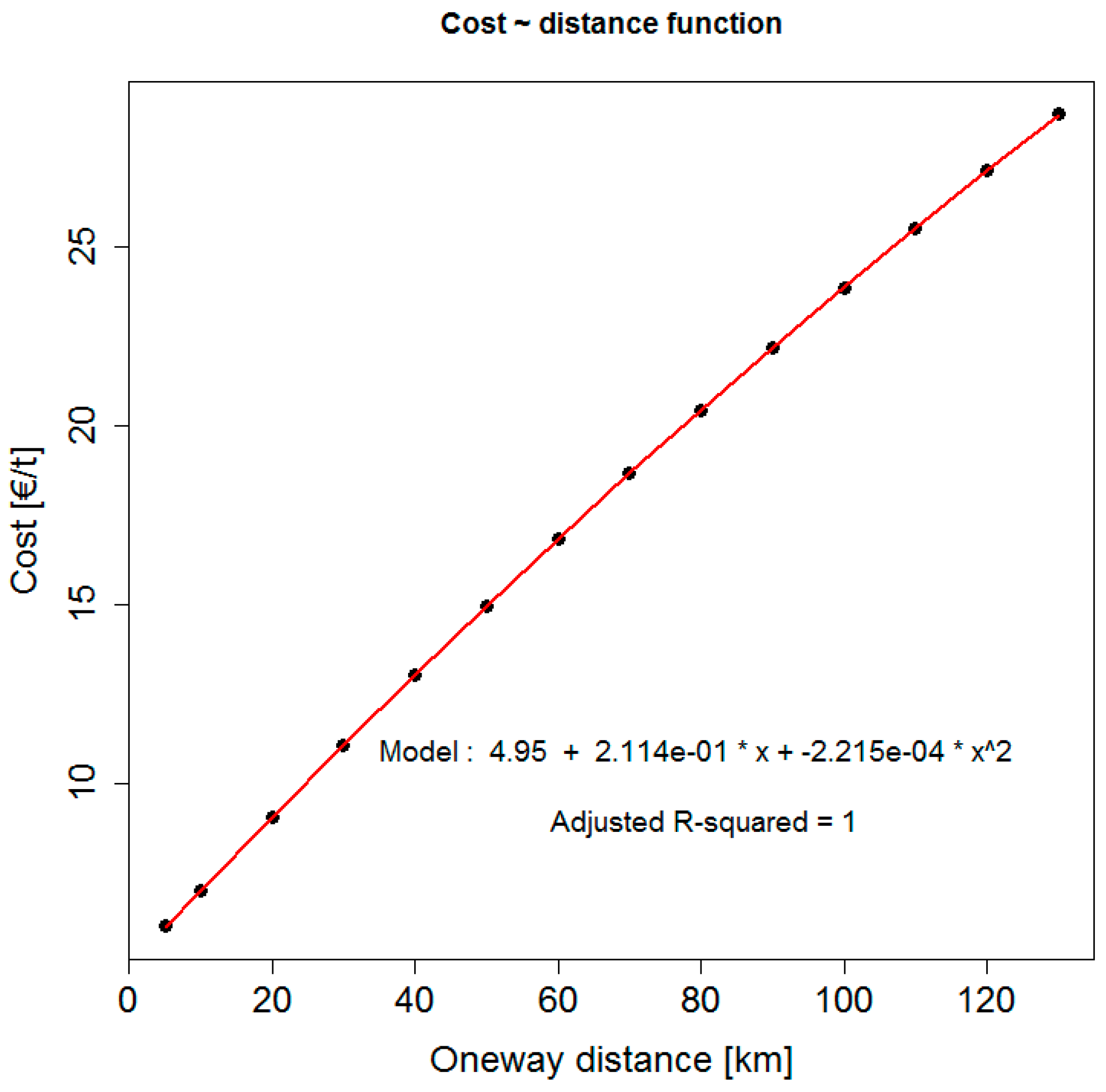
To convert timber volume (solid cubic meter) to Mg of dry biomass, we used a conversion factor of 1.866 m3 t−1 at 0% moisture derived from wood densities [29] for mixed softwood and hardwood weighted by the main tree species (abundance > 0.5%) from the third NFI data. Using distance and cost values, we built a simple linear model with a quadratic function (Figure 3). The model featured an r2 of ca. 1 and a RMSE of €0.01, thus allowing for precise fitting of all distance values in the given interval (5–130 km). We used this model to calculate costs according to actual mean transport distances within our service area (Table 4).
The mean transport range was calculated according to a circle as 2/3 the radius of maximum transport distance.

2.6. Timber Assortments and Pricing

Resource assortments and prices were the third crucial factor after the biomass potential and logistics for assessing the economic feasibility of an emerging bioeconomy. We based our estimation on available data supplied by the forest research institute of Baden-Württemberg [30]. These data covered state-owned forest (24% of the forest area) [22] from 2011–2016. The prices at which the timber was sold by the state forest administration were weighted by their relative shares to the assortments and attached to our quantities. To assess the economic feasibility of the positioning of conversion plants, transport and resource prices were estimated as follows: potentially relevant forest assortments as roundwood, fuelwood and pulpwood; and woody biomass from TOF as analogous to fuelwood. As such, 70% of the average annual harvest were roundwood (predominantly softwood), 14% pulpwood and 16% fuelwood (predominantly hardwood; Table 5).

3. Results

The results were built up in three steps. To get an initial overview, we started with the best positions in terms of biomass supply using catchment areas with five radii, biomass type and quality in three categories (Table 6). These values serve as a quick reference for a regional facility’s possible potential.
If wood type was not important, up to 3 million Mg of biomass could be acquired with a maximum transport distance of 50 km (Table 6). When specific wood type was considered, the overall potential dropped to 2 million Mg for softwood and 1.1 million Mg for hardwood. The potential also changed if we considered using only the cheaper wood assortments of fuel and pulpwood. While most coniferous timber was sold as high-value roundwood (~90%), a large share of hardwood was instead sold as fuel and pulpwood (~50% and ~25%, respectively). The potential of softwood consequently dropped from 2 to 0.22 million Mg, while the potential of hardwood only decreased from 1.1 to 0.85 million Mg. This revealed huge discrepancies between the theoretical and economic potential of biomass in the study area (−23% to −89%).

3.1. Scenarios

Since conversion and fraction technologies for lignocellulosic biomass are under development and a market is beginning to slowly emerge, we decided to build several scenarios to estimate the potential for a regional bioeconomy in Baden-Württemberg. The scenarios were simple and varied by usable resource type, timber assortment and facility size in terms of annual throughput. To estimate the effects of these variables on the positioning of regional lignocellulosic biomass conversion and fractioning facilities, we defined the following scenarios:
  • Very small facility (VSF) processing 20,000 Mg year−1 of woody biomass.
  • Small-size facility (SF) processing 80,000 Mg year−1 of woody biomass.
  • Medium-size facility (MF) processing 250,000 Mg year−1 of woody biomass.
There was a huge price difference between the high-quality roundwood and fuelwood and pulpwood (Table 5). Due to those differences in prices, we assumed it is not reasonable to process high-quality roundwood for bioeconomy products, and thus focused on the cheaper assortments of pulpwood and fuelwood in this analysis. First, we checked the feasibility of the suggested plant size in terms of resource availability. Yet to show the possible impact on the wood market, we calculated those results for three different resource use efficiencies (100%, 50%, 5%). A usage of 100% meant a complete, local displacement of fuelwood or pulpwood use by bioeconomy. The 50% scenario simulated coexistent wood usage as pulpwood, fuelwood and bioeconomy-wood. The last scenario was a no-impact/business-as-usual scenario using just a small share (5%) of the wood for bioeconomy.
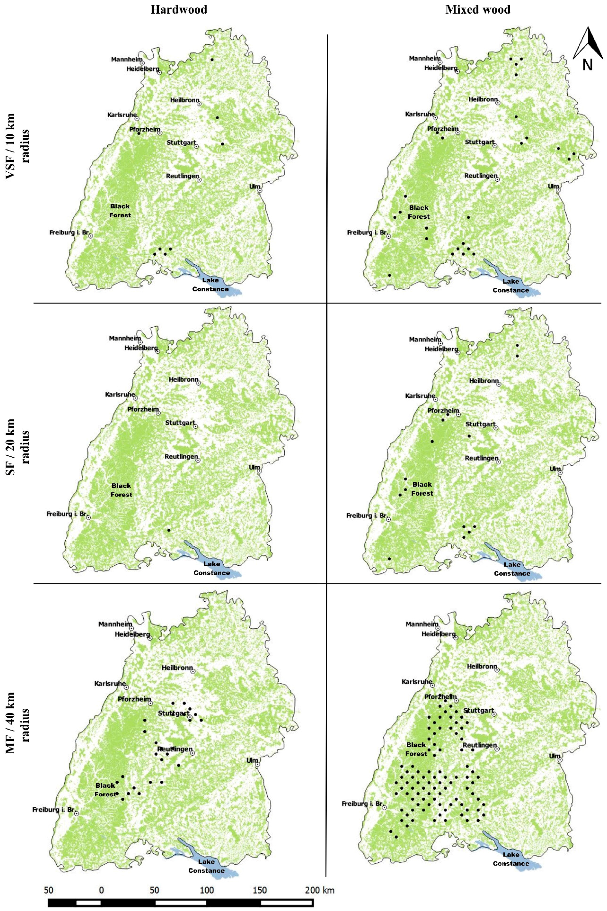
Without complete conversion (100%) or at least strong influence (50%) on the fuelwood and pulpwood market, only VSF were possible using hardwood or mixed wood with a minimum service area radius of 40 km (Table 7). As such, regional bioeconomy with transport distances of up to 50 km would compete with existing industries. Secondly, the regional (i.e., short distances) potential of low-price softwood was small, while, in comparison, the potential of cheap hardwood was high. Consequently, a bioeconomy seeking to minimise environmental impacts by primarily using regionally available biomass in Baden-Württemberg would need to focus on either hardwood or mixed wood. As those might be the most relevant scenarios, we calculated the optimal positions (see Figure 4) for hard- and mixed-wood processing facilities of all three sizes (VSF, SF, MF) using 50% of the available resources and minimal transport costs in terms of service area radii (Table 7).

3.2. Suitable Positions

In the final step, we filtered out all positions that did not provide the needed amount of resources for specific facility sizes using 50% of the available hardwood or mixed wood. Figure 4 shows the results of our positioning approach for six scenarios varying in wood type (hardwood or mixed wood), facility size (VSF, SF, MF) and service area radii (10, 20, 40 km) without competition between multiple facilities. For positioning competing facilities with overlapping service areas, a stepwise approach would be used to position one facility after the other. Thereby, the already used biomass would be excluded and is not available anymore for the next facilities.
For VSF using hardwood, only a few, wide-spread possible positions could be found across the federal state. The positions changed when conifers were included in our mixed-wood scenario. Specifically, the total number of possible positions rose and concentrated within forested areas such as the Black Forest.
The Southeast of the state between Ulm and Lake Constance showed limited potential for all different settings. For a SF with a 20 km supply radius as an example, only one position northwest of Lake Constance fitted the criteria. In contrast, many more positions became possible if the facility were able to process both wood types.
For a MF with a 40 km radius, the positions clumped in the centre of the federal state around Stuttgart, Reutlingen and southwest of the latter along the mid-east border of the Black Forest. There were a few positions spread throughout the Black Forest in the mid-north and again northwest of Lake Constance. For the mixed-wood scenario, numerous options were found in the Southeast (Black Forest, Germany) of the federal state.

3.3. Final Costs

Combining the results for transport and wood assortment, we calculated resource prices for the different scenarios. We first calculated mean prices for hardwood (90.04 € t−1) and softwood (82.65 € t−1) while excluding roundwood (Table 5). Since in the mixed scenarios the share of softwood varied (5–24%), the exact price was calculated individually for each position. For demonstration purposes though, we calculated the mean price of 89.08 € t−1 for mixed wood consisting of 13% softwood. When transportation costs were integrated for each scenario, we got a mean hardwood price of 96.36 € t−1 for VSF, €97.77 for SF and €100.47 for MF. Using mixed wood, we got prices of 95.43 € t−1 for VSF, €96.81 for SF and €99.51 for MF. The transportation cost had an impact on the final price between ca. 6.7% (5 km) and 31.9% (130 km) that increased roughly €1.8 every 10 km (Table 4). In our optimised scenarios, the share of the transportation in the overall biomass price was between 7.1 and 10.5%.

4. Conclusions

The potential biomass volumes, prices and facility positions resulting from our approach demonstrate the practical applicability of remote sensing-derived potential (in terms of biomass availability) maps to analyse the feasibility of a regional bioeconomy using lignocellulose. The explicit objective was to estimate the potential of a future bio-based economy to replace fossil-based chemicals, but in principle this method could be used for a wide variety of facilities from sawmills to pulp and paper mills to power and heating plants that use woody biomass. Similarly, it could be implemented anywhere on the globe.
While the produced results are based on a number of limited assumptions, this methodology for spatially explicit analysis outside those assumptions is possible. For instance, only data on lignocellulosic biomass from forests and TOF were included. Yet the study area could be easily expanded both spatially and to include other resource sources such as short rotation coppice. Spatial limits to such methods have decreased to the extent that global approaches (e.g., [31]) for mapping biomass have already been implemented; global timber harvest maps are only a matter of time.
The application of the methodology was straightforward in its combination of geo-referenced resource potential maps, infrastructure data and both transport and resource costs. The results demonstrated that, given the premises on transport distance and facilities’ throughput, the economic feasibility and possible location of a conversion plant can be easily checked.
The study clearly demonstrated, however, that large discrepancies between theoretic and economic potential exist. The results showed that up to 3 million Mg of lignocellulosic biomass were theoretically available at a maximum transport distance of 50 km. However, this potential changed dramatically when restrictions were implemented about the type of wood, timber assortment and share of the resource used. Should conversion processes be tolerant to mixed wood as input material though, more suitable positions would become available.
Alternatively, if the demand from a facility is more precisely defined, a more refined investigation could be performed. For instance, a single tree species like beech could be selected or the facility could be located close to sawmills, thus making use of existing infrastructure and possibly any by-products. About 40% of the roundwood processed in sawmills is considered waste as, e.g., wood chips and saw dust [32].
Other assumptions such as costs and demand are likely to change. We showed that facilities with a throughput of 20, 80 or 250 Gg year−1 fuelled by regionally produced biomass are economically possible at relative low transport costs (ca. 10% of the resource price). Yet, these were mean costs specifically calculated for Baden-Württemberg, and may change over time especially due to fluctuations in the price of fuel. Also, the suggested positions of facilities are located in regions with high biomass potential that meet our defined criteria. These criteria can and will need to be adapted according to implemented conversion technology and associated requirements for raw woody biomass.
Additional factors besides biomass cost and availability remain to be implemented such as specific infrastructure (e.g., a harbour or railway station), local tax situation, and political or social influence. These results indicate that an emerging bioeconomy using regionally produced biomass will directly compete with regional wood-fired combustion plants since resource price is currently low and transport costs strongly increase with distance. Thus, local wood prices can be expected to rise if bioeconomy demands large quantities of fuelwood. Whether it is possible to establish a bioeconomy depends on its competitiveness to fossil raw materials-based economy and a supportive governance [4].

Acknowledgments

This work was supported by a grant from the Ministry of Science, Research and the Arts of Baden-Württemberg (funding code: 7533-10-5-79) to all authors. The study was developed in cooperation with the Forest Research Institute Baden-Württemberg (FVA, www.fva-bw.de). We would like to thank Gerad Kändler and Christoph Hartebrodt of the FVA in Freiburg for providing data and helpful discussions. Felix Storch from the department of Silvicultures of the University of Freiburg shared once more his deep understanding of the National Forest Inventory data with us. Thomas Fillbrandt from the Chair of Forest Operations of the University of Freiburg also shared his experience and knowledge on forest engineering. We would like to thank OpenStreetMap© for providing open-source, high-quality data. Tobias Mathow and Wilfried Ressel of the forest administration (ForstBW, Freiburg, Germany) kindly provided the geodata about forested areas in Baden-Württemberg. Thanks to Kenton Stutz from the Chair of Soil Ecology at the University of Freiburg for his valuable feedback and proofreading.

Author Contributions

J.M., M.L., T.S., D.J. and B.K. conceived and designed the approach, J.M. performed the analysis; J.M., M.L. and T.S. analyzed the data; J.M., M.L. and T.S. contributed materials; J.M. prepared the paper, M.L., T.S., D.J. and B.K. further improved it.

Conflicts of Interest

The authors declare no conflict of interest.

References

  1. Federal Ministry of Education and Research (BMBF). Bioeconomy in Germany: Opportunities for a Bio-Based and Sustainable Future; Federal Ministry of Education and Research (BMBF): Berlin, Germany, 2015. [Google Scholar]
  2. European Association for Bioindustries (EuropaBio). Building a Bio-Based Economy for Europe in 2020; European Association for Bioindustries (EuropaBio): Brussels, Belgium, 2011. [Google Scholar]
  3. European Commission (EC). Innovating for Sustainable Growth: A Bioeconomy for Europe; European Commission (EC): Brussels, Belgium, 2012. [Google Scholar]
  4. Organisation for Economic Cooperation and Development (OECD). The Bioeconomy to 2030: Designing a Policy Agenda, Main Findings; Organisation for Economic Cooperation and Development (OECD): Paris, France, 2009. [Google Scholar]
  5. Federal Ministry of Education and Research (BMBF). Nationale Forschungsstrategie BioÖkonomie 2030—Unser Weg zu Einer Bio-Basierten Wirtschaft; Federal Ministry of Education and Research (BMBF): Berlin, Germany, 2010. [Google Scholar]
  6. German Presidency. En Route to the Knowledge-Based Bio-Economy; German Presidency: Cologne, Germany, 2007. [Google Scholar]
  7. Langeveld, J.W.; Sanders, J.P.M. The Biobased Economy: Biofuels, Materials and Chemicals in the Post-Oil Era; Langeveld, H., Sanders, J., Meeusen, M., Eds.; Earthscan: London, UK, 2012. [Google Scholar]
  8. Rudel, T.K.; Coomes, O.T.; Moran, E.; Achard, F.; Angelsen, A.; Xu, J.; Lambin, E. Forest transitions: Towards a global understanding of land use change. Glob. Environ. Chang. 2005, 15, 23–31. [Google Scholar] [CrossRef]
  9. Treuhaft, R.N.; Asner, G.P.; Law, B.E. Structure-based forest biomass from fusion of radar and hyperspectral observations. Geophys. Res. Lett. 2003, 30. [Google Scholar] [CrossRef]
  10. Alam, M.B.; Shahi, C.; Pulkki, R. Wood biomass supply model for bioenergy production in Northwestern Ontario. In Proceedings of the 1st International Conference on the Developments in Renewable Energy Technology (ICDRET), Dhaka, Bangladesh, 17–19 December 2009; pp. 1–3. [Google Scholar]
  11. Chinese, D.; Meneghetti, A. Optimisation models for decision support in the development of biomass-based industrial district-heating networks in Italy. Appl. Energy 2005, 82, 228–254. [Google Scholar] [CrossRef]
  12. Han, S.K.; Murphy, G.E. Solving a woody biomass truck scheduling problem for a transport company in Western Oregon, USA. Biomass Bioenergy 2012, 44, 47–55. [Google Scholar] [CrossRef]
  13. Kanzian, C.; Holzleitner, F.; Stampfer, K.; Ashton, S. Regional energy wood logistics-optimizing local fuel supply. Silva Fenn. 2009, 43, 113–128. [Google Scholar] [CrossRef]
  14. Freppaz, D.; Minciardi, R.; Robba, M.; Rovatti, M.; Sacile, R.; Taramasso, A. Optimizing forest biomass exploitation for energy supply at a regional level. Biomass Bioenergy 2004, 26, 15–25. [Google Scholar] [CrossRef]
  15. Frombo, F.; Minciardi, R.; Robba, M.; Rosso, F.; Sacile, R. Planning woody biomass logistics for energy production: A strategic decision model. Biomass Bioenergy 2009, 33, 372–383. [Google Scholar] [CrossRef]
  16. Keirstead, J.; Samsatli, N.; Pantaleo, A.M.; Shah, N. Evaluating biomass energy strategies for a UK eco-town with an MILP optimization model. Biomass Bioenergy 2012, 39, 306–316. [Google Scholar] [CrossRef] [Green Version]
  17. Rauch, P.; Gronalt, M. The effects of rising energy costs and transportation mode mix on forest fuel procurement costs. Biomass Bioenergy 2011, 35, 690–699. [Google Scholar] [CrossRef]
  18. Ragauskas, A.J.; Williams, C.K.; Davison, B.H.; Britovsek, G.; Cairney, J.; Eckert, C.A.; Frederick, W.J.; Hallett, J.P.; Leak, D.J.; Liotta, C.L.; et al. The path forward for biofuels and biomaterials. Science 2006, 311, 484–489. [Google Scholar] [CrossRef] [PubMed]
  19. Richardson, B. From a fossil-fuel to a biobased economy: The politics of industrial biotechnology. Environ. Plan. C Gov. Policy 2012, 30, 282–296. [Google Scholar] [CrossRef]
  20. Maack, J.; Lingenfelder, M.; Weinacker, H.; Koch, B. Modelling the standing timber volume of Baden-Württemberg—A large-scale approach using a fusion of Landsat, airborne LiDAR and National Forest Inventory data. Int. J. Appl. Earth Obs. Geoinform. 2016, 49, 107–116. [Google Scholar] [CrossRef]
  21. Maack, J.; Lingenfelder, M.; Eilers, C.; Smaltschinski, T.; Weinacker, H.; Jaeger, D.; Koch, B. Estimating the spatial distribution, extent and potential lignocellulosic biomass supply of Trees Outside Forests in Baden-Wuerttemberg using airborne LiDAR and OpenStreetMap data. Int. J. Appl. Earth Obs. Geoinform. 2017, 58, 118–125. [Google Scholar] [CrossRef]
  22. Kändler, G.; Cullmann, D. Der Wald in Baden-Württemberg. In Ausgewählte Ergebnisse der Dritten Bundeswaldinventur; Forstliche Versuchs- und Forschungsanstalt Baden-Württemberg: Freiburg, Germany, 2014. [Google Scholar]
  23. Wood, S.N. Generalized Additive Models: An Introduction with R; Chapman and Hall/CRC Press: Boca Raton, FL, USA, 2006. [Google Scholar]
  24. Chambers, J.M.; Hastie, T.J. Statistical models. In Scientific Modeling and Simulation SMNS; Springer: Dordrecht, The Netherlands, 1992. [Google Scholar]
  25. European Environment Agency (EEA). Corine Land Cover (CLC) 2012. Available online: http://land.copernicus.eu/pan-european/corine-land-cover/clc-2012/view (accessed on 15 November 2017).
  26. Reich, T.; Bernhard, J.; Geimer, M. Fahrzeugsystemtechnik. Karlsruher Institut für Technologie. In Optimierung des Holztransports in Baden-Württemberg; Arbeitsgemeinschaft Rohholzverbraucher: Berlin, Germany, 2015. [Google Scholar]
  27. Deutsche Bank. Personal Communication; Deutsche Bank: Frankfurt, Germany, 2017. [Google Scholar]
  28. Klenk, A. Analyse Konkreter Rundholztransporte. Bachelor’s Thesis, Hochschule für Forstwirtschaft Rottenburg, Neckar, Germany, 2015. [Google Scholar]
  29. Wagenfuehr, R. Holzatlas; Fachbuchverlag Leipzig, Hanser: Munich, Germany, 2000; ISBN 3-446-21390-2. [Google Scholar]
  30. Forest Research Institute Baden-Württemberg (FVA). Personal Communication; Forest Research Institute Baden-Württemberg (FVA): Breisgau, Germany, 2017. [Google Scholar]
  31. Le Toan, T.; Quegan, S.; Davidson, M.W.J.; Balzter, H.; Paillou, P.; Papathanassiou, K.; Plummer, S.; Rocca, F.; Saatchi, S.; Shugart, H.; et al. The BIOMASS mission: Mapping global forest biomass to better understand the terrestrial carbon cycle. Remote Sens. Environ. 2011, 115, 2850–2860. [Google Scholar] [CrossRef]
  32. Sörgel, C.; Mantau, U.; Weimar, H. Standorte der Holzwirtschaft—Aufkommen von Sägenebenprodukten und Hobelspänen; Arbeitsbereich Ökonomie der Holz- und Forstwirtschaft, Universität Hamburg Zentrum Holzwirtschaft: Hamburg, Germany, 2006. [Google Scholar]
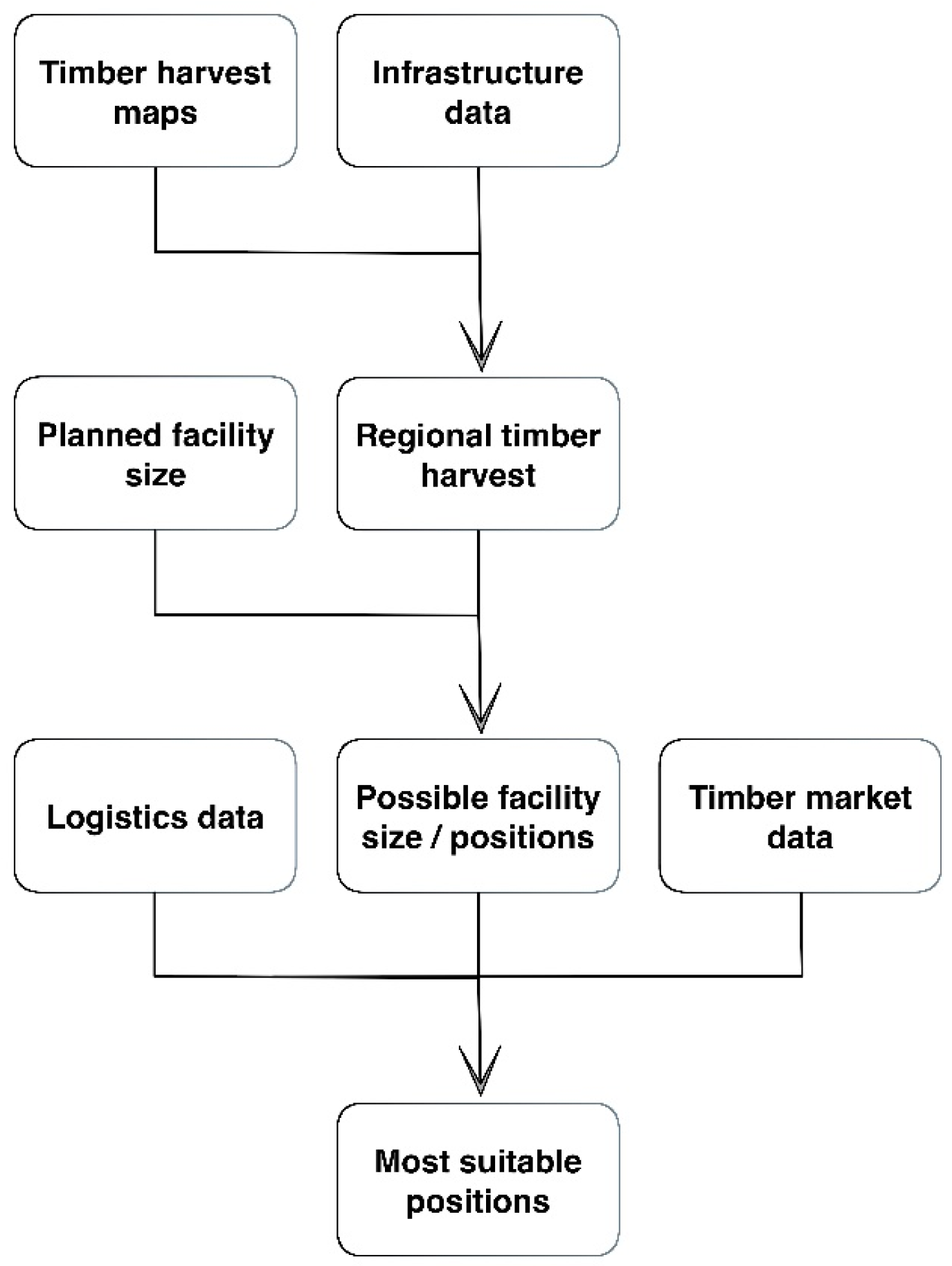
Figure 1. Simplified workflow of the approach showing necessary data and intermediate results for finding the most suitable facility positions.
Forests 08 00449 g001
Figure 2. Study area Baden-Württemberg (black) located in southwest Germany (grey).
Forests 08 00449 g002
Figure 3. Linear model with 2nd degree polynomic function (red line) modelling the relationship between transport distance and cost per dry Mg of woody biomass. Data points are the black dots.
Forests 08 00449 g003
Figure 4. The federal state of Baden-Württemberg: vegetation in green, large lakes in blue, cities > 100,000 inhabitants as white circles labelled with their name. The suitable positions for the six scenarios are shown as black dots.
Forests 08 00449 g004
Table 1. General acquisition, operation and personnel costs. Data basis from Reich et al. [26], assuming a price increase of 2% for vehicles since 2015.
ItemValue
Tractor unit, crane, trailer172,400
Annual mileage96,718km
Annual operating days248days
Fuel price per liter1.25
Fuel consumption per 100 km47l
Tire cost per km0.058
Lubricant costs per km0.022
Road toll per km0.130
Maintenance and repair per km0.101
Personnel costs (including social contributions) per month for the driver3600
Table 2. Calculated annual expenses according to Reich et al. [26] except for fuel and labor costs.
Cost TypeCost ItemValue (€ year−1)
Variable costsFuel56,870
Tires5562
Lubricant2100
Maintenance and repair9751
Sum variable costs74,283
Fixed costsAnnual credit rate (4%)31,607
Vehicle tax1500
Vehicle insurance3500
Road toll4523
Other test costs400
Mobile phone and internet600
Sum fix costs42,130
Personnel costsSalary plus social security contributions43,200
Impute costsAdministrative costs3000
Company risk12,000
Sum impute costs15,000
All costsSum of all costs174,613
Table 3. Transportation speed and cost for distances between 5 and 130 km.
Distance (km)
One-WayForest Road Speed Limit 60 km h−1 Speed Limit 80 km h−1 Mean Speed (km h−1)Trips Per Day (n)Costs Per m3 (€)Costs Per Mg (Dry) (€)
52.72.30.035.08.13.236.03
102.77.30.042.66.93.767.02
202.716.80.647.25.44.869.07
302.725.71.749.14.45.9411.09
402.734.03.350.53.77.0013.06
502.741.85.551.63.28.0314.98
602.749.18.352.52.99.0316.85
702.755.811.653.42.610.0018.67
802.761.915.454.22.410.9620.44
902.767.519.855.02.211.8822.18
1002.772.624.855.82.012.7923.87
1102.777.130.356.61.913.6725.52
1202.781.036.357.31.814.5427.13
1302.784.442.958.11.715.3828.70
Table 4. Fitted tariff for varying service area sizes.
Radius Service Area (km)Mean Distance One Way (km)Fitted Costs Per Mg (Dry) (€)
106.676.35
2013.337.73
3020.009.09
4026.6710.43
5033.3311.75
Table 5. Selling price and share of wood from forests (average 2011–2016) by type and assortment.
TypeClassRelative Share of Annual Harvest (%)Relative Share of Annual Harvest by Wood Class (%)Sales Price (€ m−3)Sales Price (€ Mg−1 (Dry))
HardwoodFuelwood15.250.749.291.8
Pulpwood7.82646.486.6
Roundwood7.023.382.6154.1
SoftwoodFuelwood0.71.026.248.9
Pulpwood6.39.046.386.4
Roundwood62.990.080.7150.6
Table 6. Potential biomass from the positions with the highest annual harvest.
Radius Service Area (km)Softwood (Mg year−1)Hardwood (Mg year−1)Mixed Wood (Mg year−1)Transport Cost (€ Mg−1)
AllFuelPulpAllFuelPulpAllFuelPulp
10114,852279310,31655,73029,72913,838149,48731,75420,7016.35
20375,399801833,620214,059114,08853,046522,973119,67573,2187.73
30833,68616,15774,534415,518225,925100,6001,182,900239,236162,6809.09
401,435,26327,939128,152681,646371,476164,5802,087,763395,820288,95610.43
502,013,98241,078179,4281,092,278584,652269,3523,074,860623,060446,09511.75
Table 7. Minimal service area radius in relation to facility size (VSF = 20 Gg year−1, SF = 80 Gg year−1, MF = 250 Gg year−1), resource (fuelwood and pulpwood only) and usage (100%, 50%, 5%).
Min. Service Area Radius (km)
100% Resources Usage50% Resources Usage5% Resources Usage
Soft-WoodHard-WoodMixed WoodSoft-WoodHard-WoodMixed WoodSoft-WoodHard-WoodMixed Wood
VSF201010201010-4040
SF302020502020---
MF-3030-4040---