A Simulation of Image-Assisted Forest Monitoring for National Inventories

Abstract

The efficiency of national forest monitoring efforts can be increased by the judicious incorporation of ancillary data. For instance, a fixed number of ground plots might be used to inform a larger set of annual estimates by observing a smaller proportion of the plots each year while augmenting each annual estimate with ancillary data in order to reduce overall costs while maintaining a desired level of accuracy. Differencing successive geo-rectified remotely sensed images can conceivably provide forest change estimates at a scale and level of accuracy conducive to the improvement of temporally relevant forest attribute estimates. Naturally, the degree of improvement in the desired estimates is highly dependent on the relationships between the spatial-temporal scales of ground plot and remotely sensed observations and the desired spatial-temporal scale of estimation. In this paper, fixed scales of observation for each data source are used to explore the value of three different levels of information available from the remotely sensed image-change estimates. Four populations are simulated and sampled under four sampling error structures. The results show that the image change estimates (ICE) can be used to significantly reduce bias for annual estimates of harvest and mortality and that improved estimation of harvest and mortality can sometimes, but not always, contribute to better estimates of standing volume.

1. Introduction

The efficiency of national forest inventory (NFI) efforts can be increased by the judicious incorporation of ancillary data. For instance, ancillary data can be used to lengthen the time it takes to collect the ground plot data in order to reduce overall costs while maintaining a desired level of accuracy. Roesch et al. [1] showed that the inclusion of auxiliary data that is more temporally dense than the ground plot data has the potential to provide improvement in estimation if time is specifically accounted for in the estimation process. This conclusion is, of course, highly dependent upon the inter-relationships of temporal scales of both observation and estimation. Here, I further investigate the relationships between the scales of ground plot and remotely sensed observation with the scale of estimation in the presence of realistic levels of sampling and measurement error. These inter-relationships of scale and error have many implications when one is attempting to optimize sample designs.

Eastaugh and Hasenauer [2] gave the results of an uncommonly thorough investigation into the bias that can be introduced into theoretically unbiased estimators under plausible assumptions concerning common sampling and measurement errors in remeasured forest inventories. In the current investigation, estimator performance was tested in a simulation designed to consider a wide range of potential sampling and measurement errors. Within the simulation, I use four sampling error structures for the measured plot data and three levels of availability of the remotely sensed image change estimates (ICE).

Ultimately, my objective is to obtain improvements in annual estimates of the components of change and standing cubic-meter volume, given both the multi-year data arising from temporally overlapping panels of plot observations and more frequent observations by remote sensing. Without loss of generality, the sample design for the plot observations used here is one option of an interpenetrating, panelized annual inventory system, such as the one defined by the USDA Forest Service’s Forest Inventory and Analysis (FIA) Program, and presented in Bechtold and Patterson [3]. The general aspects of the interpenetrating design originated in the United States in the Forest Health Monitoring (FHM) Program in the late 1980s, while some of the FIA units began using the design in 1998 until, soon after, it became the official national design. Since then many other countries have incorporated interpenetrating designs, while still others are considering the use of such designs (see e.g., Massey et al. [4]; Vidal et al. [5]). Here, I set the cycle length for the plot observations to ten years, and the interval of remotely sensed ICE observations to two years, as explained below.

Minimally, ICE observations should provide an improved knowledge of the spatial and temporal location of harvests, obtainable through the ground plot observations. To a lesser extent, we might expect the same to be true for mortality events. Given the scale of national forest inventories, estimates of harvest and mortality that are unaided by auxiliary data typically have higher than desired variances. In order to join these disparate data sources, I rely on the discrete components of change definitions of Roesch [6] and investigate how well improvements in the estimation of the harvest and mortality components can lead to improvements in the estimation of annual volume. Forest monitoring can be described in many contexts, but it is important to note that the major difference between the ideas of forest monitoring and the more traditional forest inventory is that, in the former, the major emphasis is to observe the forests as they are changing, while in the latter the major emphasis was to describe the forests at particular points in time, possibly separated by five, ten, or more years, and the change that had occurred in the interim. The difference may seem like nuance, but it leads to entirely different forest estimation paradigms. For a comprehensive discussion of potential monitoring paradigms, the reader is referred to Corona [7].

The definitions of the components of change used here more closely follow a monitoring paradigm than an inventory paradigm as they are applied annually and are derived from the more general definitions of Eriksson [8], which apply to any period of time. In the Eriksson [8] definitions, entry is the cubic meter volume (or other measure of value) of trees as they attain the entry criterion; Live growth is the annual growth in volume of trees in the population; mortality is the volume of trees as they die; and harvest is the volume of trees as they are harvested. These components are unique and mutually exclusive and, when they are applied annually, they sum to the total annual change:

$$Y_{\mathit{t}+1}=Y_{\mathit{t}}+L_{\mathit{t}}+E_{\mathit{t}}-M_{\mathit{t}}-H_{\mathit{t}}$$

(1)

where:

• Y_t = the volume at the beginning of year t,
• L_t = live growth during year t,
• E_t = entry during year t,
• M_t = mortality during year t, and
• H_t = harvest during year t.

If the estimates of these components combine annually in the same manner, they are also considered to be compatible. The compatible recursive estimation systems explored in Roesch et al. [1] are used here with attention being paid to estimates of the harvest, mortality, entry and live growth components with respect to how they combine to form estimates of annual volume.

2. Materials and Methods

2.1. Simulated Populations

I constructed four simulated populations, the first of which had also been used and described in Roesch et al. [1]. These populations are intended to examine estimator performance in the presence of a wider but still plausible set of suboptimal and latent population characteristics, in the form of nonlinear trends and fine-scale anomalies. A similar approach using different seed data and error assumptions was exploited in Roesch [9]. The seed data for this study came from FIA plot data measured at least twice in the state of Georgia (USA) between 1995 and 2012, consisting of 7330 ground plots (set 1), most of which had two observed growth intervals for each component with remeasurement intervals that varied quite widely around the five-year target for these plots. First a null population (population 0) was constructed to represent a reasonable facsimile to the population of forested conditions from which set 1 could have been drawn. Population 0 consisted of 500 variance-interjected copies of set 1, resulting in a population of 3,665,000 hectares, of which 2,360,411 were forested at some time during the period of interest. The variance was interjected at two levels. In level 1, in order to maintain trend while adding variance to the seed, all values for each component on each hectare were multiplied by a unique random variate, drawn from an N(1, 0.025) distribution. The second level of variance was introduced temporally by multiplying the result of step 1 for each annual value for each component on each hectare by a unique random variate drawn from an N(1, 0.0025) distribution. The four test populations, 1 through 4, were then constructed from population 0. For each population, trend was introduced through the application of the formula:

$${\mathit{\epsilon }}_{\mathit{t}}=\mathbf{\left[}\mathbf{\alpha }\mathbf{+}\mathbf{\left(}\mathbf{\beta }\mathbf{ln}\mathbf{(}\mathit{t}\mathbf{-}\mathbf{1997}\mathbf{\right)}\mathbf{\right]}\mathbf{,}\mathit{t}\mathbf{=}\mathbf{1998}\mathbf{to}\mathbf{2011}$$

(2)

For population 1, a mild (latent) nonlinear trend was introduced into each of the components of population 0 by multiplying each value in each year t by ε_t in (2) after setting $\mathbf{\alpha }=\mathbf{0.95}$ and $\mathbf{\beta }=\mathbf{0.05}$. Population 2 was constructed similarly to Population 1 except that increased harvesting pressure was introduced by setting $\mathbf{\alpha }=\mathbf{0.90}$ and $\mathbf{\beta }=\mathbf{0.10}$ for the harvest component. Population 3 was constructed as in Population 1, except with an introduced catastrophic event of four times the amount of mortality of Population 1 in 2004. Population 4 was initially constructed in the same manner as Population 0 and then postulated climate change effects were simulated by increasing mortality and decreasing growth and recruitment, with harvest levels remaining the same as in Population 1. Although the potential rates of change are unknown and arbitrarily set for the purposes of this study, the justification for this effect comes from a general principle in ecology that assumes all species have a range of tolerance for any environmental factor (see e.g., Smith [10]). Some of the members of any species exist near the edge of one or more of those ranges of tolerances. If climate changes in any way, some of the members of a species that cannot move will be in one or more out-of-tolerance zones, possibly resulting in decreasing growth and fecundity and increasing mortality. For live growth, $\mathsf{\alpha }$ was set equal to 0.90 and $\mathsf{\beta }$ was set equal to −0.10. For entry, $\mathsf{\alpha }$ was set equal to 0.95 and $\mathsf{\beta }$ was set equal to −0.05, and for mortality, $\mathsf{\alpha }$ was set equal to 0.80 and $\mathsf{\beta }$ was set equal to 0.20. For clarity, these parameters values for each population are given in

Table 1. The parameters (α and β) of Equation (2) used to simulate each population of entry (E), live growth (L), mortality (M) and harvest (H). (The increase in mortality, by a factor of four, for Population 3 in 2004 is not represented in the table.)

Component	Population
	1		2		3		4
	α	β	α	β	α	β	α	β
E	0.95	0.05	0.95	0.05	0.95	0.05	0.95	−0.05
L	0.95	0.05	0.95	0.05	0.95	0.05	0.90	−0.10
M	0.95	0.05	0.95	0.05	0.95	0.05	0.80	0.20
H	0.95	0.05	0.90	0.10	0.95	0.05	0.95	0.05

.

Table A1. Distribution statistics for population 1.

		Year
Component	Statistic	1998	1999	2000	2001	2002	2003	2004	2005	2006	2007	2008	2009	2010	2011
Volume	Minimum	0.00	0.00	0.00	0.00	0.00	0.00	0.00	0.00	0.00	0.00	0.00	0.00	0.00	0.00
	1st Quartile	0.00	0.00	0.42	1.89	4.33	7.11	9.86	12.56	14.84	16.47	17.58	18.59	19.17	19.59
	Median	9.91	14.93	19.98	25.31	30.71	35.84	41.21	45.78	49.51	53.05	56.53	59.07	61.52	63.46
	Mean	50.53	54.21	57.79	61.45	65.60	69.50	73.21	76.16	78.78	81.30	83.62	85.70	87.46	89.00
	3rd Quartile	77.83	83.76	89.56	95.08	101.26	106.63	110.80	113.99	116.78	120.38	123.21	126.65	130.25	132.89
	Maximum	813.34	813.36	814.69	815.08	816.37	818.58	821.72	825.90	831.01	837.24	844.48	852.75	862.01	872.21
Live Growth	Minimum	0.00	0.00	0.00	0.00	0.00	0.00	0.00	0.00	0.00	0.00	0.00	0.00	0.00	0.00
	1st Quartile	0.00	0.00	0.00	0.00	0.29	0.66	0.73	0.66	0.50	0.22	0.00	0.00	0.00	0.00
	Median	1.19	1.49	2.02	2.49	3.04	3.36	3.43	3.40	3.36	3.20	2.35	0.73	0.00	0.00
	Mean	3.57	3.59	3.79	4.01	4.27	4.43	4.49	4.47	4.48	4.53	4.13	3.51	2.75	1.71
	3rd Quartile	5.30	5.39	5.70	6.03	6.35	6.50	6.65	6.68	6.72	6.94	6.56	5.65	3.94	0.00
	Maximum	52.52	50.58	66.35	58.15	48.79	39.41	33.73	35.04	39.47	43.90	44.57	41.38	39.08	46.09
Entry	Minimum	0.00	0.00	0.00	0.00	0.00	0.00	0.00	0.00	0.00	0.00	0.00	0.00	0.00	0.00
	1st Quartile	0.00	0.00	0.00	0.00	0.00	0.00	0.00	0.00	0.00	0.00	0.00	0.00	0.00	0.00
	Median	0.00	0.04	0.11	0.17	0.22	0.25	0.26	0.24	0.22	0.18	0.08	0.00	0.00	0.00
	Mean	0.45	0.47	0.52	0.57	0.62	0.64	0.65	0.64	0.63	0.64	0.57	0.47	0.35	0.22
	3rd Quartile	0.46	0.50	0.58	0.64	0.72	0.76	0.78	0.75	0.72	0.67	0.56	0.38	0.16	0.00
	Maximum	21.21	21.60	29.03	27.63	17.04	12.20	9.91	11.56	13.28	15.23	16.71	15.15	15.01	14.90
Mortality	Minimum	0.00	0.00	0.00	0.00	0.00	0.00	0.00	0.00	0.00	0.00	0.00	0.00	0.00	0.00
	1st Quartile	0.00	0.00	0.00	0.00	0.00	0.00	0.00	0.00	0.00	0.00	0.00	0.00	0.00	0.00
	Median	0.00	0.00	0.00	0.00	0.00	0.03	0.06	0.06	0.02	0.00	0.00	0.00	0.00	0.00
	Mean	0.74	0.74	0.76	0.78	0.82	0.86	0.88	0.91	0.94	0.97	0.90	0.77	0.60	0.38
	3rd Quartile	0.21	0.28	0.39	0.46	0.55	0.65	0.71	0.73	0.72	0.69	0.48	0.20	0.00	0.00
	Maximum	108.46	93.27	78.00	77.97	78.57	78.77	79.11	79.44	79.54	80.31	80.39	80.51	80.83	80.94
Harvest	Minimum	0.00	0.00	0.00	0.00	0.00	0.00	0.00	0.00	0.00	0.00	0.00	0.00	0.00	0.00
	1st Quartile	0.00	0.00	0.00	0.00	0.00	0.00	0.00	0.00	0.00	0.00	0.00	0.00	0.00	0.00
	Median	0.00	0.00	0.00	0.00	0.00	0.00	0.00	0.00	0.00	0.00	0.00	0.00	0.00	0.00
	Mean	0.63	0.75	0.84	0.99	1.21	1.45	1.78	1.99	2.16	2.20	1.90	1.55	1.05	0.55
	3rd Quartile	0.00	0.00	0.00	0.00	0.00	0.00	0.00	0.00	0.00	0.00	0.00	0.00	0.00	0.00
	Maximum	341.31	373.88	352.31	358.61	447.97	466.30	466.29	462.06	465.60	483.98	485.19	498.90	488.34	510.38

,

Table A2. Distribution statistics for population 2.

		Year
Component	Statistic	1998	1999	2000	2001	2002	2003	2004	2005	2006	2007	2008	2009	2010	2011
Volume	Minimum	0.00	0.00	0.00	0.00	0.00	0.00	0.00	0.00	0.00	0.00	0.00	0.00	0.00	0.00
	1st Quartile	0.00	0.00	0.40	1.84	4.23	6.96	9.60	12.18	14.36	15.85	16.85	17.75	18.27	18.47
	Median	9.92	14.91	19.91	25.21	30.56	35.64	40.95	45.44	49.13	52.52	55.81	58.18	60.61	62.44
	Mean	50.54	54.21	57.77	61.40	65.48	69.34	72.98	75.87	78.39	80.81	83.02	85.02	86.69	88.18
	3rd Quartile	77.85	83.75	89.54	95.06	101.16	106.48	110.52	113.66	116.30	119.70	122.36	125.71	129.16	131.71
	Maximum	817.12	817.14	818.39	818.81	820.10	822.27	825.34	829.30	834.12	840.11	847.13	855.06	864.06	873.90
Live Growth	Minimum	0.00	0.00	0.00	0.00	0.00	0.00	0.00	0.00	0.00	0.00	0.00	0.00	0.00	0.00
	1st Quartile	0.00	0.00	0.00	0.00	0.29	0.66	0.72	0.66	0.49	0.20	0.00	0.00	0.00	0.00
	Median	1.19	1.49	2.02	2.49	3.04	3.35	3.43	3.40	3.36	3.20	2.34	0.73	0.00	0.00
	Mean	3.57	3.59	3.79	4.01	4.27	4.43	4.49	4.46	4.47	4.52	4.13	3.51	2.75	1.71
	3rd Quartile	5.30	5.39	5.70	6.03	6.35	6.50	6.65	6.68	6.72	6.94	6.55	5.64	3.93	0.00
	Maximum	53.14	50.99	64.66	57.50	48.22	38.87	34.09	35.12	39.56	44.20	44.79	41.08	39.22	47.07
Entry	Minimum	0.00	0.00	0.00	0.00	0.00	0.00	0.00	0.00	0.00	0.00	0.00	0.00	0.00	0.00
	1st Quartile	0.00	0.00	0.00	0.00	0.00	0.00	0.00	0.00	0.00	0.00	0.00	0.00	0.00	0.00
	Median	0.00	0.04	0.11	0.17	0.22	0.25	0.26	0.24	0.21	0.18	0.07	0.00	0.00	0.00
	Mean	0.45	0.47	0.52	0.57	0.61	0.64	0.65	0.64	0.63	0.64	0.57	0.47	0.35	0.22
	3rd Quartile	0.46	0.49	0.58	0.64	0.72	0.76	0.77	0.75	0.72	0.67	0.55	0.38	0.16	0.00
	Maximum	21.51	22.06	29.05	27.55	16.99	12.11	9.90	11.63	13.32	15.21	16.64	15.13	14.87	14.81
Mortality	Minimum	0.00	0.00	0.00	0.00	0.00	0.00	0.00	0.00	0.00	0.00	0.00	0.00	0.00	0.00
	1st Quartile	0.00	0.00	0.00	0.00	0.00	0.00	0.00	0.00	0.00	0.00	0.00	0.00	0.00	0.00
	Median	0.00	0.00	0.00	0.00	0.00	0.03	0.06	0.06	0.02	0.00	0.00	0.00	0.00	0.00
	Mean	0.74	0.74	0.76	0.78	0.82	0.86	0.88	0.91	0.94	0.97	0.90	0.76	0.60	0.38
	3rd Quartile	0.21	0.28	0.39	0.46	0.55	0.65	0.71	0.73	0.72	0.69	0.48	0.20	0.00	0.00
	Maximum	109.16	93.88	78.48	77.31	77.80	78.08	78.46	78.55	78.85	79.36	79.29	80.21	79.93	80.14
Harvest	Minimum	0.00	0.00	0.00	0.00	0.00	0.00	0.00	0.00	0.00	0.00	0.00	0.00	0.00	0.00
	1st Quartile	0.00	0.00	0.00	0.00	0.00	0.00	0.00	0.00	0.00	0.00	0.00	0.00	0.00	0.00
	Median	0.00	0.00	0.00	0.00	0.00	0.00	0.00	0.00	0.00	0.00	0.00	0.00	0.00	0.00
	Mean	0.63	0.75	0.84	0.99	1.21	1.45	1.78	1.99	2.16	2.20	1.90	1.55	1.05	0.55
	3rd Quartile	0.00	0.00	0.00	0.00	0.00	0.00	0.00	0.00	0.00	0.00	0.00	0.00	0.00	0.00
	Maximum	341.31	373.88	352.31	358.61	447.97	466.30	466.29	462.06	465.60	483.98	485.19	498.90	488.34	510.38

,

Table A3. Distribution statistics for population 3.

		Year
Component	Statistic	1998	1999	2000	2001	2002	2003	2004	2005	2006	2007	2008	2009	2010	2011
Volume	Minimum	0.00	0.00	0.00	0.00	0.00	0.00	0.00	0.00	0.00	0.00	0.00	0.00	0.00	0.00
	1st Quartile	0.00	0.01	0.53	2.20	4.87	8.04	9.14	10.45	13.06	14.71	15.80	16.81	17.40	17.79
	Median	10.75	16.13	20.67	25.56	30.53	36.24	40.04	43.26	47.86	51.44	54.68	57.17	59.44	61.53
	Mean	51.18	54.72	58.13	61.61	65.57	69.84	72.10	73.23	76.58	79.13	81.51	83.61	85.38	86.95
	3rd Quartile	78.58	83.99	89.65	94.95	101.07	106.52	109.36	110.52	114.31	117.73	120.77	124.18	128.08	130.65
	Maximum	810.43	810.45	811.78	812.27	813.73	816.17	819.60	812.08	817.60	824.27	832.04	840.86	850.77	861.88
Live Growth	Minimum	0.00	0.00	0.00	0.00	0.00	0.00	0.00	0.00	0.00	0.00	0.00	0.00	0.00	0.00
	1st Quartile	0.00	0.00	0.00	0.00	0.36	0.69	0.63	0.36	0.42	0.12	0.00	0.00	0.00	0.00
	Median	1.24	1.54	2.08	2.55	3.09	3.34	3.38	3.24	3.31	3.14	2.29	0.65	0.00	0.00
	Mean	3.64	3.64	3.83	4.05	4.31	4.42	4.45	4.35	4.44	4.48	4.10	3.48	2.73	1.70
	3rd Quartile	5.40	5.48	5.78	6.10	6.39	6.48	6.61	6.59	6.68	6.90	6.52	5.59	3.89	0.00
	Maximum	53.47	51.13	65.89	57.70	48.59	39.46	33.90	34.73	39.03	43.61	45.57	41.61	39.45	46.75
Entry	Minimum	0.00	0.00	0.00	0.00	0.00	0.00	0.00	0.00	0.00	0.00	0.00	0.00	0.00	0.00
	1st Quartile	0.00	0.00	0.00	0.00	0.00	0.00	0.00	0.00	0.00	0.00	0.00	0.00	0.00	0.00
	Median	0.01	0.04	0.12	0.17	0.22	0.25	0.25	0.22	0.21	0.17	0.07	0.00	0.00	0.00
	Mean	0.46	0.48	0.53	0.58	0.62	0.64	0.64	0.62	0.63	0.63	0.56	0.47	0.35	0.22
	3rd Quartile	0.47	0.51	0.58	0.65	0.72	0.77	0.76	0.73	0.71	0.66	0.55	0.37	0.16	0.00
	Maximum	21.57	21.53	29.06	27.40	17.04	12.08	10.01	11.73	13.46	15.31	16.47	15.15	15.23	14.56
Mortality	Minimum	0.00	0.00	0.00	0.00	0.00	0.00	0.00	0.00	0.00	0.00	0.00	0.00	0.00	0.00
	1st Quartile	0.00	0.00	0.00	0.00	0.00	0.00	0.00	0.00	0.00	0.00	0.00	0.00	0.00	0.00
	Median	0.00	0.00	0.00	0.00	0.00	0.04	0.23	0.03	0.02	0.00	0.00	0.00	0.00	0.00
	Mean	0.96	0.96	0.97	1.00	1.04	1.64	2.75	0.83	0.90	0.92	0.87	0.72	0.59	0.35
	3rd Quartile	0.23	0.31	0.42	0.51	0.63	0.78	2.61	0.64	0.71	0.66	0.47	0.18	0.00	0.00
	Maximum	158.60	143.09	127.45	111.75	95.96	315.22	161.51	79.47	79.70	79.56	80.13	80.03	80.71	80.43
Harvest	Minimum	0.00	0.00	0.00	0.00	0.00	0.00	0.00	0.00	0.00	0.00	0.00	0.00	0.00	0.00
	1st Quartile	0.00	0.00	0.00	0.00	0.00	0.00	0.00	0.00	0.00	0.00	0.00	0.00	0.00	0.00
	Median	0.00	0.00	0.00	0.00	0.00	0.00	0.00	0.00	0.00	0.00	0.00	0.00	0.00	0.00
	Mean	0.62	0.76	0.85	1.00	1.22	1.44	1.77	1.95	2.12	2.18	1.87	1.54	1.02	0.54
	3rd Quartile	0.00	0.00	0.00	0.00	0.00	0.00	0.00	0.00	0.00	0.00	0.00	0.00	0.00	0.00
	Maximum	350.75	351.60	355.06	363.78	458.23	457.02	459.82	472.80	467.02	495.37	493.21	490.81	490.98	489.22

and

Table A4. Distribution statistics for population 4.

		Year
Component	Statistic	1998	1999	2000	2001	2002	2003	2004	2005	2006	2007	2008	2009	2010	2011
Volume	Minimum	0.00	0.00	0.00	0.00	0.00	0.00	0.00	0.00	0.00	0.00	0.00	0.00	0.00	0.00
	1st Quartile	0.00	0.15	0.60	1.62	3.11	4.74	6.43	7.75	9.01	9.71	10.08	10.33	10.26	10.25
	Median	11.06	14.47	17.89	21.40	25.06	28.49	31.92	33.89	36.32	38.53	40.05	41.35	42.19	43.05
	Mean	51.83	54.27	56.61	58.83	61.27	63.44	65.61	66.77	67.91	68.76	69.42	69.90	70.17	70.51
	3rd Quartile	79.82	83.69	87.86	91.18	94.85	97.41	99.44	99.56	100.74	101.48	102.13	102.14	102.79	103.60
	Maximum	815.61	816.86	817.57	817.21	817.18	817.45	817.97	818.55	819.23	820.01	820.74	821.45	822.05	822.55
Live Growth	Minimum	0.00	0.00	0.00	0.00	0.00	0.00	0.00	0.00	0.00	0.00	0.00	0.00	0.00	0.00
	1st Quartile	0.00	0.00	0.00	0.00	0.22	0.41	0.43	0.33	0.23	0.07	0.00	0.00	0.00	0.00
	Median	1.01	1.15	1.44	1.70	1.99	2.11	2.12	2.05	1.99	1.86	1.31	0.36	0.00	0.00
	Mean	2.69	2.58	2.63	2.70	2.80	2.82	2.80	2.72	2.68	2.67	2.39	2.01	1.55	0.95
	3rd Quartile	3.97	3.86	3.94	4.04	4.14	4.14	4.15	4.09	4.05	4.11	3.82	3.21	2.18	0.00
	Maximum	51.69	49.21	42.81	36.57	30.42	24.38	21.25	21.70	23.99	26.41	26.11	23.87	22.74	26.14
Entry	Minimum	0.00	0.00	0.00	0.00	0.00	0.00	0.00	0.00	0.00	0.00	0.00	0.00	0.00	0.00
	1st Quartile	0.00	0.00	0.00	0.00	0.00	0.00	0.00	0.00	0.00	0.00	0.00	0.00	0.00	0.00
	Median	0.02	0.05	0.10	0.14	0.18	0.20	0.20	0.18	0.16	0.13	0.05	0.00	0.00	0.00
	Mean	0.40	0.41	0.44	0.47	0.50	0.51	0.51	0.49	0.48	0.48	0.42	0.35	0.26	0.16
	3rd Quartile	0.42	0.43	0.49	0.53	0.58	0.61	0.60	0.58	0.55	0.51	0.41	0.28	0.12	0.00
	Maximum	17.15	21.96	16.19	12.39	15.27	12.33	7.75	8.98	10.34	11.61	12.58	11.41	11.46	10.77
Mortality	Minimum	0.00	0.00	0.00	0.00	0.00	0.00	0.00	0.00	0.00	0.00	0.00	0.00	0.00	0.00
	1st Quartile	0.00	0.00	0.00	0.00	0.00	0.00	0.00	0.00	0.00	0.00	0.00	0.00	0.00	0.00
	Median	0.00	0.00	0.00	0.00	0.00	0.04	0.07	0.06	0.02	0.00	0.00	0.00	0.00	0.00
	Mean	0.88	0.87	0.89	0.93	0.97	1.02	1.03	1.06	1.09	1.11	1.03	0.85	0.66	0.41
	3rd Quartile	0.25	0.34	0.45	0.54	0.64	0.76	0.83	0.85	0.84	0.79	0.56	0.23	0.00	0.00
	Maximum	123.71	107.31	90.42	88.78	90.63	91.76	93.19	94.74	95.85	97.15	98.07	98.83	99.90	100.50
Harvest	Minimum	0.00	0.00	0.00	0.00	0.00	0.00	0.00	0.00	0.00	0.00	0.00	0.00	0.00	0.00
	1st Quartile	0.00	0.00	0.00	0.00	0.00	0.00	0.00	0.00	0.00	0.00	0.00	0.00	0.00	0.00
	Median	0.00	0.00	0.00	0.00	0.00	0.00	0.00	0.00	0.00	0.00	0.00	0.00	0.00	0.00
	Mean	0.63	0.76	0.81	0.97	1.18	1.39	1.65	1.84	1.95	1.97	1.69	1.38	0.92	0.49
	3rd Quartile	0.00	0.00	0.00	0.00	0.00	0.00	0.00	0.00	0.00	0.00	0.00	0.00	0.00	0.00
	Maximum	349.75	363.14	358.10	360.22	449.39	452.14	454.02	468.62	448.86	488.82	499.46	487.89	495.86	491.62

in Appendix A give the population distribution statistics for 1999–2011 for populations 1 through 4, respectively. Table A1 is identical to Table 1 in Roesch et al. [1], because the same population is being described, while Table A2, Table A3 and Table A4 are first presented here. The populations have been included as supplementary material to this manuscript in the file Pops_Roesch2016.zip. The populations can be obtained on DVD from the author upon request.

2.2. Sampling the Simulated Populations

I use the method described in Roesch et al. [1], to simulate sampling errors under each of the four structures. Each sampling simulation consisted of 1000 iterations of 1000 plots each (without replacement) from each population, under each sampling error structure. For each structure, sampling error was introduced by multiplying a unique random normal deviate of mean b and standard deviation d (as defined in

Table 2. Mean (b) and standard deviations (d) of the normal random variates used to simulate each sample observation of initial volume (Y), entry (E), live growth (L), mortality (M) and harvest (H).

Component	Sampling Error Structure
	1		2		3		4
	b	d	b	d	b	d	b	d
Y, E	1.00	0.01	1.00	0.03	1.00	0.05	1.00	0.10
L, M, H	1.00	0.01	0.99	0.03	0.98	0.05	0.95	0.10

) by each sampled observation of initial volume (Y), entry (E), live growth (L), mortality(M) and harvest (H).

2.3. General Estimation Approach

To be clear, the problem to be solved is most easily thought of as a weighting problem. There is a set of plot observations in which each plot is observed every y years (here, I happen to use y = 10), and a decision has to be made with respect to how much of each change component should be attributed to each of the years within the observation interval. That decision can be partially based on the analyst’s assessment of the reliability of the ICE data. For instance, following a plot observation, the existing trees might grow prior to a harvest of some or all of the trees on the sample plot. Subsequently, some volume might remain on non-harvested trees which continue to grow. At some point in the interval, new trees might develop and grow prior to the next sample plot observation. A biometrician’s first instinct might be to try to use existing growth models to apportion those three categories of growth to the intervening years. At first blush, this might seem reasonable; however, one simply needs to look at the titles of publications in the growth and yield literature to realize how specific a growth model has to be in order to separate the trend from the noise in the data. Because of that requisite specificity, almost all of the funding for the development of growth models is applied to species of high commercial value. Therefore, large countries with a very diverse range of species and forest types will, at least for the foreseeable future, lack adequate growth models for many species and forest types. Additionally, there is always unobserved growth on trees that die or are harvested during the observation interval. In the case of a clearcut, most of this unobserved growth occurred on the prior stand, so it is reasonable to assume that it will usually far outweigh the observed growth because growth is observed only on trees present at the next plot observation. Roesch et al. [1] discuss an estimation paradigm dubbed the (semi-centralized) Moving-Window Mean of Ratios (MWMOR) estimator, of which I use several variants in this paper. The estimator accounts for the specific timing of the plot observations and proportionally allocates growth observations to each growing season and portion of growing season spanned by the observation. The MWMOR estimator for component C in year t:

$${\mathit{C}}_{\mathit{t}}^{\mathit{M}}=\frac{\mathbf{1}}{{\mathit{n}}_{\mathit{t}}}{\displaystyle \mathbf{\sum }_{\mathit{i}\mathbf{=}\mathbf{1}}^{{\mathit{n}}_{\mathit{t}}}\frac{{\mathit{c}}_{\mathit{i}\mathbf{,}\mathit{t}}}{{\mathit{p}}_{\mathit{i}\mathbf{,}\mathit{t}}}},$$

(3)

where:

• ${\mathit{n}}_{\mathit{t}}=$ the number of plots observing growth in year t,
• ${\mathit{p}}_{\mathit{i}\mathbf{,}\mathit{t}}=$ the product of portion of year t growing season observed by plot i and the portion of plot i area within the area of interest, and
• ${\mathit{c}}_{\mathit{i}\mathbf{,}\mathit{t}}=$ the value of component C observed on plot i, assignable to year t.

The theoretical properties of ratio estimators, including their variance estimators, were established more than five decades ago and have since become well known. The reader interested in these properties, or the appropriate estimators for variance, is referred to the treatises in Raj [11], Walton and DeMars [12], Cassel et al. [13], or Cochran [14].

Roesch [9] demonstrated the utility of weighting the MWMOR estimator for fine-scale estimates. Weighting can be used to form a trend-distributed version of ${\mathit{C}}_{\mathit{t}}^{\mathit{M}}$ by replacing ${\mathit{c}}_{\mathit{i}\mathbf{,}\mathit{t}}$ in Equation (3) with:

$${\mathit{c}}_{\mathit{i}\mathbf{,}\mathit{t}}^{\mathit{T}}=\{\begin{array}{cc}{\mathbf{\pi }}_{\mathit{y}}{\mathit{x}}_{\mathit{i}}& \mathrm{for}\mathit{t}\mathrm{within}\mathit{y}\hfill \\ \mathbf{0}& \mathrm{otherwise}\hfill \end{array},$$

(4)

where x_i is the total value of a change component (such as live growth) observed over an interval of years y = 1 to Y, and ${\mathbf{\pi }}_{\mathit{y}}={\mathit{v}}_{\mathit{y}}/{\displaystyle \mathbf{\sum }_{\mathit{y}\mathbf{=}\mathbf{1}}^{\mathit{Y}}{\mathit{v}}_{\mathit{y}}}$, where v_y is the sample mean initial volume for year y. The variable t indicates the general year within the population or estimation interval and the variable y indicates the year within a particular sample plot’s remeasurement interval. Therefore, y selects a panel-specific subset of t. The underlying assumption of ${\mathit{c}}_{\mathit{i}\mathbf{,}\mathit{t}}^{\mathit{T}}$ is that the level of a change component during a particular year will be proportional to the standing volume at the beginning of the year. The trend-distributed estimator then takes the form:

$${\mathit{C}}_{\mathit{t}}^{\mathit{T}}=\frac{\mathbf{1}}{{\mathit{n}}_{\mathit{t}}}{\displaystyle \mathbf{\sum }_{\mathit{i}=\mathbf{1}}^{{\mathit{n}}_{\mathit{t}}}\frac{{\mathit{c}}_{\mathit{i}\mathbf{,}\mathit{t}}^{\mathit{T}}}{{\mathit{p}}_{\mathit{i}\mathbf{,}\mathit{t}}}}$$

(5)

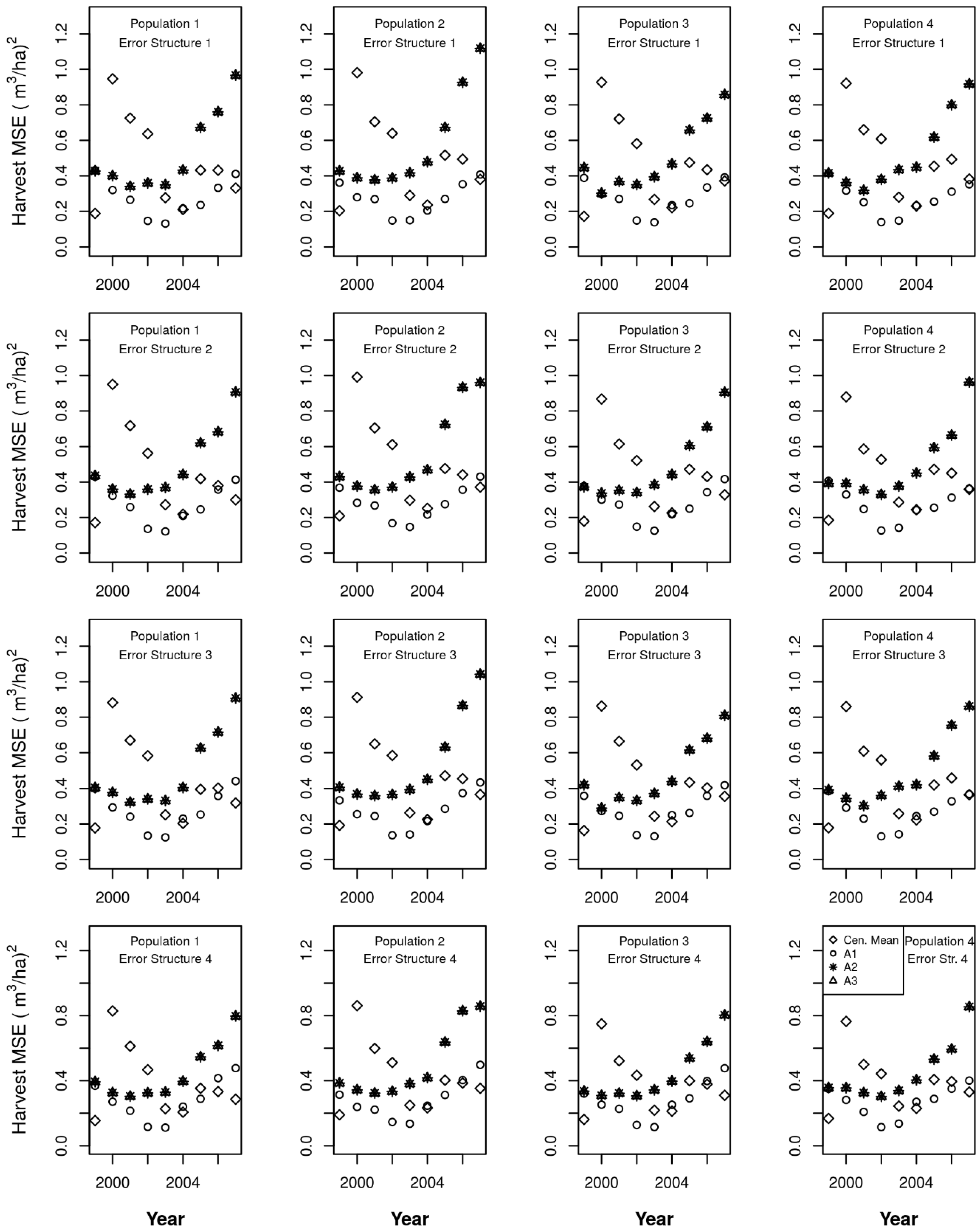
Similarly, a weighting variant is used here to incorporate the remotely sensed information on the timing of harvests, and the corresponding allocation of the other components of change, within a remeasurement window. For comparison, a centralized mean estimator for harvest is used in which the weight is split evenly between the center two years of the observation interval for each plot.

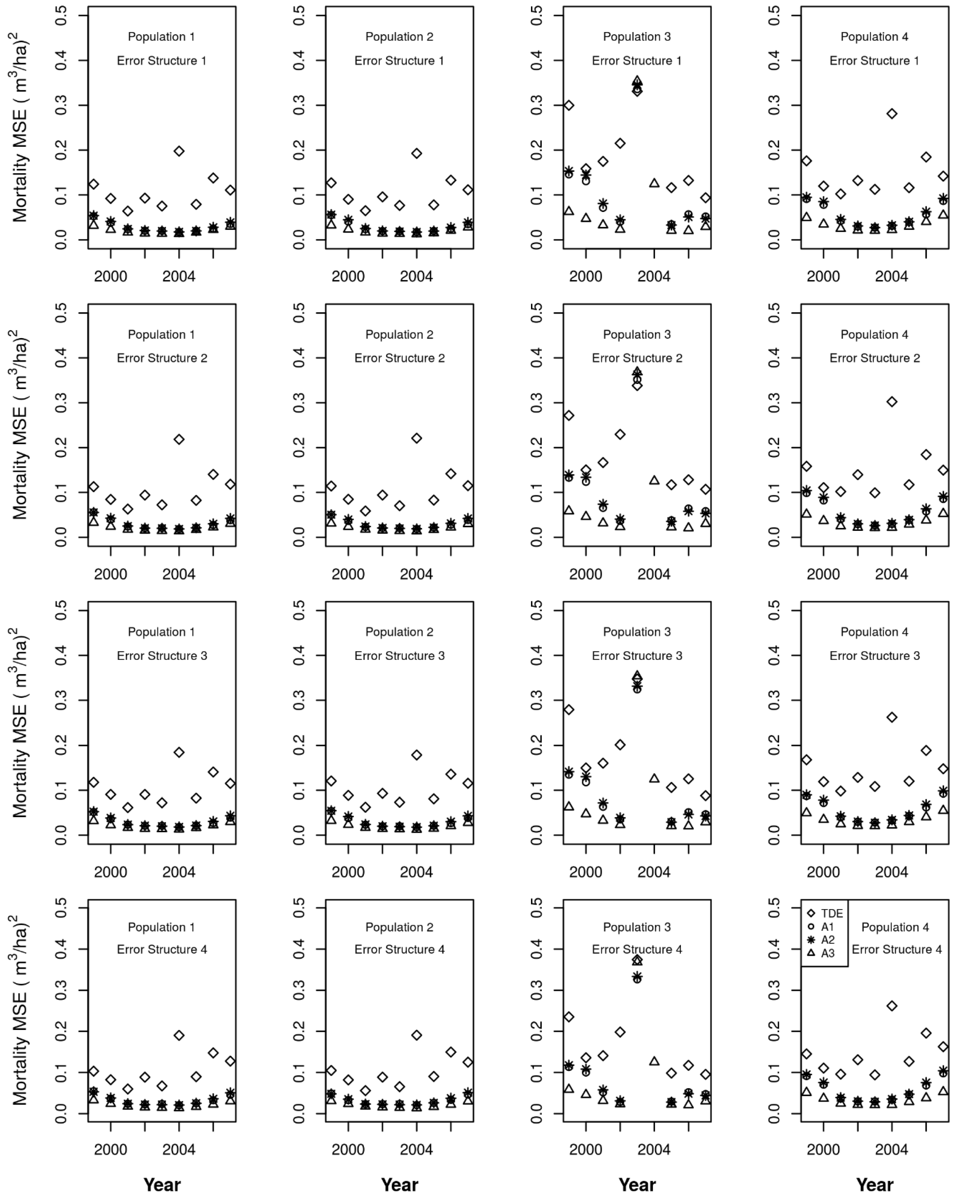
I compared three different levels of information that might be available from ICE observations, along with their related assumptions. In availability level 1 (A1), an ICE observation is made every two years and clearcuts are successfully identified 97.5% of the time, and there are no false positives. Other harvests are not identified by the ICE observation. Under this availability level, when a clearcut is identified, it is known to have occurred since the last plot visit, but may have been missed during intervening ICE observations.

Under availability level 2 (A2) an ICE observation is made every two years and every harvest (whether a partial harvest or a full harvest) is identified and assigned to the correct year, and there are no false positives. Also assume that proportional growth occurred before and after ICE harvest observations.

Availability level 3 (A3) reflects the same level of reliability as A2 with respect to harvest for ICE observations in which an ICE observation is made every two years and every harvest (whether a partial harvest or a full harvest) is identified and assigned to the correct year, and there are no false positives. Additionally, the ICE observations provide the same level of information on mortality, that is, all mortality trees can be identified, and there are no false positives.

Therefore, under availability level 1, I simplify the annual allocation problem by assuming that all observed growth occurred before the ICE clearcut observation. Under availability levels 2 and 3, for all harvests, I use an allocation that separates pre-harvest and post-harvest change based on an estimate of the proportion of volume harvested.

Each of these availability levels requires, at a minimum, the definition of two sets of weights, one set for the harvest component and the other for the remaining growth components. Additionally, each growth component could be assigned a unique set of weights if any auxiliary information contains enough detail.

Let ${\mathsf{\pi }}_{\mathit{i}\mathbf{,}\mathit{t}}^{\mathit{h}\mathsf{\alpha }}$ represent the weight for the harvest component under availability level α, for plot i and year t. (Naturally, the weight is equal to zero outside of the remeasurement interval.) Then, for each year in the estimation interval:

$${\mathit{h}}_{\mathit{i}\mathbf{,}\mathit{t}}^{\mathit{h}\mathsf{\alpha }}={\mathsf{\pi }}_{\mathit{i}\mathbf{,}\mathit{t}}^{\mathit{h}\mathsf{\alpha }}{\mathit{h}}_{\mathit{i}},$$

(6)

where h_i is the observation of cubic meter harvested volume on plot i during the remeasurement interval. The estimator for the harvest component for year t under availability level α is:

$${\mathit{C}}_{\mathit{t}}^{\mathit{h}\mathsf{\alpha }}=\frac{\mathbf{1}}{{\mathit{n}}_{\mathit{t}}}{\displaystyle \mathbf{\sum }_{\mathit{i}=\mathbf{1}}^{{\mathit{n}}_{\mathit{t}}}\frac{{\mathit{h}}_{\mathit{i}\mathbf{,}\mathit{t}}^{\mathit{h}\mathsf{\alpha }}}{{\mathit{p}}_{\mathit{i}\mathbf{,}\mathit{t}}}}$$

(7)

Weights must also be defined for the other components of change (live growth, entry, and mortality), to allocate the contribution to each year between the plot observation and the ICE-observed harvest. In simple cases, let ${\mathsf{\pi }}_{\mathit{i}\mathbf{,}\mathit{t}}^{\mathit{o}\mathsf{\alpha }}$ represent the weight defined for the other change components. The allocation for these other components of change on plot i for year t under α can be represented as:

$${\mathit{o}}_{\mathit{i}\mathbf{,}\mathit{t}}^{\mathit{o}\mathsf{\alpha }}={\mathsf{\pi }}_{\mathit{i}\mathbf{,}\mathit{t}}^{\mathit{o}\mathsf{\alpha }}{\mathit{o}}_{\mathit{i}},$$

(8)

where o_i is the observation of a specific component o for plot i during the interval. The estimator for the other components of change for year t under α is:

$${\mathit{C}}_{\mathit{t}}^{\mathit{o}\mathsf{\alpha }}=\frac{\mathbf{1}}{{\mathit{n}}_{\mathit{t}}}{\displaystyle \mathbf{\sum }_{\mathit{i}\mathbf{=}\mathbf{1}}^{{\mathit{n}}_{\mathit{t}}}\frac{{\mathit{o}}_{\mathit{i}\mathbf{,}\mathit{t}}^{\mathit{o}\mathsf{\alpha }}}{{\mathit{p}}_{\mathit{i}\mathbf{,}\mathit{t}}}}$$

(9)

2.3.1. Estimation of the Weights under α = A1:

Under the information availability of ICE observations of A1, when a clearcut is identified, it is known to have occurred since the last plot observation, but may have been missed during intervening ICE observations. To establish weights, I use the estimate of the probability of having missed the clearcut at previous ICE observations. Below, I use the fact that under this scenario, ICE data collected every two years will be in sync with about half of the plot observations collected under the panel design and out of sync with the other half, i.e. the first ICE observation after the plot observation will be in one year for half of the plots, and in two years for the other half of the plots.

I define $y_{i,I}$ as the number of years of the first ICE observation of clearcut for plot i since the previous plot measurement. Although it would be a rare event, I also define $y_{i,II}\ge y_{i,I}+2$ as the year of the second ICE observation of clearcut for plot i during the remeasurement interval, in order to estimate the weight for harvest. Additionally, when there are two ICE-identified clearcuts on plot i, I define r_i,I as the proportion of total clearcut volume in the first clearcut, and r_i,II = 1 − r_i,I as the proportion of total clearcut volume in the second clearcut. For α = A1:

$${\mathbf{\pi }}_{\mathit{i}\mathbf{,}\mathit{y}}^{\mathit{h}\mathit{A}\mathbf{1}}=\{\begin{array}{cc}{\mathbf{\pi }}_{\mathit{y}}\hfill & \mathrm{if}\mathrm{no}\mathrm{ICE}-\mathrm{identified}\mathrm{clearcut}\hfill \\ {{\mathit{y}}_{\mathit{i}\mathbf{,}\mathit{I}}}^{\mathbf{-}\mathbf{1}}\hfill & \mathrm{if}\mathrm{one}\mathrm{ICE}-\mathrm{identified}\mathrm{clearcut}\mathrm{and}\mathit{y}\mathbf{\le }{\mathit{y}}_{\mathit{i}\mathbf{,}\mathit{I}}\hfill \\ {\mathit{r}}_{\mathit{i}\mathbf{,}\mathit{I}}\hfill & \mathrm{if}\mathrm{ICE}\mathrm{is}\mathrm{out}\mathrm{of}\mathrm{sync}\mathrm{with}\mathrm{two}\mathrm{identified}\mathrm{clearcuts}\mathrm{and}\mathit{y}={\mathit{y}}_{\mathit{i}\mathbf{,}\mathit{I}}\hfill \\ \mathbf{.5}{\mathit{r}}_{\mathit{i}\mathbf{,}\mathit{I}}\hfill & \mathrm{if}\mathrm{ICE}\mathrm{is}\mathrm{in}\mathrm{sync}\mathrm{with}\mathrm{two}\mathrm{identified}\mathrm{clearcuts}\mathrm{and}\mathit{y}={\mathit{y}}_{\mathit{i}\mathbf{,}\mathit{I}}-\mathbf{1}\hfill \\ \mathbf{.5}{\mathit{r}}_{\mathit{i}\mathbf{,}\mathit{I}}\hfill & \mathrm{if}\mathrm{ICE}\mathrm{is}\mathrm{in}\mathrm{sync}\mathrm{with}\mathrm{two}\mathrm{identified}\mathrm{clearcuts}\mathrm{and}\mathit{y}={\mathit{y}}_{\mathit{i}\mathbf{,}\mathit{I}}\hfill \\ \mathbf{.5}{\mathit{r}}_{\mathit{i}\mathbf{,}\mathit{I}\mathit{I}}\hfill & \mathrm{if}\mathrm{two}\mathrm{ICE}-\mathrm{identified}\mathrm{clearcuts}\mathrm{and}\mathit{y}={\mathit{y}}_{\mathit{i}\mathbf{,}\mathit{I}\mathit{I}}-\mathbf{1}\hfill \\ \mathbf{.5}{\mathit{r}}_{\mathit{i}\mathbf{,}\mathit{I}\mathit{I}}\hfill & \mathrm{if}\mathrm{two}\mathrm{ICE}-\mathrm{identified}\mathrm{clearcuts}\mathrm{and}\mathit{y}={\mathit{y}}_{\mathit{i}\mathbf{,}\mathit{I}\mathit{I}}\hfill \\ 0\hfill & \mathrm{otherwise}\hfill \end{array}$$

(10)

The proportion r_i,I would have to be estimated. An estimate might be obtained from the ICE data but it is not directly available from the sample plot data. Under A1, I do not assume that one can confidently estimate r_i,I from the images, so I set it equal to 0.5, before expanding to the estimation interval:

$${\mathbf{\pi }}_{\mathit{i}\mathbf{,}\mathit{t}}^{\mathit{h}\mathit{A}\mathbf{1}}=\{\begin{array}{cc}{\mathbf{\pi }}_{\mathit{i}\mathbf{,}\mathit{y}}^{\mathit{h}\mathit{A}\mathbf{1}}& \mathrm{for}\mathit{t}\mathrm{within}\mathit{y}\hfill \\ \mathbf{0}& \mathrm{otherwise}\hfill \end{array}.$$

(11)

For the other components of change (live growth, entry, and mortality), the allocation to each year between plot observation and ICE-observed clearcut are as follows:

$${\mathbf{\pi }}_{\mathit{i}\mathbf{,}\mathit{y}}^{\mathit{o}\mathit{A}\mathbf{1}}=\{\begin{array}{ll}{\mathbf{\pi }}_{\mathit{y}}\hfill & \mathrm{if}\mathrm{no}\mathrm{ICE}-\mathrm{identified}\mathrm{clearcut}\hfill \\ {{\mathit{y}}_{\mathit{i}\mathbf{,}\mathit{I}}}^{-\mathbf{1}}\hfill & \mathrm{if}\mathrm{one}\mathrm{ICE}-\mathrm{identified}\mathrm{clearcut}\mathrm{and}\mathit{y}\mathbf{\le }{\mathit{y}}_{\mathit{i}\mathbf{,}\mathit{I}}\hfill \\ \mathbf{0}\hfill & \mathrm{if}\mathrm{one}\mathrm{ICE}-\mathrm{identified}\mathrm{clearcut}\mathrm{and}\mathit{y}\mathbf{>}{\mathit{y}}_{\mathit{i}\mathbf{,}\mathit{I}}\hfill \\ {\mathbf{\pi }}_{\mathit{y}}\hfill & \mathrm{if}\mathrm{two}\mathrm{or}\mathrm{more}\mathrm{ICE}-\mathrm{identified}\mathrm{clearcuts}\hfill \end{array}$$

(12)

Again, placing the weights within the estimation interval:

$${\mathbf{\pi }}_{\mathit{i}\mathbf{,}\mathit{t}}^{\mathit{o}\mathit{A}\mathbf{1}}=\{\begin{array}{cc}{\mathbf{\pi }}_{\mathit{i}\mathbf{,}\mathit{y}}^{\mathit{o}\mathit{A}\mathbf{1}}& \mathrm{for}\mathit{t}\mathrm{within}\mathit{y}\hfill \\ \mathbf{0}& \mathrm{otherwise}\hfill \end{array}.$$

(13)

2.3.2. Estimation of the Weights under α = A2:

Under availability level 2 (A2), I assume that I know if any harvest has occurred within the past two years and which year the harvest occurred. I further assume that I can estimate the proportion harvested to within ±5% (truncated at 0% and 100%), and proportional growth occurred before and after ICE harvest observations. Let ${\mathbf{\pi }}_{\mathit{i}\mathbf{,}\mathit{y}}^{\mathit{h}}$ be the ICE-estimated proportion of volume harvested in year y on plot i. Then the weight for the harvest component under α = A2 is:

$${\mathbf{\pi }}_{\mathit{i}\mathbf{,}\mathit{y}}^{\mathit{h}\mathit{A}\mathbf{2}}=\{\begin{array}{ll}{\mathbf{\pi }}_{\mathit{y}}\hfill & \mathrm{if}\mathrm{no}\mathrm{ICE}-\mathrm{identified}\mathrm{harvest}\mathrm{in}\mathrm{observation}\mathrm{interval}\hfill \\ {\mathbf{\pi }}_{\mathit{i}\mathbf{,}\mathit{y}}^{\mathit{h}}\hfill & \mathrm{if}\mathrm{ICE}-\mathrm{identified}\mathrm{harvest}\mathrm{in}\mathrm{year}\mathit{y}\hfill \\ 0\hfill & \mathrm{otherwise}\hfill \end{array}$$

(14)

As above, the expansion to the entire estimation interval is:

$${\mathbf{\pi }}_{\mathit{i}\mathbf{,}\mathit{t}}^{\mathit{h}\mathit{A}\mathbf{2}}=\{\begin{array}{cc}{\mathbf{\pi }}_{\mathit{i}\mathbf{,}\mathit{y}}^{\mathit{h}\mathit{A}\mathbf{2}}& \mathrm{for}\mathit{t}\mathrm{within}\mathit{y}\hfill \\ \mathbf{0}& \mathrm{otherwise}\hfill \end{array}.$$

(15)

To determine the allocation for the other components of change, let ${\mathbf{\pi }}_{\mathit{i}\mathbf{,}\mathit{F}}^{\mathit{h}}$ be the first (in year F, y_F) ICE-estimated proportion of volume harvested on plot i, and ${\mathbf{\pi }}_{\mathit{i}\mathbf{,}\mathit{S}}^{\mathit{h}}$ be the second (in year S, y_S) ICE-estimated harvest proportion on plot i. I set ${\mathbf{\pi }}_{\mathit{i}\mathbf{,}\mathit{F}}^{\mathit{h}}=\mathbf{0}$ if there is not an ICE-identified harvest during the interval, and I set ${\mathbf{\pi }}_{\mathit{i}\mathbf{,}\mathit{S}}^{\mathit{h}}=\mathbf{0}$ if there are not two ICE-identified harvests during the interval. The proportion remaining following the first harvest on plot i is ${\mathbf{\pi }}_{\mathit{i}\mathbf{,}\mathit{F}}^{\mathit{R}}=\mathbf{1}-{\mathbf{\pi }}_{\mathit{i}\mathbf{,}\mathit{F}}^{\mathit{h}}$. Likewise, the proportion remaining following the second harvest on plot i is ${\mathbf{\pi }}_{\mathit{i}\mathbf{,}\mathit{S}}^{\mathit{R}}=\mathbf{1}-{\mathbf{\pi }}_{\mathit{i}\mathbf{,}\mathit{S}}^{\mathit{h}}$. I calculate the annual allocation in three parts:

$${\mathit{a}}_{\mathit{y}}=\{\begin{array}{cc}\mathbf{\left(}{\mathbf{\pi }}_{\mathit{i}\mathbf{,}\mathit{F}}^{\mathit{h}}{\mathbf{\pi }}_{\mathit{y}}\mathbf{\right)}/{\displaystyle \mathbf{\sum }_{\mathit{y}\mathbf{=}\mathbf{1}}^{{\mathit{y}}_{\mathit{F}}}{\mathbf{\pi }}_{\mathit{y}}}& \mathrm{if}\mathrm{one}\mathrm{or}\mathrm{two}\mathrm{ICE}-\mathrm{identified}\mathrm{harvests}\mathrm{and}\mathit{y}\mathbf{\le }{\mathit{y}}_{\mathit{F}}\\ \mathbf{0}& \mathrm{otherwise}\end{array},$$

(16)

$${\mathit{b}}_{\mathit{y}}=\mathbf{\{}\begin{array}{cc}\mathbf{\left(}{\mathbf{\pi }}_{\mathit{i}\mathbf{,}\mathit{F}}^{\mathit{R}}{\mathbf{\pi }}_{\mathit{i}\mathbf{,}\mathit{S}}^{\mathit{h}}{\mathbf{\pi }}_{\mathit{y}}\mathbf{\right)}/{\displaystyle \mathbf{\sum }_{\mathit{y}\mathbf{=}\mathbf{1}}^{{\mathit{y}}_{\mathit{S}}}{\mathbf{\pi }}_{\mathit{y}}}& \mathrm{if}\mathrm{two}\mathrm{ICE}-\mathrm{identified}\mathrm{harvests}\mathrm{and}\mathit{y}\mathbf{\le }{\mathit{y}}_{\mathit{S}}\\ \mathbf{0}& \mathrm{otherwise}\end{array},$$

(17)

and

$${\mathit{c}}_{\mathit{y}}=\mathbf{\left(}{\mathbf{\pi }}_{\mathit{i}\mathbf{,}\mathit{F}}^{\mathit{R}}{\mathbf{\pi }}_{\mathit{i}\mathbf{,}\mathit{S}}^{\mathit{R}}{\mathbf{\pi }}_{\mathit{y}}\mathbf{\right)}.$$

(18)

Summing the parts results in the annual proportion:

$${\mathbf{\pi }}_{\mathit{i}\mathbf{,}\mathit{y}}^{\mathit{o}\mathit{A}\mathbf{2}}={\mathit{a}}_{\mathit{y}}\mathbf{+}{\mathit{b}}_{\mathit{y}}\mathbf{+}{\mathit{c}}_{\mathit{y}}.$$

(19)

And, again, the weights within the estimation interval are:

$${\mathbf{\pi }}_{\mathit{i}\mathbf{,}\mathit{t}}^{\mathit{o}\mathit{A}\mathbf{2}}=\{\begin{array}{cc}{\mathbf{\pi }}_{\mathit{i}\mathbf{,}\mathit{y}}^{\mathit{o}\mathit{A}\mathbf{2}}& \mathrm{for}\mathit{t}\mathrm{within}\mathit{y}\hfill \\ \mathbf{0}& \mathrm{otherwise}\hfill \end{array}.$$

(20)

2.3.3. Estimation of the Weights under α = A3:

Under availability level 3 (A3), the information available for harvest estimates is exactly the same as under A2 above and the same assumptions are used. The weight for the harvest component under α = A3 is:

$${\mathbf{\pi }}_{\mathit{i}\mathbf{,}\mathit{y}}^{\mathit{h}\mathit{A}\mathbf{3}}=\{\begin{array}{ll}{\mathbf{\pi }}_{\mathit{y}}\hfill & \mathrm{if}\mathrm{no}\mathrm{ICE}-\mathrm{identified}\mathrm{harvest}\mathrm{in}\mathrm{observation}\mathrm{interval}\hfill \\ {\mathbf{\pi }}_{\mathit{i}\mathbf{,}\mathit{y}}^{\mathit{h}}\hfill & \mathrm{if}\mathrm{ICE}-\mathrm{identified}\mathrm{harvest}\mathrm{in}\mathrm{year}\mathit{y}\hfill \\ 0\hfill & \mathrm{otherwise}\hfill \end{array}.$$

(21)

$${\mathbf{\pi }}_{\mathit{i}\mathbf{,}\mathit{t}}^{\mathit{h}\mathit{A}\mathbf{3}}=\{\begin{array}{cc}{\mathbf{\pi }}_{\mathit{i}\mathbf{,}\mathit{y}}^{\mathit{h}\mathit{A}\mathbf{3}}& \mathrm{for}\mathit{t}\mathrm{within}\mathit{y}\hfill \\ \mathbf{0}& \mathrm{otherwise}\hfill \end{array}.$$

(22)

Availability level A3 also provides information for mortality estimates that can be used in the same way as the harvest information is used above. The weight for the mortality component under α = A3 is:

$${\mathbf{\pi }}_{\mathit{i}\mathbf{,}\mathit{y}}^{\mathit{m}\mathit{A}\mathbf{3}}=\{\begin{array}{ll}{\mathbf{\pi }}_{\mathit{y}}\hfill & \mathrm{if}\mathrm{no}\mathrm{ICE}-\mathrm{identified}\mathrm{mortality}\mathrm{in}\mathrm{observation}\mathrm{interval}\hfill \\ {\mathbf{\pi }}_{\mathit{i}\mathbf{,}\mathit{y}}^{\mathit{m}}\hfill & \mathrm{if}\mathrm{ICE}-\mathrm{identified}\mathrm{mortality}\mathrm{in}\mathrm{year}\mathit{y}\hfill \\ 0\hfill & \mathrm{otherwise}\hfill \end{array}.$$

(23)

$${\mathbf{\pi }}_{\mathit{i}\mathbf{,}\mathit{t}}^{\mathit{m}\mathit{A}\mathbf{3}}=\{\begin{array}{cc}{\mathbf{\pi }}_{\mathit{i}\mathbf{,}\mathit{y}}^{\mathit{m}\mathit{A}\mathbf{3}}& \mathrm{for}\mathit{t}\mathrm{within}\mathit{y}\hfill \\ \mathbf{0}& \mathrm{otherwise}\hfill \end{array}.$$

(24)

There is room for debate as to whether one should attempt to further adjust the components of entry and live growth due to this additional information on mortality. After all, the timing of mortality does affect both of these components. On the one hand, all forested populations have constant mortality, and it would seem that no modeled temporal adjustment in the other components would be helpful for this type of mortality. On the other hand, large mortality events do sometimes occur, leading to a loss of volume equivalent to that of some harvesting systems. In fact, one such event was built into Population 3 in this study. Because mortality is usually more consistently distributed throughout the population, I do not attempt to adjust the remaining components relative to observations of “normal” mortality, arbitrarily defined as those that are estimated to be less than one-half of the standing volume. I do adjust the remaining components relative to observations of mortality that are estimated to be greater than or equal to one-half of the standing volume in the same way that I adjusted those components relative to observations for harvest above. That is, to determine the allocation for these two other components of change, let ${\mathbf{\pi }}_{\mathit{i}\mathbf{,}\mathit{F}}^{\mathit{h}\mathit{m}}$ be the first (in year F, y_F) ICE-estimated proportion of volume harvested or proportion dying that is greater than half of the standing volume (hereafter referred to as a large mortality event) on plot i, and ${\mathbf{\pi }}_{\mathit{i}\mathbf{,}\mathit{S}}^{\mathit{h}\mathit{m}}$ be the second (in year S, y_S) ICE-estimated harvest proportion or proportion of the standing volume lost during a large mortality event on plot i. I set ${\mathbf{\pi }}_{\mathit{i}\mathbf{,}\mathit{F}}^{\mathit{h}\mathit{m}}=\mathbf{0}$ if there is no harvest or large mortality event during the interval, and I set ${\mathbf{\pi }}_{\mathit{i}\mathbf{,}\mathit{S}}^{\mathit{h}\mathit{m}}=\mathbf{0}$ if there are no two such events during the interval. The proportion remaining following the first event on plot i is ${\mathbf{\pi }}_{\mathit{i}\mathbf{,}\mathit{F}}^{\mathit{R}}=\mathbf{1}-{\mathbf{\pi }}_{\mathit{i}\mathbf{,}\mathit{F}}^{\mathit{h}\mathit{m}}$. Likewise, the proportion remaining following the second event on plot i is ${\mathbf{\pi }}_{\mathit{i}\mathbf{,}\mathit{S}}^{\mathit{R}}=\mathbf{1}-{\mathbf{\pi }}_{\mathit{i}\mathbf{,}\mathit{S}}^{\mathit{h}\mathit{m}}$. The same as for A2 above, I calculate the annual allocation in three parts:

$${\mathit{a}}_{\mathit{y}}=\{\begin{array}{cc}\mathbf{\left(}{\mathbf{\pi }}_{\mathit{i}\mathbf{,}\mathit{F}}^{\mathit{h}\mathit{m}}{\mathbf{\pi }}_{\mathit{y}}\mathbf{\right)}/{\displaystyle \mathbf{\sum }_{\mathit{y}\mathbf{=}\mathbf{1}}^{{\mathit{y}}_{\mathit{F}}}{\mathbf{\pi }}_{\mathit{y}}}& \mathrm{if}\mathrm{one}\mathrm{or}\mathrm{two}\mathrm{ICE}-\mathrm{identified}\mathrm{events}\mathrm{and}\mathit{y}\mathbf{\le }{\mathit{y}}_{\mathit{F}}\\ \mathbf{0}& \mathrm{otherwise}\end{array},$$

(25)

$${\mathit{b}}_{\mathit{y}}=\{\begin{array}{cc}\mathbf{\left(}{\mathbf{\pi }}_{\mathit{i}\mathbf{,}\mathit{F}}^{\mathit{R}}{\mathbf{\pi }}_{\mathit{i}\mathbf{,}\mathit{S}}^{\mathit{h}\mathit{m}}{\mathbf{\pi }}_{\mathit{y}}\mathbf{\right)}/{\displaystyle \mathbf{\sum }_{\mathit{y}\mathbf{=}\mathbf{1}}^{{\mathit{y}}_{\mathit{S}}}{\mathbf{\pi }}_y}& \mathrm{if}\mathrm{two}\mathrm{ICE}-\mathrm{identified}\mathrm{events}\mathrm{and}\mathit{y}\mathbf{\le }{\mathit{y}}_{\mathit{S}}\\ 0& \mathrm{otherwise}\end{array},$$

(26)

and

$${\mathit{c}}_{\mathit{y}}=\mathbf{\left(}{\mathbf{\pi }}_{\mathit{i}\mathbf{,}\mathit{F}}^{\mathit{R}}{\mathbf{\pi }}_{\mathit{i}\mathbf{,}\mathit{S}}^{\mathit{R}}{\mathbf{\pi }}_{\mathit{y}}\mathbf{\right)}.$$

(27)

Summing the parts results in the annual proportion:

$${\mathbf{\pi }}_{\mathit{i}\mathbf{,}\mathit{y}}^{\mathit{o}\mathit{A}\mathbf{3}}={\mathit{a}}_{\mathit{y}}\mathbf{+}{\mathit{b}}_{\mathit{y}}\mathbf{+}{\mathit{c}}_{\mathit{y}}.$$

(28)

And, again, the weights within the estimation interval are:

$${\mathbf{\pi }}_{\mathit{i}\mathbf{,}\mathit{t}}^{\mathit{o}\mathit{A}\mathbf{3}}=\{\begin{array}{cc}{\mathbf{\pi }}_{\mathit{i}\mathbf{,}\mathit{y}}^{\mathit{o}\mathit{A}\mathbf{3}}& \mathrm{for}\mathit{t}\mathrm{within}\mathit{y}\hfill \\ \mathbf{0}& \mathrm{otherwise}\hfill \end{array}.$$

(29)

2.4. Estimation of Initial Annual Volume

The class of plot sample designs being discussed here provides high variance, single-panel direct annual estimates of standing volume. Compatible annual systems require estimates of standing volume at a particular time of year, and here I have defined that time to be the beginning of the year, or prior to the growing season. Here, as in Roesch et al. [1], in order to ensure compatibility, I use recursive estimation to estimate initial annual volume and denote the series as ${\widehat{Y}}^{\mathit{R}}$. The reader interested in the details of the recursive estimation approach is referred to the previous work, or as an exercise, can derive the recursive series from Equation (1) above. Note that it is important to carefully consider the start point for any recursive series of estimates because all of the other estimates are based on it. In this study, I used the mean of nine panel mean, corresponding to years 1999 to 2007, to estimate the initial volume for the central year (2003), as a start point for each recursive series.

2.5. Estimation Systems

The estimators described above can be combined to define various estimation systems. Also, the noise in successive annual estimates can be reduced by using a filter to combine the information from successive observations. One common filter is known as the moving window estimator. In general, a moving window estimator for time t, of size s (an odd positive integer) is:

$${\mathsf{\epsilon }}_{\mathit{t}}^{\mathit{s}}={\displaystyle \mathbf{\sum }_{\mathit{j}\mathbf{=}\mathit{t}\mathbf{-}\mathbf{\left(}\mathbf{\left(}\mathit{s}\mathbf{-}\mathbf{1}\mathbf{\right)}\mathbf{/}\mathbf{2}\mathbf{\right)}}^{\mathit{t}\mathbf{+}\mathbf{\left(}\mathbf{\left(}\mathit{s}\mathbf{-}\mathbf{1}\mathbf{\right)}\mathbf{/}\mathbf{2}\mathbf{\right)}}{\mathsf{\epsilon }}_{\mathit{j}}}.$$

(30)

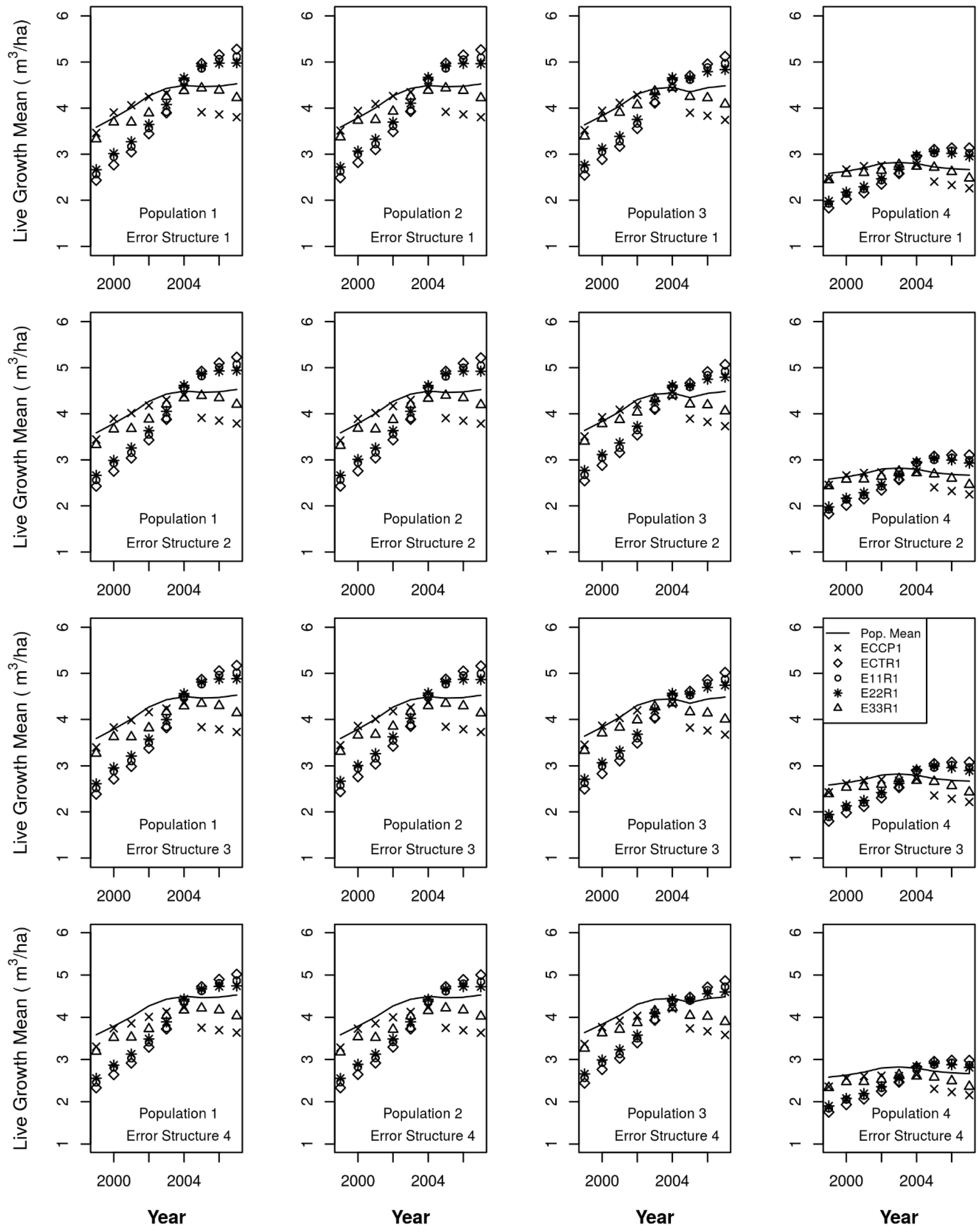
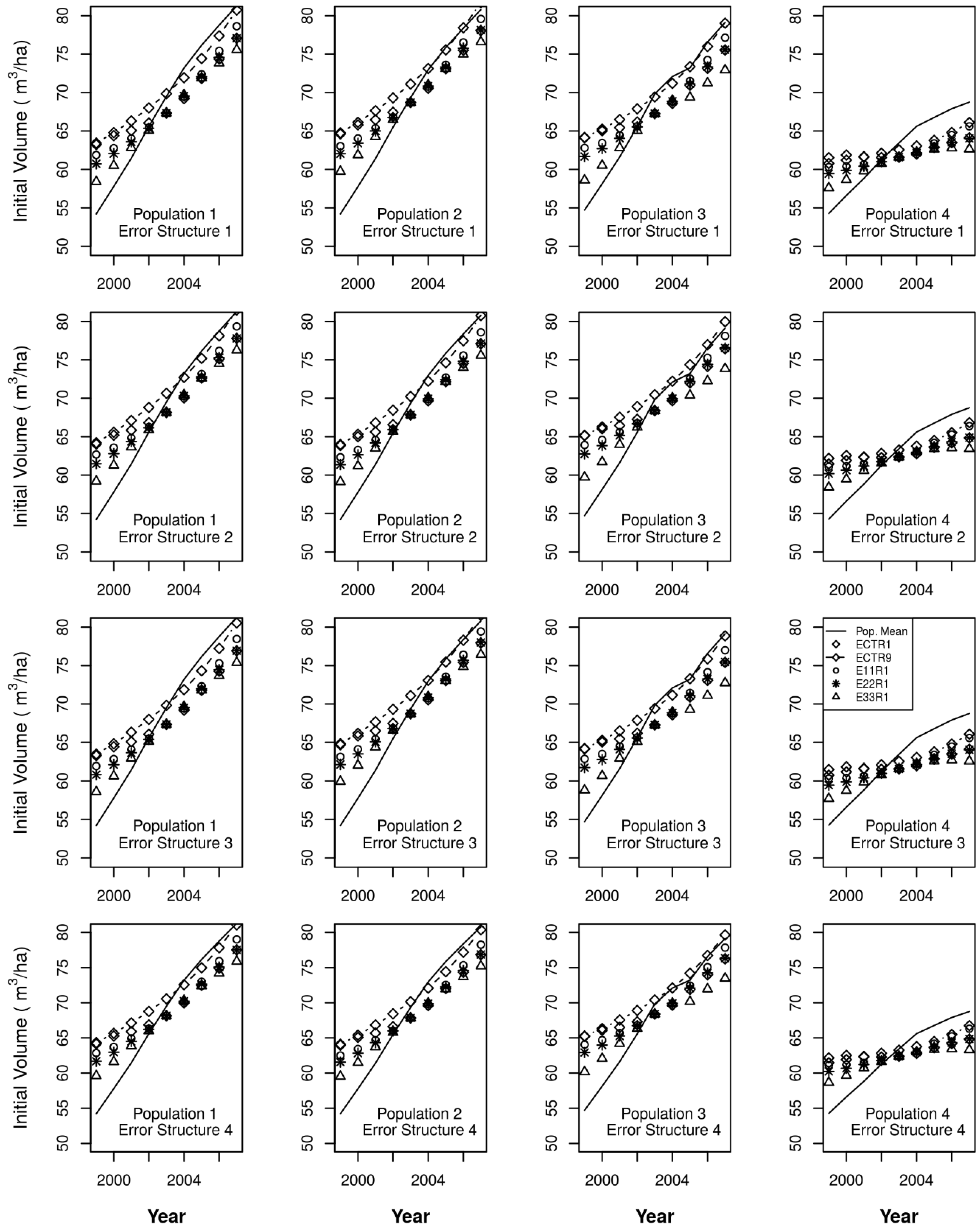
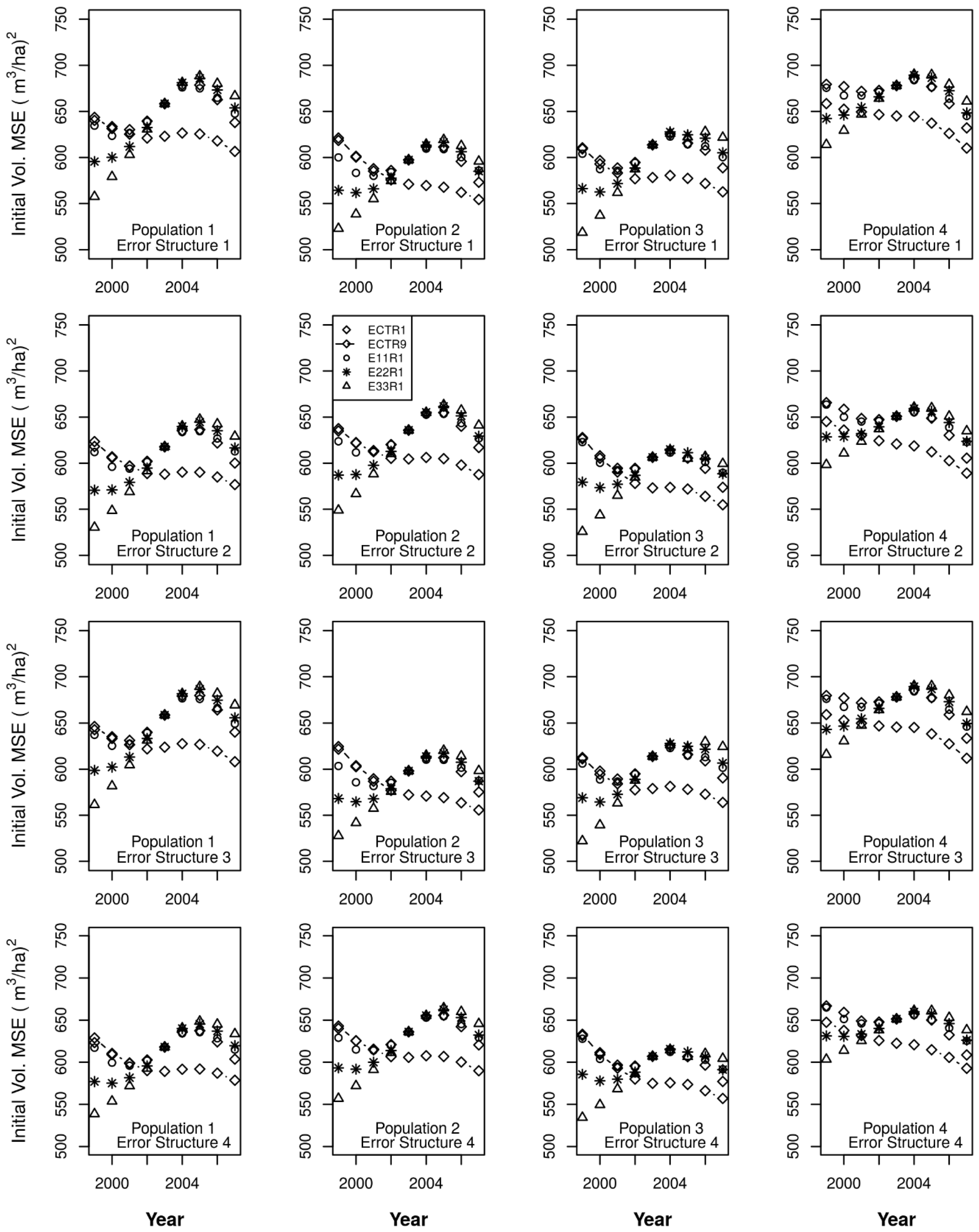
The estimation systems discussed here include:

ECCP1 = C^M for all components and for annual volume,

ECTR1 = C^M for harvest, C^T for the other change components, ${\widehat{Y}}^{\mathit{R}}$ for annual volume,

E11R1 = C^hA1 for harvest, C°^A1 for the other change components, ${\widehat{Y}}^{\mathit{R}}$ for annual volume,

E22R1 = C^hA2 for harvest, C°^A2 for the other change components, ${\widehat{Y}}^{\mathit{R}}$ for annual volume,

E33R1 = C^hA3 for harvest, C^mA3 for harvest, C°^A3 for the other change components,${\widehat{Y}}^{\mathit{R}}$ for annual volume,

ECTR9 = nine-year moving window on ECTR1.

2.6. Estimation System Evaluation

Estimator robustness was tested in a simulation by sampling the population under four different assumptions of sampling error structure for the plot data and three different availability levels of the remotely sensed data. As described above, each simulation consisted of 1000 iterations of 1000 plots each (without replacement) from the population. For each iterate, for each year, I calculated the empirical bias (EB) and the empirical mean squared error (MSE), over the 1000 iterations, between each estimator and the true population values under each of the four error structures. I use the empirical MSE as one criterion for judging the effectiveness of the external information. That is:

$$\mathit{M}\mathit{S}{\mathit{E}}_{\mathit{P}\mathit{E}\mathit{S}}=\frac{\mathbf{1}}{\mathbf{1000}}{\displaystyle \mathbf{\sum }_{\mathit{i}\mathbf{=}\mathbf{1}}^{\mathbf{1000}}{\mathbf{\left(}{\widehat{\mathit{x}}}_{\mathit{P}\mathit{E}{\mathit{S}}_{\mathit{i}}}-{\mathit{X}}_{\mathit{P}}\mathbf{\right)}}^{\mathbf{2}}},$$

(31)

where ${\widehat{\mathit{x}}}_{\mathit{P}\mathit{E}{\mathit{S}}_{\mathit{i}}}$ is the sample estimate of any variable, X, in population P for estimator E, under error structure S for iterate i.

3. Results

Figure 1 shows the means of five live growth estimators including the centralized mean, the trend-distributed estimator, and the ICE-enhanced estimators under availability levels A1, A2, and A3 relative to the population mean for live growth, over 1000 iterations of 1000 samples for each population and sample error structure. Note in this figure that the centralized mean estimator, which is model unbiased under a simple linear model, does show some bias in the later years of estimation. It is often the case that the population mean trend, which is usually unknown, will not conform to a simple linear model over a relatively long time span of interest. The ICE-enhanced estimators are shown to adjust this deviance from the trend line, although in most cases availability level 3 was necessary to show improvement in tracking the trend line.

The means of five entry estimators are shown in Figure 2, including the centralized mean, the trend-distributed estimator, and the three ICE-enhanced estimators under availability levels A1, A2, and A3 relative to the population mean for entry, over 1000 iterations of 1000 samples for each population and sample error structure. Of note in Figure 2 is that the results for entry in the later estimation years are very much the same as they were for live growth (in Figure 1); however, the ICE estimates in the earlier years appear to be slightly more biased.

Figure 3 gives the empirical means of the harvest estimators under A1, A2, and A3 and the centralized mean estimator relative to the population mean for harvest, over 1000 iterations of 1000 samples for each population and sample error structure for estimation years 1999 through 2007. Note that for harvest, A2 and A3 are identical, and therefore the estimators are indistinguishable in both Figure 3 and Figure 4, which gives the corresponding MSEs for the four estimators. Figure 3 shows that the ICE observations contribute to improved tracking of the mean harvest trend under A2 and A3 relative to both the centralized mean and A1, although a few of the annual estimates show slightly less bias for the centralized mean estimator. The MSE results in Figure 4 are less conclusive. The ICE-assisted estimators for harvest have lower MSEs in the earlier years of the estimation interval but the advantage does not appear to carry through to the later years. We see in both Figure 3 and Figure 4 that the general pattern or ranking of the annual estimators is fairly consistent through all populations and plot observation error structures.

In Figure 5, I show the MSEs of the mortality estimators over 1000 iterations of 1000 samples for each population and sample error structure. The reader may recall that population 3 was constructed with an introduced catastrophic mortality event in 2004. If the individual graphs in the figure were scaled identically to allow the display of all of the results, the results for all years except 2004 would be indistinguishable. Therefore, to enhance clarity, the three of the four estimators are not shown not shown for population 3, year 2004, the trend-distributed estimator and the estimators from A1 and A2, as their values were about 12 to 15 times higher than the value for A3. Except for population 3, the ICE-assisted estimators have lower MSEs than the unassisted trend-distributed estimator. In all populations, under all error structures, the A3 estimator has either the lowest MSEs throughout the estimation interval or is tied for the lowest.

The annual estimation of both mortality and harvest are notoriously difficult in large-area monitoring efforts using long (in this case ten-year) observation intervals. The design considered here does benefit from being temporally and spatially interpenetrating, but that interpenetration cannot fully compensate for the fact that the a series of decade-long intervals are being used in an attempt to form annual estimates. Growth on living trees including trees which die or are harvested during the observation interval is not observed by the ground plot design. The different levels of error structure introduced into this study take this interval estimation problem into account. Figure 6 and Figure 7 give the means and MSEs, respectively, for initial annual volume under the five estimation systems described in Section 2.5 for the four populations and four error structures. Figure 6 shows the deviances from the trend lines that might be expected as a result of the bias introduced in the error structures. It appears from the MSE plots in Figure 7 that the ICE-assisted estimators are superior in the early years of the estimation interval over all populations and error structures, while ECTR9 appears to prevail in the later years. Examination of Figure 6 suggests that the intentionally introduced (sampling) bias is simply overriding some of the benefits of the ICE information.

4. Discussion

Roesch et al. [1] showed one way to augment revisited plot observations with a temporal interval of ten years with image change estimates (ICE) observations every two years while the temporal dimension of the population of interest, and the estimands of interest, were fixed at one year. Here, I extend that investigation with alternative error structures and hierarchical assumptions of the availability of ICE-derived information. I show the interacting effects on estimation of increasing albeit realistic levels of sampling error and increasing levels of information from remotely sensed ICE estimates. In this investigation, estimator performance was tested in a simulation designed to consider a wide range of potential sampling and measurement errors. Within the simulation, I use four sampling error structures for the measured plot data and three levels of availability of the remotely sensed image change estimates. The errors that are simulated here would exist in most national forest inventories but would be largely unknown and are often ignored. Simulations that do not attempt to consider sampling and measurement errors do not give a realistic picture of estimator performance or advantage. As Eastaugh and Hasenauer [2] point out, and as shown here, plausible levels of sampling and measurement errors can profoundly affect what might otherwise be considered theoretically superior estimators.

5. Conclusions

While a clear benefit is shown to increasing knowledge on the timing of mortality and harvest events on the annual estimation of mortality, harvest, and live growth, improvement in the annual estimation of entry and initial volume was less consistently achieved. As a practical matter, it may be possible but certainly more difficult to use the ICE images to also enhance the estimation of the timing of entry, especially for forest plantations. This would be more difficult because the images would have to be used to not only observe new trees, but also to observe when new trees reach a defined size. Because of this practical difficulty, I did not add a fourth level of ICE availability to the simulations that included prediction of entry. If I had, that fourth level may have shown much better results with respect to annual estimation of both entry and initial volume; however, it is important in simulations to include parameter levels that one knows to be realistically achievable, for it is far too easy to preordain a favorable result. The simulations conducted here are realistic and do show the difficulty that exists when attempting to compensate for a sparsely informed sample. Large observation intervals tend to mask trends, even when those intervals overlap and are staggered annually as they are in the design investigated here.