Developing an Improved Parameter Estimation Method for the Segmented Taper Equation through Combination of Constrained Two-Dimensional Optimum Seeking and Least Square Regression

Abstract

The segmented taper equation has great flexibility and is widely applied in exiting taper systems. The unconstrained least square regression (ULSR) was generally used to estimate parameters in previous applications of the segmented taper equations. The joint point parameters estimated with ULSR may fall outside the feasible region, which leads to the results of the segmented taper equation being uncertain and meaningless. In this study, a combined method of constrained two-dimensional optimum seeking and least square regression (CTOS & LSR) was proposed as an improved method to estimate the parameters in the segmented taper equation. The CTOS & LSR was compared with ULSR for both individual tree-level equation and the population average-level equation using data from three tropical precious tree species (Castanopsis hystrix, Erythrophleum fordii, and Tectona grandis) in the southwest of China. The differences between CTOS & LSR and ULSR were found to be significant. The segmented taper equation estimated using CTOS & LSR resulted in not only increased prediction accuracy, but also guaranteed the parameter estimates in a more meaningful way. It is thus recommended that the combined method of constrained two-dimensional optimum seeking and least square regression should be a preferred choice for this application. The computation procedures required for this method is presented in the article.

1. Introduction

The mathematical function (or equation) describing the variation of the tree diameter at any point of the stem with the distance from the tree top is known as the stem taper equation [1]. Using this equation, one may calculate stem diameter at any arbitrary height and conversely, calculate tree height for any arbitrary stem diameter. Consequently, stem volume can be calculated for any log specification, and a volume equation can be developed for classified product dimensions [2]. In many countries, especially the United States and Canada, stem taper equations have been commonly used to replace volume tables and volume equations for estimating stem volume, merchantable volume ratio, 3-D reconstruction of stem and simulation, and optimization of bucking [3,4,5]. Therefore, developing a stem taper equation with high predictive precision has always been a matter of interest to forest managers and forest engineers as the taper equation provides technical support to forest management.

Numerous forms of the taper equation have been developed over the past century ranging from simple to complex. These taper equations can be divided into three categories: simple taper equation [1,6,7,8,9,10,11,12], segmented taper equation [13,14,15,16,17], and variable-exponent taper equation [3,18,19,20,21,22]. Simple taper equations are easy to fit, and can be used to calculate the stem volume applying the integration method. Relatively simple taper functions can effectively describe the general taper of the trees. However, they lack the ability to describe the entire stem accurately. They may provide reasonable estimates in a mid-portion of the stem, but usually are less accurate in estimating the profile in the butt or upper stem segments [3,13,18,23]. As compared to the simple taper equation, the segmented taper equation exhibits a higher precision of diameter estimation and also could be used to describe the entire stem profile more efficiently [13,24,25]. The variable-exponent taper equation also has a high estimation precision, but it cannot be used to estimate volume by integration without the aid of a computer program [3,17,26]. Overall, the segmented taper equation has greater flexibility than other taper equations and therefore has frequently been applied along with different modelling approaches (e.g., traditional least square regression, seemingly unrelated regression and nonlinear mixed-effects model) [14,17,24,25].

The Max and Burkhart [13] taper equation is one of the most typical segmented taper equations to describe tree stem taper [14,25,27]. This equation consists of three different quadratic functions joined at two joint points, and therefore is flexible enough to describe complex and irregular stem profiles. Many researchers have used this equation for the prediction of tree taper [15,17,24,25,28,29,30,31,32]. Two joint point (upper and lower) parameters (the feasible region of two parameters lies between 0 and 1) in the Max and Burkhart [13] taper equation were usually estimated by applying a traditional unconstrained least square regression (ULSR) method and subjective experience (SE) method [13,17,25,33]. However, in a practical application, it has been found that the estimates of the two joint point parameters obtained from ULSR sometimes fall outside the feasible region of the corresponding estimated parameters, which makes the results meaningless [34]. The study involved the application of a simplex method with constraint to estimate parameters of the Max and Burkhart [13] taper equation. However, this failed to converge and was found very slow computationally. In addition, the study also revealed that the estimates of the two joint point parameters obtained by ULSR varied with the starting values of the parameters. Therefore, the developed Max and Burkhart [13] taper equation based on ULSR is subject to a great uncertainty. The SE method has a great uncertainty in estimation of the join point parameters due to unpredictable man-induced factors and inevitable measurement errors [35]. These uncertainties directly influence the estimation precision and practicability of the taper equations.

The objective of this study was thus to propose a combined method of constrained two-dimensional optimum seeking and least square regression (CTOS & LSR) as an improved method to estimate parameters of the segmented taper equation based on Hua’s optimum seeking theory and golden section search approach [36]. The data from three tropical precious tree species Castanopsis hystrix Miq. (C. hystrix), Erythrophleum fordii Oliv. (E. fordii), and Tectona grandis L.F. (T. grandis) in southwest China were used to evaluate the methods. Also, CTOS & LSR was compared with the commonly used ULSR approach by means of developing the Max and Burkhart [13] taper equation at both individual tree-levels and population average-levels.

2. Materials and Methods

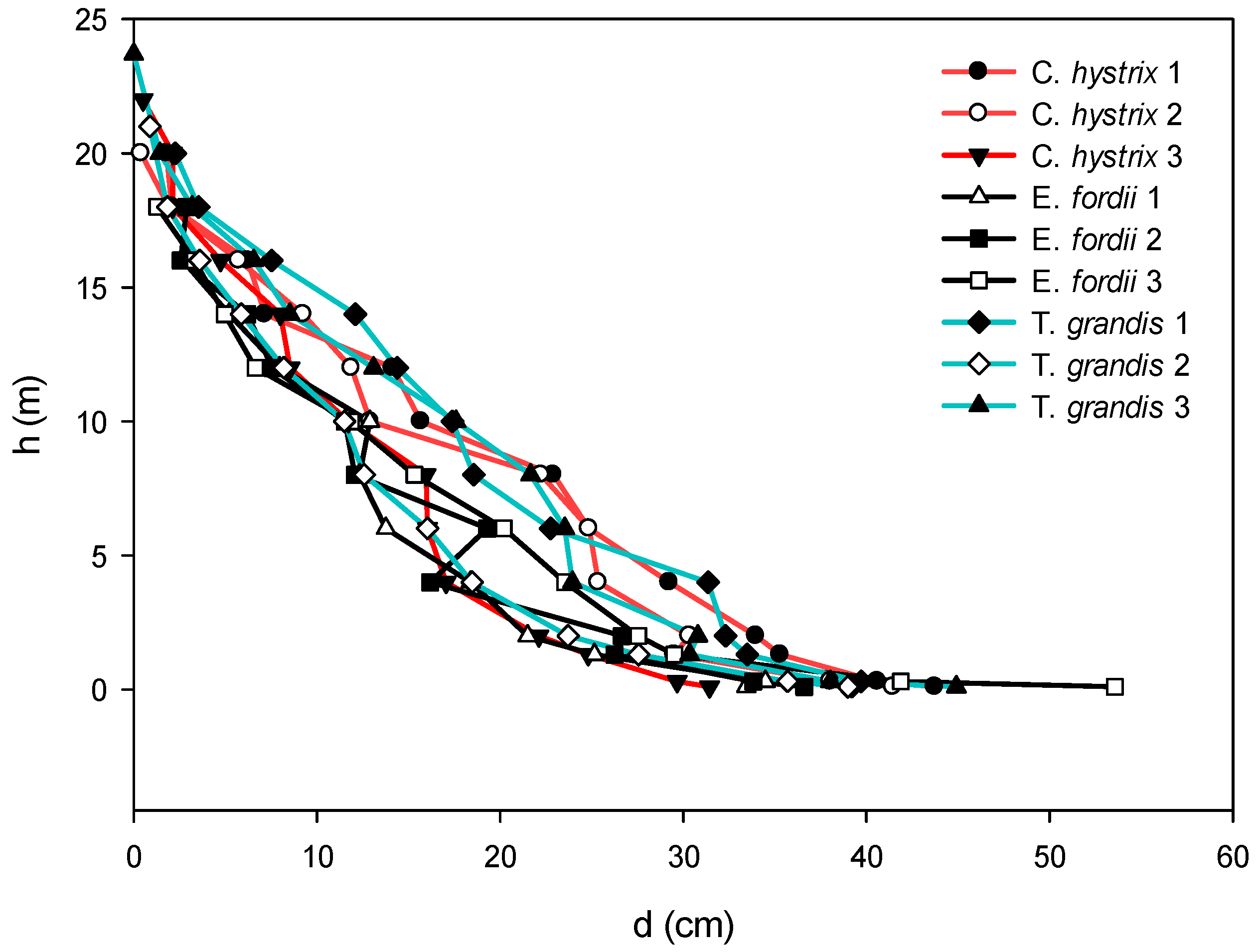
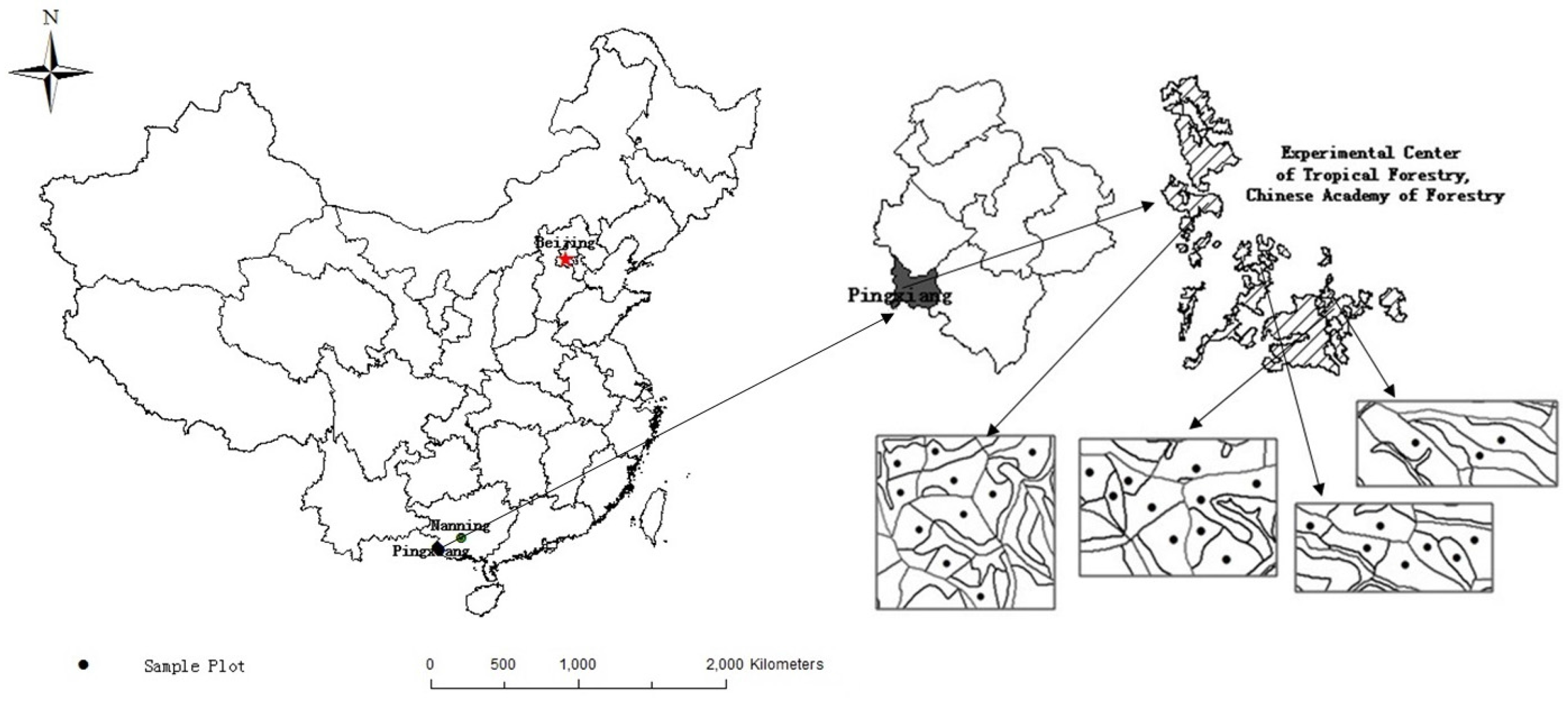
2.1. Data

We used data from a total of 30 square-shaped permanent sample plots (PSPs) established in 2014 across three pure even-aged C. hystrix, E. fordii, and T. grandis plantations (each tree species with 10 PSPs) located in the Experimental Center of Tropical Forestry, Chinese Academy of Forestry Sciences (Figure 1). C. hystrix, E. fordii, and T. grandis are tropical precious tree species in southern China. The data were collected by the Research Institute of Forest Resources Information Techniques, Chinese Academy of Forestry. Stands were selected on the basis of the following criteria: (1) pure species; (2) fully stocked; (3) even-aged; and (4) minimum or no disturbance. Sample plots were avoided near major roads because road construction might have altered soil drainage and affected tree growth. Once a stand was located, a 600 m² permanent sample plot was established. Four trees per sample plot, each representing dominant height, codominant height, average height, and suppressed height were selected. These trees were felled, and cross-sectional slices of stem (disks) were obtained from 0.33 m, 0.67 m, 1.3 m, and every 1.3 m interval thereafter until an outside bark diameter of 7.0 cm was reached. Disks were then taken every 20 cm between 7 cm and 4 cm outside bark diameter. Many tree characteristics such as outside bark diameter at breast height (D), total height (H), height to live crown base, and crown width, were measured for each sample tree. Summary statistics of D and H data are listed in

Table 1. Summary statistics of full dataset.

Tree Species	Variable	No.	Mean	Max	Min	SD	CV
C. hystrix	D (cm)	40	22.12	37.55	8.70	7.40	0.33
	H (m)	40	21.43	30.50	10.10	5.21	0.24
E. fordii	D (cm)	40	21.15	29.50	10.05	4.52	0.21
	H (m)	40	18.64	22.40	11.80	2.71	0.15
T. grandi	D (cm)	40	25.93	37.95	12.70	5.49	0.21
	H(m)	40	21.16	27.40	9.30	3.52	0.17

D, diameter at breast height; H, total tree height; SD, standard deviation; CV, coefficient of variation.

. We applied two approaches for fitting and testing the Max and Burkhart [13] taper equations; (i) at individual tree-level using sub-dataset of nine dominant and codominant trees (three trees from each tree species) (Figure 2); (ii) at population average-level using full dataset of 120 trees (Table 1).

2.2. Taper Equation

The Max and Burkhart [13] taper equation is:

$$y={\mathsf{\beta }}_1(x-1)+{\mathsf{\beta }}_2(x^2-1)+{\mathsf{\beta }}_3{({\mathsf{\alpha }}_1-x)}^2{I}_1+{\mathsf{\beta }}_4{({\mathsf{\alpha }}_2-x)}^2{I}_2+\mathsf{\epsilon }$$

(1)

where $y=d^2/D^2$, $x=h/H$, $h$ is the height above ground to measurement point (m), $d$ is the outside bark diameter at height $h$ above ground (cm), $H$ is the total tree height (m), $D$ is the outside bark diameter at breast height (cm), ${\mathsf{\beta }}_1$ to ${\mathsf{\beta }}_4$, ${\mathsf{\alpha }}_1$, ${\mathsf{\alpha }}_2$ are parameters, $I_1$ and $I_2$ are bole portion indicator variables, and $\mathsf{\epsilon }$ is an error term with zero expectation. In Equation (1), ${\mathsf{\alpha }}_1$ and ${\mathsf{\alpha }}_2$ are upper and lower joint point parameters, respectively, while $I_1=1$ if ${\mathsf{\alpha }}_1\ge x$ and zero, otherwise, and $I_2=1$ if ${\mathsf{\alpha }}_2\ge x$ and zero, otherwise. The value of ${\mathsf{\alpha }}_1$ indicates relative height where shape of the bole changes from paraboloid of the middle bole portion to conical of the top bole portion, and that of ${\mathsf{\alpha }}_2$ indicates where shape changes from neiloid of the butt portion to paraboloid of the middle portion of the tree bole.

The methods for parameter estimation of Equation (1) evolved from simple traditional least square regression and seemingly unrelated regression to nonlinear mixed-effects model. An implicit assumption shared by these methods is that the joint point parameters ${\mathsf{\alpha }}_1$ and ${\mathsf{\alpha }}_2$ are estimated without any constraint, which is in conflict with the condition of the feasible region (i.e., $0<{\mathsf{\alpha }}_1<{\mathsf{\alpha }}_2<1$). Therefore, we applied a constrained two-dimensional optimum seeking method (CTOS) based on the residual sum of squares minimum theory to solve this problem. The corresponding objective function for estimating the parameters is given by

$$\widehat{\mathsf{\theta }}=({\widehat{\mathsf{\beta }}}_1,{\widehat{\mathsf{\beta }}}_2,{\widehat{\mathsf{\beta }}}_3,{\widehat{\mathsf{\beta }}}_4,{\widehat{\mathsf{\alpha }}}_1,{\widehat{\mathsf{\alpha }}}_2)=\underset{0<{\mathsf{\alpha }}_1<{\mathsf{\alpha }}_2<1}{\arg \text{ min}}\left(f(\mathsf{\theta })={\displaystyle \sum _{i=1}^n|y-\widehat{y}{|}^2}\right)$$

(2)

where, $\widehat{\mathsf{\theta }}=({\widehat{\mathsf{\beta }}}_1,{\widehat{\mathsf{\beta }}}_2,{\widehat{\mathsf{\beta }}}_3,{\widehat{\mathsf{\beta }}}_4,{\widehat{\mathsf{\alpha }}}_1,{\widehat{\mathsf{\alpha }}}_2)$ is the estimates of equation parameter vector θ, $f(\mathsf{\theta })$ is the residual sum of squares; $y$ and $\widehat{y}$ are observed and estimated values, respectively.

2.3. CTOS & LSR Method

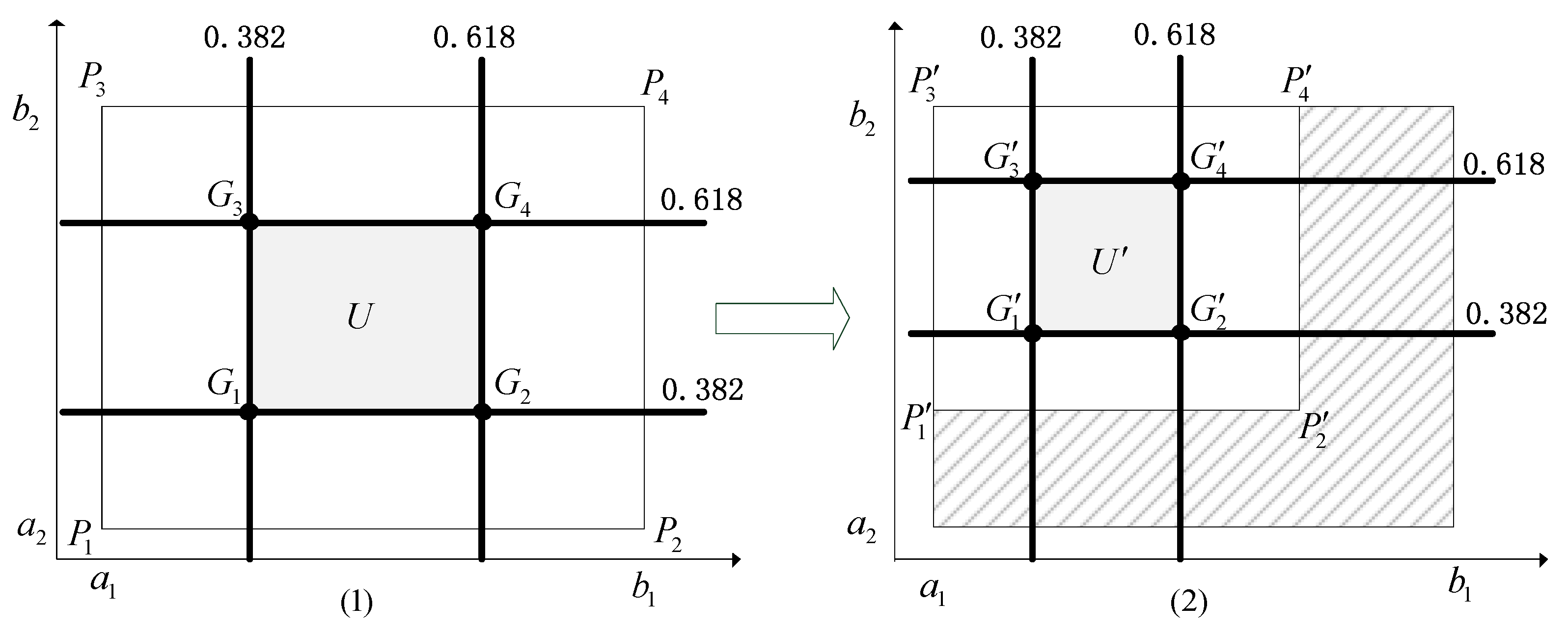
To solve for $\widehat{\mathsf{\theta }}$ in Equation (2), the CTOS & LSR method based on the optimum seeking method was proposed in this study. The optimum seeking method was first proposed by American mathematician Jack Keifer in the 1950s when studying the single-factor optimum seeking methods such as the golden section method (also called the 0.618 method). The purpose of the optimum seeking method was to reduce the number of experiments and to rapidly find out the optimal experimental points by using mathematical principles in the production and scientific research [37]. The CTOS method belongs to multivariate optimization approach, in which the effects of two variables or factors on the objective function are considered, and an optimal point is sought under a given constraint condition. The general idea of the CTOS method was as follows (see Figure 3): (I) The optimal point was first sought on a midline (e.g., red line); (II) Suppose the optimum was taken at point $P_1$, and a horizontal line passing through $P_1$ is drawn (green line); (III) Then the optimum was sought on this horizontal line (green line); (IV) Suppose the optimum occurs at point $P_2$, and an optimum was found on the vertical line (yellow line) passing through $P_2$; (V) The optimum was set at point $P_3$; (VI) The above procedures were repeated several times. The shadow indicated that this section was removed from the feasible region. Therefore, the feasible region was gradually narrowed until the final optimal point was found. For CTOS & LSR, the joint point parameters ${\mathsf{\alpha }}_1$ and ${\mathsf{\alpha }}_2$ were first estimated iteratively in the CTOS method, and then other parameters such as ${\mathsf{\beta }}_1$ to ${\mathsf{\beta }}_4$ in Equation (1) were estimated given ${\widehat{\mathsf{\alpha }}}_1$ and ${\widehat{\mathsf{\alpha }}}_2$ applying LSR. All estimates of these parameters in Equation (1) in each iteration were finally used to compute the values of the objective function (residual sum of squares).

The golden section method which is the foundation of many optimization algorithms was applied in this study to improve the computational efficiency of CTOS & LSR [37]. Two straight lines in each iteration were drawn at 0.382 and 0.618 of the value ranges of variable 1 and variable 2, respectively. The intersections of these straight lines were called interior points indicated by $G_1$, $G_2$, $G_3$, and $G_4$, which formed a rectangle $U$ (see Figure 4). The values of objective functions $f(G_1)$, $f(G_2)$, $f(G_3)$ and $f(G_4)$ were calculated. The interior point that had the minimum of the objective function was denoted as temp point. The rectangle $U\prime$ with the new interior points $G_1\prime$, $G_2\prime$, $G_3\prime$, and $G_4\prime$ was retained according to the temp point. After each iteration, the area of the rectangle $U\prime$ was gradually decreased, until the desired precision was obtained (Figure 4). A four-step iterative algorithm given below was applied to implement the CTOS & LSR.

Step 1:

The feasible region of variable 1 was ($a_1,b_1$) and the feasible region of variable 2 was ($a_2,b_2$). The four corners of a rectangle $U$ formed by the overlapped area were represented by $P_1$, $P_2$, $P_3$, and $P_4$, respectively. In rectangle $U$, four interior points $G_1$, $G_2$, $G_3$, and $G_4$ were obtained from the intersections of the following four lines:

$$x_1=a_1+0.382(b_1-a_1),$$

(3)

$$x_2=a_1+0.618(b_1-a_1),$$

(4)

$$y_1=a_2+0.382(b_2-a_2),$$

(5)

$$y_2=a_2+0.618(b_2-a_2),$$

(6)

The distance from the point $P_1$ with coordinates ($a_1,a_2$) to the point $P_4$ with coordinates ($b_1,b_2$) was calculated by the following formula:

$$D=\parallel p_1-p_4{\parallel }_2=\sqrt{{(a_1-a_2)}^2+{(b_1-b_2)}^2}.$$

(7)

Step 2:

θ in Equation (1) was estimated at each interior point with known coordinates by LSR, the objective functions $f(G_1)$, $f(G_2)$, $f(G_3)$ and $f(G_4)$ were computed, and the interior point that had the minimum objective function value was denoted as temp point.

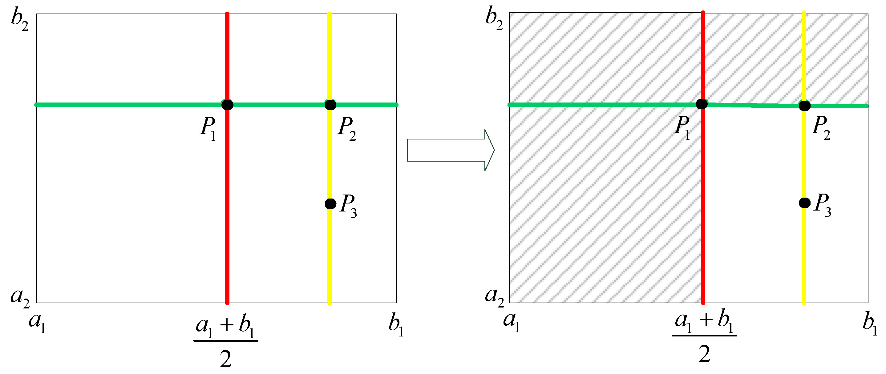
Step 3:

If $f(G_1)$ was the minimum, then the rectangle with $P_1{G}_4$ as the secondary diagonal was reserved; if $f(G_2)$ was the minimum, the rectangle with $G_3{P}_2$ as the secondary diagonal was reserved; if $f(G_3)$ was the minimum, the rectangle with $P_3{G}_2$ as the secondary diagonal was reserved; if $f(G_4)$ was the minimum, the rectangle with $G_1{P}_4$ as the secondary diagonal was reserved. The four corners of the new rectangle $U\prime$ were denoted as $P_1\prime$, $P_2\prime$, $P_3\prime$, and $P_4\prime$, respectively. $U\prime$, the four interior points$G_1\prime$, $G_2\prime$, $G_3\prime$, and $G_4\prime$ in the new rectangle also were determined by the golden section method. Computed distance would be $D^{\prime }=\parallel P_1\prime -P_4\prime {\parallel }_2$.

Step 4:

Steps 2 and 3 were repeated until a desired precision was obtained, for example, $\left|D^{\prime }\right|<0.00000001$. The final ${\widehat{\mathsf{\alpha }}}_1$ and ${\widehat{\mathsf{\alpha }}}_2$ were obtained, and then ${\widehat{\mathsf{\beta }}}_1-{\widehat{\mathsf{\beta }}}_4$ were estimated by LSR.

The CTOS & LSR with the four-step iterative algorithm for estimating in Equation (2) was implemented in VB version 6.0, see Appendix. It should be noted that, to simplify the LSR calculation, the model parameters ${\mathsf{\beta }}_1-{\mathsf{\beta }}_4$ in each iteration after giving ${\widehat{\mathsf{\alpha }}}_1$ and ${\widehat{\mathsf{\alpha }}}_2$ were estimated by transforming Equation (1) into the following linear form:

$$y={\mathsf{\beta }}_1{x}_1+{\mathsf{\beta }}_2{x}_2+{\mathsf{\beta }}_3{x}_3+{\mathsf{\beta }}_4{x}_4+\mathsf{\epsilon }$$

(8)

where, $x_1=h/H-1$, $x_2={(h/H)}^2-1$, $x_3={({\widehat{\mathsf{\alpha }}}_1-h/H)}^2{I}_1$, $x_4={({\widehat{\mathsf{\alpha }}}_2-h/H)}^2{I}_2$, $y={(d/D)}^2$, and the corresponding indicator variables $I_1$ and $I_1$ are given by

$$I_1=\frac{|({\widehat{\mathsf{\alpha }}}_1-h/H)|+({\widehat{\mathsf{\alpha }}}_1-h/H)}{2({\widehat{\mathsf{\alpha }}}_1-h/H)}$$

(9)

$$I_2=\frac{|({\widehat{\mathsf{\alpha }}}_2-h/H)|+({\widehat{\mathsf{\alpha }}}_2-h/H)}{2({\widehat{\mathsf{\alpha }}}_2-h/H)}$$

(10)

Therefore, Equation (8) was a typical linear model, which was easily solved by LSR.

2.4. ULSR Method

The method ULSR based on the minimization of the residual sum of squares has been commonly used to estimate parameters in forest growth and yield models. Equation (1) was difficult to solve directly using ULSR due to the unknown parameters ${\mathsf{\alpha }}_1$ and ${\mathsf{\alpha }}_2$ in both indicator variables $I_1$ and $I_2$. Based on Equations (9) and (10), we transformed Equation (1) to the following form:

$$y={\mathsf{\beta }}_1(x-1)+{\mathsf{\beta }}_2(x^2-1)+{\mathsf{\beta }}_3{({\mathsf{\alpha }}_1-x)}^2\frac{|({\mathsf{\alpha }}_1-x)|+({\mathsf{\alpha }}_1-x)}{2({\mathsf{\alpha }}_1-x)}+{\mathsf{\beta }}_4{({\mathsf{\alpha }}_2-x)}^2\frac{|({\mathsf{\alpha }}_2-x)|+({\mathsf{\alpha }}_2-x)}{2({\mathsf{\alpha }}_2-x)}+\mathsf{\epsilon }$$

(11)

This transformed Equation (11) is a general nonlinear model and could be directly estimated by ULSR.

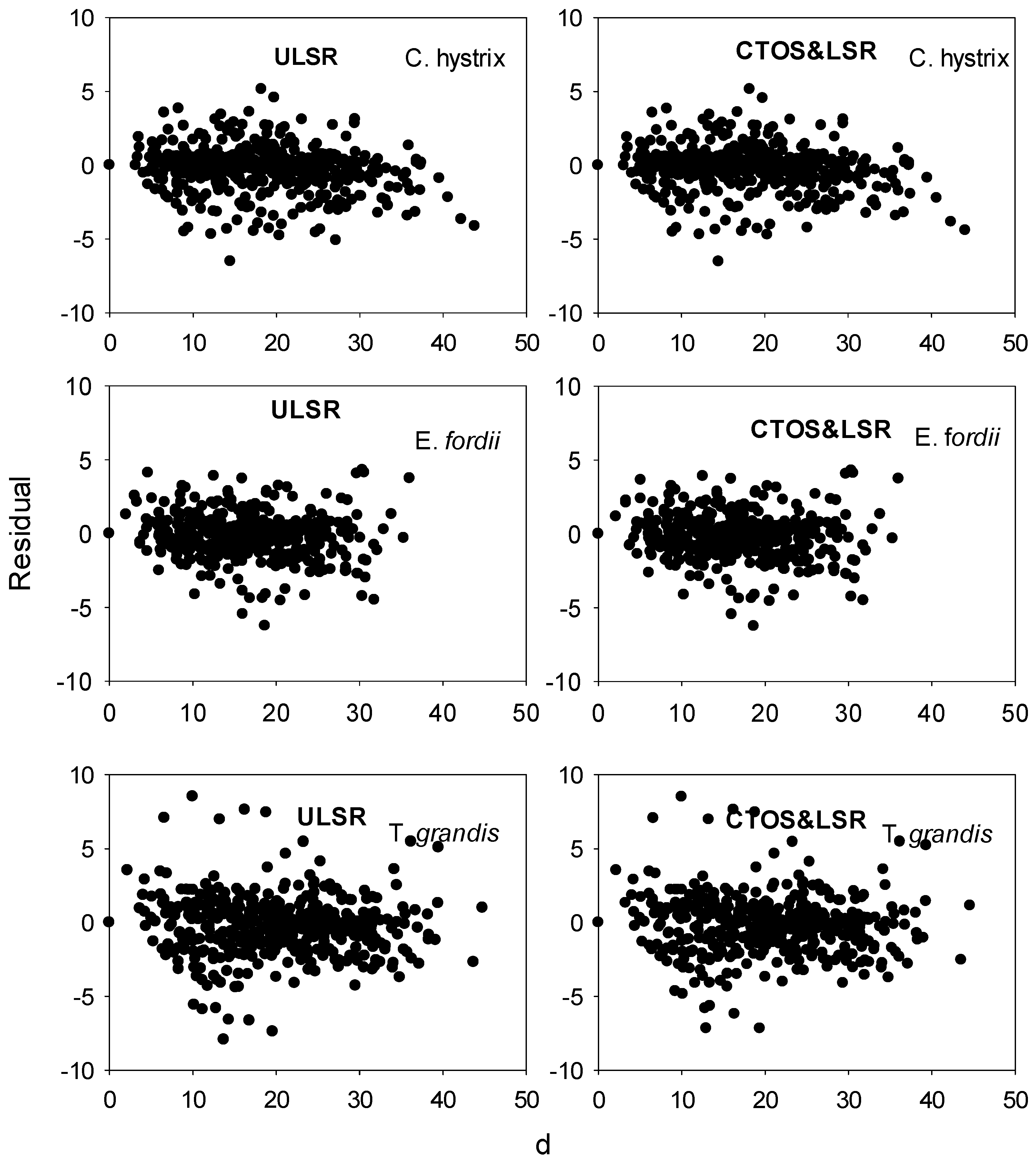
2.5. Taper Equation Evaluation

With application of Equation (1) the individual tree-level equation using sub-dataset from nine isolated dominant or codominant trees (Figure 2) and the population average-level equation using the full dataset of 120 trees (Table 1) were developed using both ULSR and CTOS & LSR. The predictive ability of Equation (1) at the individual tree-level obtained from the two methods was assessed using the coefficient of determination ($R^2$) and the residual sum of squares (RSS) statistics that are accounted for in Equations (12) and (13). The predictive ability of Equation (1) at the population average-level was assessed using $R^2$, RSS, the mean of prediction errors ($\overline{e}$) (Equation(14)), the variance of prediction errors (${\mathsf{\sigma }}^2$) (Equation (15)), and the root mean square error ($\mathsf{\delta }$) (Equation (16)) by a defined cross-validation [38,39].

$${\overline{R}}^2=1-\frac{{\displaystyle \sum {(y_i-{\widehat{y}}_i)}^2}}{{\displaystyle \sum {(y_i-\overline{y})}^2}}$$

(12)

$$\text{RSS}=\sum {(y_i-{\widehat{y}}_i)}^2$$

(13)

$$\overline{e}=\sum (y_i-{\widehat{y}}_i)/N$$

(14)

$${\mathsf{\sigma }}^2=\sum {(y_i-{\widehat{y}}_i)}^2/(N-1)$$

(15)

$$\mathsf{\delta }=\sqrt{{\overline{e}}^2+{\mathsf{\sigma }}^2}$$

(16)

where $y_i$ and ${\widehat{y}}_i$ are the observed and predicted dependent for the $i$th observation; $\overline{y}$ is the mean of the observed dependent, $N$ is the total number of observations; $\overline{e}$ and ${\mathsf{\sigma }}^2$ are the mean and variance of prediction errors, respectively; and $\mathsf{\delta }$ is the root mean square error that combines the mean bias and the variation of the residuals and was used as the primary criterion for taper equation evaluations [40].

In this study, the cross-validation meant that the full dataset was randomly divided into 10 sub-datasets, each having 12 trees and Equation (1) was fitted 10 times. Each time, one sub-dataset (i.e., a total of 12 trees) was removed from the full dataset and the remaining nine sub-datasets (i.e., a total of 108 trees) together were used to fit the equation using both methods of ULSR and CTOS & LSR. The equations obtained were then employed to make tree taper predictions for the removed sub-dataset and the differences between the estimated and observed values were calculated. After all the sub-datasets yielded the predicted values of tree taper, the statistics ($R^2$, $\text{RSS}$, $\overline{e}$, ${\mathsf{\sigma }}^2$ and $\mathsf{\delta }$) of the differences between the estimated and observed values were calculated. For details of the cross-validation approach, readers can refer to the studies by Vanclay [38] and Arlot and Celisse [39]. Moreover, all calculations were carried out using ForStat 2.2 version [41].

3. Results

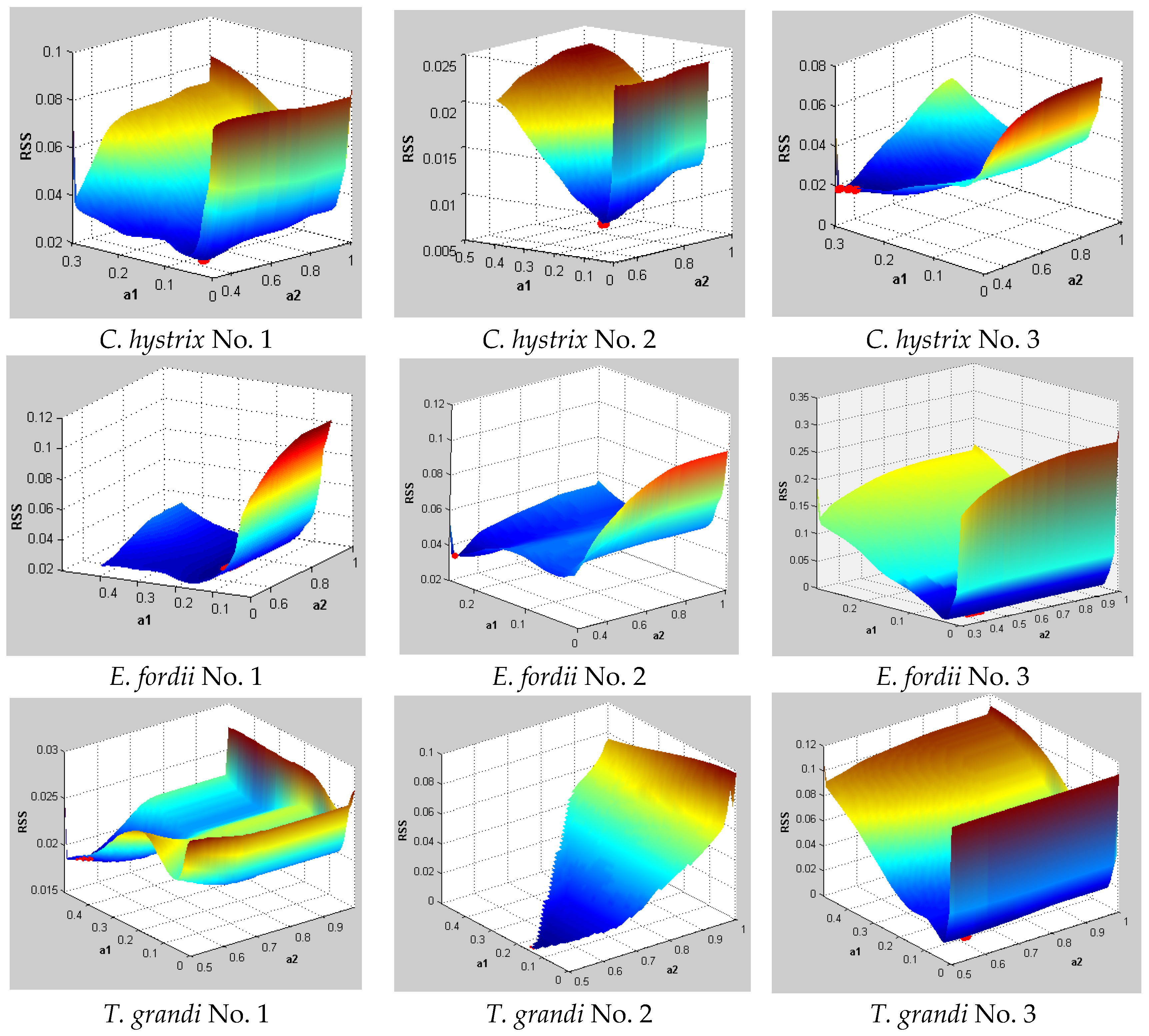
3.1. Taper Equation at Individual Tree-Level

Table 2. Parameter estimates and statistics of Equation (1) fitted by a combined method of constrained two-dimensional optimum seeking and least square regression (CTOS & LSR) and the unconstrained least square regression (ULSR) for nine individual trees (three trees from each species of C. hystrix, E. fordii, and T. grandis), ${\mathsf{\alpha }}_1-{\mathsf{\alpha }}_2$, joint point parameters; ${\mathsf{\beta }}_1-{\mathsf{\beta }}_4$, model parameters; $\text{RSS}$, residual sum of square; $R^2$, coefficient of determination.

Tree Species	No.	Method	${\mathsf{\alpha }}_{\mathbf{1}}$	${\mathsf{\alpha }}_{\mathbf{2}}$	${\mathsf{\beta }}_{\mathbf{1}}$	${\mathsf{\beta }}_{\mathbf{2}}$	${\mathsf{\beta }}_{\mathbf{3}}$	${\mathsf{\beta }}_{\mathbf{4}}$	$\mathbf{\text{RSS}}$	${\mathit{R}}^{\mathbf{2}}$
C. hystrix	(1)	CTOS & LSR	0.0579	0.3937	−2.8796	1.3293	139.5926	−3.368	0.0230	0.991
		ULSR	0.0585	0.3937	−2.8791	1.329	−3.3658	129.354	0.0230	0.991
	(2)	CTOS & LSR	0.0352	0.5093	−3.2136	1.6851	182.6908	−1.7546	0.0090	0.996
		ULSR	0.0356	0.5092	−3.213	1.6847	173.213	−1.7545	0.0090	0.996
	(3)	CTOS & LSR	0.2292	0.3783	−2.1126	0.8538	25.3279	−7.4583	0.0074	0.997
		ULSR	0.2812	0.3407	−2.1712	0.8912	32.6352	−22.27	0.0066	0.997
E. fordii	(1)	CTOS & LSR	0.1595	0.7361	−4.7264	2.3894	27.0427	−2.7965	0.0204	0.989
		ULSR	0.1649	0.7675	−5.9143	3.0609	21.8090	−3.4446	0.0206	0.989
	(2)	CTOS & LSR	0.2431	0.2818	−2.1716	0.9591	93.5096	−53.8856	0.0299	0.985
		ULSR	0.0603	0.8665	2.0566	−1.4212	92.6192	2.3332	0.0499	0.9774
	(3)	CTOS & LSR	0.0340	0.3631	−2.6455	1.3478	886.3202	−1.7084	0.0029	0.999
		ULSR	0.0342	0.3695	−2.6554	1.3541	844.7019	−1.667	0.0029	0.999
T. grandi	(1)	CTOS & LSR	0.3996	0.5837	−4.4012	2.3442	7.9341	−5.2571	0.0179	0.990
		ULSR	0.4916	0.5549	−4.0975	2.1651	9.0758	−9.5458	0.0190	0.990
	(2)	CTOS & LSR	0.1385	0.6910	−2.8939	1.4189	33.1479	−1.2589	0.0026	0.999
		ULSR	0.1403	0.8530	−8.4821	4.5000	27.9491	−4.2567	0.0026	0.999
	(3)	CTOS & LSR	0.0325	0.5609	−3.4995	1.7276	558.3056	−2.2966	0.0134	0.995
		ULSR	0.0328	0.5611	−3.5011	1.7286	532.4962	−2.2968	0.0134	0.995

shows the fitting results including parameter estimates and statistics for nine individual trees using both ULSR and CTOS & LSR. The fitting of Equation (1) using both ULSR and CTOS & LSR for each tree reached convergence with meaningful parameter estimates. The fitting of Equation (1) using the ULSR did not reach convergence with one-time starting values. Thus, different starting values were needed to make the equation convergence with the global minimum. However, with CTOS & LSR, Equation (1) easily converged for all nine individual trees. The differences of some parameter estimates of Equation (1) between ULSR and CTOS & LSR for all trees were significant at a risk level of α = 0.05. For example, for E. fordii, the estimate of the joint point parameter ${\mathsf{\alpha }}_1=0.2431$ from ULSR was almost four times larger than that (${\mathsf{\alpha }}_1=0.0603$) from CTOS & LSR, and the estimate of joint point parameter ${\mathsf{\alpha }}_2=0.2818$ from ULSR was almost one third of the corresponding parameter estimate (${\mathsf{\alpha }}_1=0.8665$) from CTOS & LSR.

A t-test showed that the mean biases of all trees (Table 2) for the two methods were not significantly different from zero (p > 0.05). The coefficients of determination $R^2$ of each tree for the two methods were very high. For many trees, such as C. hystrix No. 1 and No. 2, E. fordii No. 3, T. grandis No. 2 and No. 3, the two methods had identical fitting precisions. However, for several trees, such as E. fordii No. 2 and T. grandis No. 1, the RSS and $R^2$ from the CTOS & LSR method were slightly better than those of the corresponding trees obtained from ULSR. Especially for E. fordii No. 2, the value of $\text{RSS}$ from CTOS & LSR was 40% smaller than that from ULSR. These results suggested that the fitting accuracy of Equation (1) at the individual tree-level obtained from CTOS & LSR was slightly higher than that of the corresponding equation obtained from ULSR for those trees whose taper curve has more variation.

For testing CTOS & LSR, the residuals of Equation (1) with the whole feasible ranges ($0<a_1<a_2<1$) of the two joint point parameters ${\mathsf{\alpha }}_1$ and ${\mathsf{\alpha }}_2$ by step size 0.01 and satisfying the constrained conditions ${\mathsf{\alpha }}_1<{\mathsf{\alpha }}_2$ were calculated for the nine individual trees. The residual distribution of each tree is displayed in Figure 5. The red points in Figure 5 denote the corresponding final solutions of Equation (1) obtained by CTOS & LSR for each individual tree. The points with the minimum $RSS$ of Equation (1) with the constrained $0<a_1<a_2<1$ were almost identical to the corresponding red points that were determined by CTOS & LSR for the nine individual trees. This indicated that the CTOS & LSR proposed in this study could minimize the RSS of Equation (1) more efficiently.

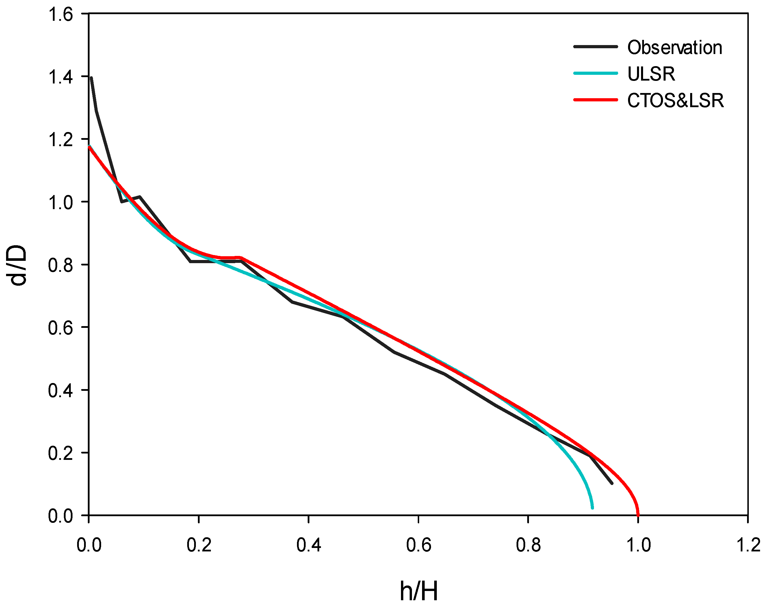
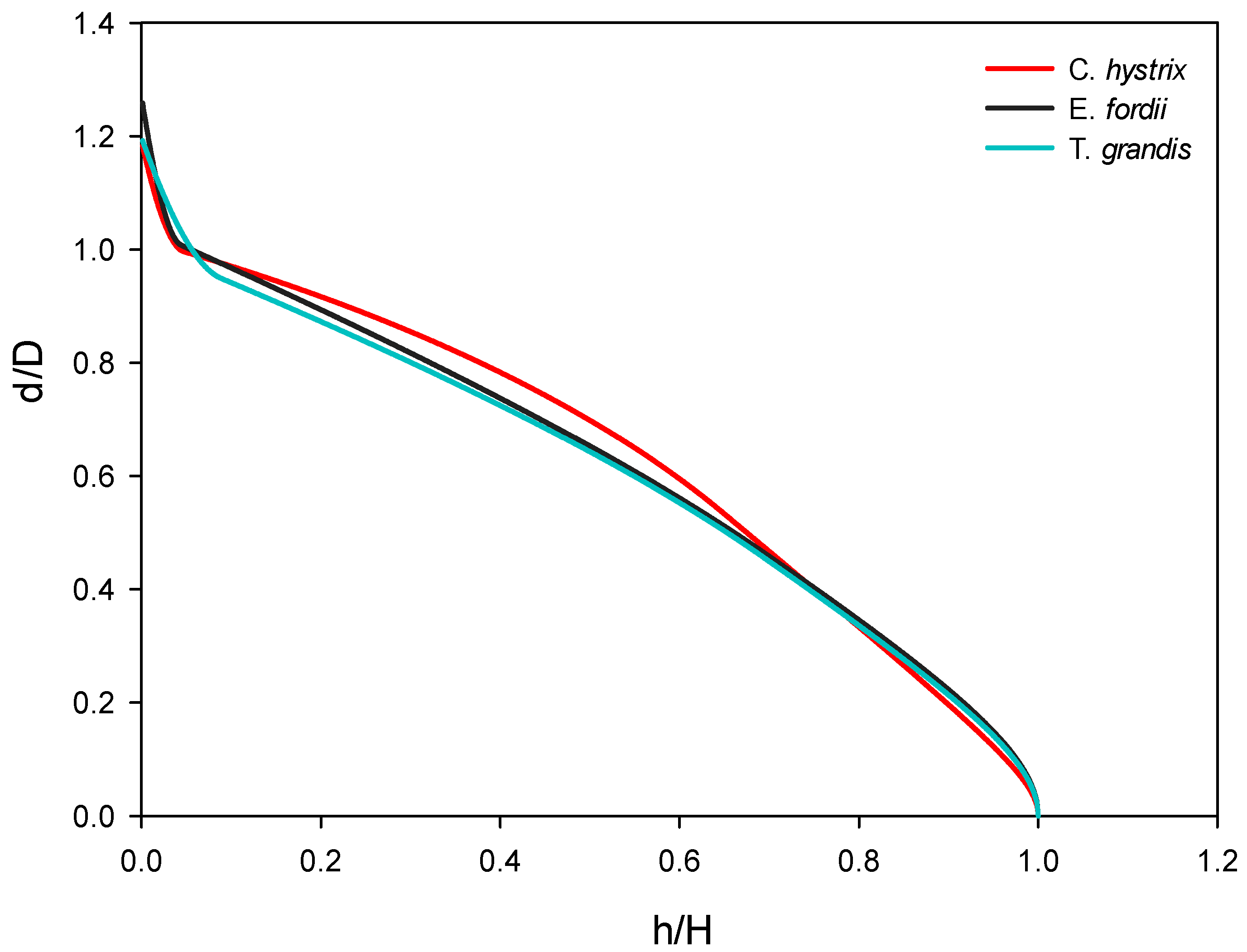
3.2. Taper Equation at Population Average-Level

The parameter estimates of Equation (1) obtained from both ULSR and CTOS & LSR based on the full dataset (Table 1) were listed in

Table 3. Parameter estimates of Equation (1) obtained from both ULSR and CTOS & LSR based on the full data-set from three species (C. hystrix, E. fordii, and T. grandi), ${\mathsf{\alpha }}_1-{\mathsf{\alpha }}_2$, joint point parameters; ${\mathsf{\beta }}_1-{\mathsf{\beta }}_4$, model parameters.

Tree Species	Method	${\mathsf{\alpha }}_{\mathbf{1}}$	${\mathsf{\alpha }}_{\mathbf{2}}$	${\mathsf{\beta }}_{\mathbf{1}}$	${\mathsf{\beta }}_{\mathbf{2}}$	${\mathsf{\beta }}_{\mathbf{3}}$	${\mathsf{\beta }}_{\mathbf{4}}$
C. hystrix	ULSR	0.0481	0.6479	−3.6251	1.7049	158.3459	−2.1074
	CTOS & LSR	0.0474	0.6479	−3.624	1.7043	169.9877	−2.1063
E. fordii	ULSR	0.0444	0.7190	−2.5992	1.1148	257.2861	−0.7817
	CTOS & LSR	0.0440	0.6910	−2.4256	1.0154	274.0969	−0.6923
T. grandis	ULSR	0.0903	0.6993	−2.5923	1.1282	51.1553	−0.9210
	CTOS & LSR	0.0890	0.6910	−2.5193	1.0861	52.6617	−0.8752

. Equation (1) for each tree species reached convergence with meaningful parameter estimates using either method. As with Equation (1) at the individual tree-level, different starting values were required for ULSR to make Equation (1) converge. The parameter estimates of Equation (1) with ULSR and CTOS & LSR for each species were not identical. Especially for C. hystrix, the value of ${\mathsf{\beta }}_3$ estimated by ULSR was 7% larger than that estimated by CTOS & LSR.

Based on cross-validation, the assessment results of five prediction statistics [Equations (12) and (16)] of Equation (1) using both ULSR and CTOS & LSR for the three tree species are listed in

Table 4. The statistics of Equation (1) fitted by the combination method of constrained two-dimensional optimum seeking and least square regression (CTOS & LSR) and the unconstrained least square regression (ULSR) for three trees species (C. hystrix, E. fordii, and T. grandis) based on cross-validation approach.

Tree Species	Method	$\mathbf{\text{RSS}}$	${\mathit{R}}^{\mathbf{2}}$	$\overline{\mathit{e}}$	${\mathsf{\sigma }}^{\mathbf{2}}$	$\mathsf{\delta }$
C. hystrix	ULSR	3.404	0.959	−0.2518	2.2898	1.5340
	CTOS & LSR	3.404	0.959	−0.1814	2.0989	1.4601
E. fordii	ULSR	4.401	0.953	−0.1568	2.1878	1.4874
	CTOS & LSR	4.401	0.953	−0.1611	2.1753	1.4837
T. grandis	ULSR	3.479	0.962	−0.2211	3.7328	1.9446
	CTOS & LSR	3.479	0.962	−0.1870	3.5452	1.8921

$\text{RSS}$, residual sum of square; $R^2$, coefficient of determination; $\overline{e}$, mean of prediction errors; ${\mathsf{\sigma }}^2$, variance of prediction errors; $\mathsf{\delta }$, root mean square error.

. The mean prediction errors $\overline{e}$ of Equation (1) for each tree species using either method were very small. Equation (1) for each tree species using both ULSR and CTOS & LSR slightly over-predicted the $d^2/D^2$. The coefficient of determination $R^2$ and $\text{RSS}$ of Equation (1) for each tree species from ULSR and CTOS & LSR were correspondingly identical. The prediction accuracies of Equation (1) for each tree species from CTOS & LSR were much higher than those of Equation (1) when the $d^2/D^2$ was estimated using from ULSR. For example, the values of ${\mathsf{\sigma }}^2$ and $\mathsf{\delta }$ of Equation (1) from CTOS & LSR for each tree species were smaller than those of Equation (1) from ULSR. Especially for C. hystrix, the variance of prediction errors ${\mathsf{\sigma }}^2$ from CTOS & LSR was 8.34% smaller than those from ULSR, and the value of root mean square error $\mathsf{\delta }$ from CTOS & LSR was 5% smaller than those from ULSR. This suggested that the prediction ability of Equation (1) using CTOS & LSR was more powerful than that of Equation (1) using ULSR.

The residuals of Equation (1) for each tree species using both ULSR and CTOS & LSR were plotted against the observed values (Figure 6). The results showed that Equation (1) for each tree species using either ULSR or CTOS & LSR did not lead to any trend of heteroscedasticity, which further indicated that Equation (1) was a better segmented taper equation for the prediction of tree taper.

4. Discussion

Equation (1) is able to describe the shape of a tree. The bottom trunk section, which includes the butt, is modeled as a frustum of a neiloidal solid, the middle of the trunk is assumed to take the shape of a frustum of a parabolodial solid, and the top portion is assumed to be conoid [13]. In this system, three additive equations were grafted together by incorporating two joint points between the three segments. The joint point parameters ${\mathsf{\alpha }}_1$ and ${\mathsf{\alpha }}_2$ with the constrained condition $0<{\mathsf{\alpha }}_1<{\mathsf{\alpha }}_2<1$ in Equation (1) were previously commonly estimated by ULSR and SE, which made the results of the equation uncertain. We proposed the CTOS & LSR method to estimate the parameters of Equation (1). It was based on the constrained two-dimensional optimum seeking algorithm with Hua Luogeng’s theory [36]. The CTOS & LSR method was evaluated using the stem analysis data sets of three tropical precious tree species C. hystrix, E. fordii, and T. grandis in the southwest of China. Our results (Table 2 and Table 4) show that this method is more reliable than ULSR for estimating the parameters in the segmented taper equation.

The literature show that ULSR is a widely used method for parameter estimation [15,24,28,29,30,31,32]. This method was also applied in the CTOS & LSR. For each iterative calculation in CTOS & LSR, the CTOS was first used to estimate parameters ${\mathsf{\alpha }}_1$ and ${\mathsf{\alpha }}_2$, after the two joint point parameters were determined, other remaining parameters in Equation (1) were estimated by LSR without constraint. The parameter estimates of Equation (1) for the two methods were obtained by minimizing the similar objective function (residual sum of squares). However, for ULSR, the estimates of parameters may fall out of the feasible range and make the results meaningless. For example, for the individual tree of E. fordii (Figure 7), the fitting accuracies of Equation (1) obtained from ULSR ($RSS=0.0460$, $R^2=0.9791$), and CTOS & LSR ($RSS=0.0391$, $R^2=0.982$) were almost similar and very high (Figure 7). However, the estimate of ${\mathsf{\alpha }}_2$ from ULSR is ${\widehat{\mathsf{\alpha }}}_2=1.3130$ (the other estimate was ${\widehat{\mathsf{\alpha }}}_1=0.1915$), which was larger than one and out of the feasible range. For CTOS & LSR, the estimates of ${\mathsf{\alpha }}_1$ and ${\mathsf{\alpha }}_2$ were 0.2692 and 0.6943; they were within the feasible range. Figure 7 also shows that the predicted taper curve from ULSR almost tends to zero when the relative height $h/H$ is just 0.92, which conflicts with the assumption that the relative outside bark diameter $d/D$ should be equal to zero at the relative height $h/H=1$. This situation always occurred in our preliminary analyses.

The overall prediction accuracies of Equation (1) at individual tree-levels and population average-levels from CTOS & LSR were much larger than those from ULSR (Table 2 and Table 4). This is due to the fact that the optimum solutions of Equation (1) obtained from CTOS & LSR were closer to actual values than these obtained from ULSR (Figure 5). In addition, the ULSR approach does not always converge for parameter estimation and this problem becomes more serious while fitting the taper equation at the individual tree-level. This is because the convergence of ULSR based on the iteration optimization algorithm, i.e., Gauss-Newton, depends largely on the given initial values of the parameters. In contrast, CTOS & LSR does not have a divergence problem. We also tried using other existing constrained optimization method e.g., simplex method and constrained Newton Raphson method, to estimate the parameters in Equation (1), but these methods failed to converge for some individual trees or tree species. Especially for the simplex method, the computational speed was also very slow. Besides forestry, CTOS & LSR could be also applied in agricultural engineering, industry or other fields requiring optimal selection of parameters. It is to be noted that the CTOS & LSR method only works on unimodal models. For multi-modal functions, there is no guarantee that the solutions of CTOS & LSR are the global optimum. We will focus on this limitation of the method in our future work.

Equation (1) with the estimates of parameters obtained from CTOS & LSR (Table 3) could be used to demonstrate differences of tree taper among three species C. hystrix, E. fordii, and T. grandis. The prediction accuracy with Equation (1) at the population average-level for each tree species is high (Figure 8). In addition, there are apparent differences among the tree taper of the three tropical precious tree species. For example, when the range of $h/H$ was from 0.00 to 0.03, the values of $d/D$ for T. grandis were much larger than those for the other two species (C. hystrix and E. fordii), which have almost the same $d/D$. When the range of $h/H$ was from 0.03 to 0.7, the values of $d/D$ for C. hystrix was the largest, following by E. fordii and T. grandis. When $h/H$ is larger than 0.8, the three species have the same tree taper. Equation (1) also could be used to describe differences in tree taper between individual trees.

Measuring tree diameter and height may be subject to errors, even though stand and tree variables are commonly assumed to be measured without error [42,43]. The measurement errors made by field crew or faulty instrument or both might be substantial [42]. In all existing taper equations including Equation (1), it is assumed that (i) the dependent variable is a random variable; and (ii) the independent variables are fixed and measured without errors. It is well known that the violation of the second assumption may lead to biased estimation of parameters and (or) of the standard errors of the parameters, and consequently to misleading the hypothesis test [44,45]. If the predictor variables in Equation (1) are considered to have measurement errors, a new parameter estimation approach needs to be developed. We are in the process of developing such a method to deal with this problem.

5. Conclusions

In this study, the CTOS & LSR was proposed as an improved method to estimate the parameters in the Equation (1). This method was compared with ULSR for both individual tree-level equation and the population average-level equation using data from three tree species including C. hystrix, E. fordii, and T. grandis in the southwest of China. The differences between CTOS & LSR and ULSR were found to be significant. The segmented taper equation estimated using CTOS & LSR resulted in not only increased prediction accuracy, but also guaranteed the parameter estimates in a more meaningful way. It is thus recommended that the CTOS & LSR should be a preferred choice for this application.

References

1. Demaerschalk, J.P. Converting volume equations to compatible taper equations. For. Sci. 1972, 18, 241–245. [Google Scholar]
2. Duan, A.; Zhang, S.; Zhang, X.; Zhang, J. Development of a stem taper equation and modelling the effect of stand density on taper for Chinese fir plantations in Southern China. PeerJ 2016, 4, e1929. [Google Scholar] [CrossRef] [PubMed]
3. Kozak, A. A variable-exponent taper equation. Can. J. For. Res. 1988, 18, 1363–1368. [Google Scholar] [CrossRef]
4. Fang, Z.; Borders, B.E.; Bailey, R.L. Compatible volume taper models for loblolly and slash pine based on system with segmented-stem form factors. For. Sci. 2000, 46, 1–12. [Google Scholar]
5. Jordan, L.; Berenhaut, K.; Souter, R.; Daniels, R.F. Parsimonious and completely compatible taper, total and merchantable volume models. For. Sci. 2005, 51, 578–584. [Google Scholar]
6. Kozak, A.; Munro, D.O.; Smith, J.H.G. Taper functions and their application in forest inventory. For. Chron. 1969, 45, 278–283. [Google Scholar] [CrossRef]
7. Ormerod, D.W. A simple bole model. For. Chron. 1973, 49, 136–138. [Google Scholar] [CrossRef]
8. Amidon, E.L. A general taper functional form to predict bole volume for five mixed-conifer species in Califomia. For. Sci. 1984, 30, 166–171. [Google Scholar]
9. Biging, G.S. Taper equations for second-growth mixed conifers in northern California. For. Sci. 1984, 30, 1103–1117. [Google Scholar]
10. Thomas, C.E.; Parresol, B. Simple, flexible, trigonometric taper equations. Can. J. For. Res. 1991, 21, 1132–1137. [Google Scholar] [CrossRef]
11. Sharma, M.; Oderwald, R.G. Dimensionally compatible volume and taper equations. Can. J. For. Res. 2001, 31, 797–803. [Google Scholar] [CrossRef]
12. Zakrzewski, W.T.; MacFarlane, D.W. Regional stem profile model for cross-border comparisons of harvested red pine (Pinus resinosa Ait.) in Ontario and Michigan. For. Sci. 2006, 52, 468–475. [Google Scholar]
13. Max, T.A.; Burkhart, H.E. Segmented polynomial regression applied to taper equations. For. Sci. 1976, 22, 283–289. [Google Scholar]
14. Cao, Q.V.; Burkhart, H.E.; Max, T.A. Evaluations of two methods for cubic volume prediction of loblolly pine to any merchantable limit. For. Sci. 1980, 26, 71–80. [Google Scholar]
15. Valenti, M.; Cao, Q. Use of crown ratio to improve loblolly pine taper equations. Can. J. For. Res. 1986, 16, 1141–1145. [Google Scholar] [CrossRef]
16. Parresol, B.; Hotvedt, J.; Cao, Q. A volume and taper prediction system for bald cypress. Can. J. For. Res. 1987, 17, 250–259. [Google Scholar] [CrossRef]
17. Jiang, L.; Liu, R. Segmented taper equations with crown ratio and stand density for Dahurian Larch (Larix gmelinii) in Northeastern China. J. For. Res. 2011, 22, 347–352. [Google Scholar] [CrossRef]
18. Newnham, R.M. Variable-form taper equation for four Alberta tree species. Can. J. For. Res. 1992, 22, 210–223. [Google Scholar] [CrossRef]
19. Muhairwe, C.K. Tree form and taper variation over time for interior lodgepole pine. Can. J. For. Res. 1994, 24, 1904–1913. [Google Scholar] [CrossRef]
20. Valentine, H.T.; Gregoire, T.G. A switching model of bole taper. Can. J. For. Res. 2001, 31, 1400–1409. [Google Scholar] [CrossRef]
21. Lee, W.K.; Seo, J.H.; Son, Y.M.; Lee, K.H.; von Gadow, K. Modeling stem profiles for Pinus densiflora in Korea. For. Ecol. Manag. 2003, 172, 69–77. [Google Scholar] [CrossRef]
22. Zeng, W.; Liao, Z. Research of taper equation. Sci. Silvae Sin. 1997, 33, 127–132, (In Chinese with English Summary). [Google Scholar]
23. Demaerschalk, J.P.; Kozak, A. The whole-bole system: A conditioned dual equation system for precise prediction of tree profiles. Can. J. For. Res. 1997, 7, 488–497. [Google Scholar] [CrossRef]
24. Cao, Q.V.; Wang, J. Calibrating fixed- and mixed-effects taper equations. For. Ecol. Manag. 2011, 262, 671–673. [Google Scholar] [CrossRef]
25. Sabatia, C.O.; Burkhart, H.E. On the use of upper stem diameters to localize a segmented taper equation to new trees. For. Sci. 2015, 61, 411–423. [Google Scholar] [CrossRef]
26. Rojo, A.; Perales, X.; Sanchez-Rodriguez, F.; Alvarez-Gonzalez, J.G.; von Gadow, K. Stem tape functions for maritime pine (Pinus pinaster Ait.) in Galicia (Northwestern Spain). Eur. J. For. Res. 2005, 124, 177–186. [Google Scholar] [CrossRef]
27. Jiang, L.; Brooks, J.R.; Wang, J. Compatible taper and volume equations for yellow-poplar in West Virginia. For. Ecol. Manag. 2005, 213, 399–409. [Google Scholar] [CrossRef]
28. Figueiredo-Filho, A.; Borders, B.E.; Hitch, K.L. Taper equations for Pinus taeda plantations in Southern Brazil. For. Ecol. Manag. 1996, 83, 39–46. [Google Scholar] [CrossRef]
29. Muhairwe, C.K. Taper equations for Eucalyptus pilularis and Eucalyptus grandis for the north coast in New South Wales, Australia. For. Ecol. Manag. 1999, 113, 251–269. [Google Scholar] [CrossRef]
30. Sharma, M.; Burkhart, H.E. Selecting a level of conditioning for the segmented polynomial taper equation. For. Sci. 2003, 49, 324–330. [Google Scholar]
31. Coble, D.W.; Hilpp, K. Compatible cubic-foot stem volume and upper-stem diameter equations for semi-intensive plantation grown loblolly pine trees in East Texas. South J. Appl. For. 2006, 30, 132–141. [Google Scholar]
32. Trincardo, G.; Burkhart, H.E. A generalized approach for modeling and localizing stem profile curves. For. Sci. 2006, 52, 670–682. [Google Scholar]
33. Brooks, J.R.; Jiang, L.; Ozcelik, R. Compatible stem volume and taper equations for Brutian Pine, Taurus Cedar, and Taurus Fir in Turkey. For. Ecol. Manag. 2008, 256, 147–151. [Google Scholar] [CrossRef]
34. Pang, L. Stand Harvest Analysis and Information Management System for Target Tree. Ph.D. Thesis, Chinese Academy of Forestry, Beijing, China, 2015. [Google Scholar]
35. Tang, S.; Li, Y.; Wang, Y. Simultaneous equations, errors-in-variable models, and model integration in systems ecology. Ecol. Model. 2001, 142, 285–294. [Google Scholar] [CrossRef]
36. Hua, L. Optimum Seeking Methods; Science Press: Beijing, China, 1967. [Google Scholar]
37. Schwefel, P.H.P. Evolution and Optimum Seeking: The Sixth Generation; John Wiley & Sons, Inc.: New York, NY, USA, 1993. [Google Scholar]
38. Vanclay, J.K. Modelling Forest Growth and Yield: Applications to Mixed Tropical Forests; CAB International: Wallingford, UK, 1994. [Google Scholar]
39. Arlot, S.; Celisse, A. A survey of cross-validation procedures for model selection. Statist. Surv. 2010, 4, 40–79. [Google Scholar] [CrossRef]
40. Yang, Y.; Huang, S. Comparison of different methods for fitting nonlinear mixed forest models and for making predictions. Can. J. For. Res. 2011, 41, 1671–1686. [Google Scholar] [CrossRef]
41. Tang, S.Z.; Lang, K.J.; Li, H.K. Statistics and Computation of Biomathematical Models (ForStat Course); Science Press: Beijing, China, 2008. (In Chinese) [Google Scholar]
42. Omule, A.Y. Personal bias in forest measurement. For. Chron. 1980, 56, 222–224. [Google Scholar] [CrossRef]
43. Gertner, G.Z. The sensitivity of measurement error in stand volume estimation. Can. J. For. Res. 1990, 20, 800–804. [Google Scholar] [CrossRef]
44. Fuller, W.A. Measurement Error Models; John Wiley and Sons: New York, NY, USA, 1987. [Google Scholar]
45. Rencher, A.C.; Schaalje, G.B. Linear Models in Statistics, 2nd ed.; John Wiley and Sons: New York, NY, USA, 2008. [Google Scholar]
Figure 1. Location of study area: Experimental Center of Tropical Forestry, Chinese Academy of Forestry Sciences and spatial distribution of 30 sample plots.
Forests 07 00194 g001
Figure 2. Observed height (h) above the ground-outside bark diameter (d) curves for nine dominant or codominant trees.
Forests 07 00194 g002
Figure 3. The general idea of the constrained two-dimensional optimum seeking method, a1 and b1 are the lower and upper limits for the feasible region of the first parameter, respectively; a2 and b2 are the lower and upper limits for the feasible region of the second parameter, respectively, P1, P2, and P3 are corresponding optimal points for different iterative steps.
Forests 07 00194 g003
Figure 4. Diagram of the combination of constrained two-dimensional optimum seeking method and least square regression (CTOS & LSR), P 1 , P 2 , P 3 , and P 4 are four corners of the rectangle U determined by the feasible region of the estimated two-dimensional variables, G 1 , G 2 , G 3 , and G 4 are interior points of U determined by the golden section method, P 1 , P 2 , P 3 , and P 4 are four corners of the rectangle U obtained by one iteration calculation of CTOS & LSR; G 1 , G 2 , G 3 , and G 4 are interior points of U determined by the golden section method.
Forests 07 00194 g004
Figure 5. The residual distribution of Equation (1) with the whole feasible range ( 0 < α 1 < α 2 < 1 ) of joint points α 1 and α 2 by step size 0.01 and satisfying the constrained conditions α 1 < α 2 calculated by the combination of the constrained two-dimensional optimum seeking method and the least square regression (CTOS & LSR) for the nine individual trees. The red points denote the corresponding final solutions of Equation (1) obtained by CTOS & LSR for each individual tree.
Forests 07 00194 g005
Figure 6. Residuals of the Equation (1) for the three tree species C. hystrix, E. fordii. and T. grandi using both the combination method of constrained two-dimensional optimum seeking and least square regression (CTOS & LSR) and the unconstrained least square regression (ULSR) plotted against the observed values based on cross-validation.
Forests 07 00194 g006
Figure 7. Observed relative outside bark diameters at different relative height location (black line) for an individual tree of E. fordii. The predicted taper curves from the Equation (1) using both the combination method of constrained two-dimensional optimum seeking and least square regression (CTOS & LSR) (red line) and the unconstrained least square regression (ULSR) (blue line) are shown.
Forests 07 00194 g007
Figure 8. The predicted taper curves from Equation (1) using the combined method of constrained two-dimensional optimum seeking and least square regression (CTOS & LSR) for the three tree species C. hystrix (red line), E. fordii (black line), and T. grandi (blue line) at the population average level.
Forests 07 00194 g008