1. Introduction
While soil moisture is quantitatively negligible in the global water budget [
1], seldom would anyone doubt its importance in studies concerning hydrological and other land surface processes. Soil water is not only a necessity for growth of vegetation and other soil-born living beings, but also one of the major controlling factors in partitioning of surface runoff and infiltration, as well as in partitioning of latent and sensible heat at ground surface [
2]. In addition, at large scales, the influence of soil moisture is strong enough to change regional weather patterns, e.g., precipitation [
3]. Specifically in hydrological studies, grid mean or representative soil moisture content is normally required, for example, to initiate and validate forecasting models [
4,
5] and to estimate regional water storage [
6]. However, soil moisture obtained through ground-based measuring campaigns is basically limited to point scales, resulting in scale mismatch between observations and applications of soil moisture. This problem and the work of upscaling have challenged researchers for a long time, mainly because of the strong spatial variation of soil moisture [
7]. After decades of development, techniques of remote sensing are now able to estimate regional moisture content in shallow soils [
8,
9]. Nonetheless, sub-pixel distribution and variation of soil moisture obtained through ground-based monitoring are still indispensable in validating and correcting these estimations [
10], as well as in data assimilation [
11].
Numerous studies on spatial variability of soil moisture across the planet have been presented in recent decades, and the relationship between spatial variance and spatial mean is one of the major frameworks in investigating spatio-temporal variability of soil moisture patterns [
12]. Many studies of various areas have found significant correlations between the two statistical variables, but forms of the correlations are still highly controversial. From reports, spatial variance of soil moisture could be positively [
13,
14,
15] or negatively [
16,
17,
18] correlated with spatial mean, and it frequently showed an upward convex correlation [
19,
20,
21,
22] with spatial mean. Comparisons inferred that these correlations may vary among locations with, for example, different climate [
23,
24,
25], soil texture [
26,
27], and vegetation cover [
25,
28], as well as the spatial scale of the studied area [
29,
30].
Uncertainty regarding the spatial variance-mean relationship indicates that mean soil moisture is accompanied by some other factors in determining spatial variance [
25,
31,
32]. For this reason, many authors have tried to quantify contributions of various factors on spatial variance. For example, Western et al. (1998) [
15], among others [
32], concluded that the contribution of terrain indices varied from 22% in the dry season to 61% in the wet season. Instead of geo-surveying, Albertson and Montaldo (2003) [
19] developed a conservative equation for spatial variance, and studied the covariance between soil moisture and sorts of water fluxes (i.e., infiltration, drainage, evapotranspiration, and horizontal redistribution) by a simulation approach. Teuling and Troch (2005) [
33] extended this work and further categorized influence factors into three types--vegetation, soil, and topography--by merging together in the equation contribution components of each type. Based on stochastic methods, Vereecken et al. (2007) [
22] studied the sensitivity of soil moisture variance to parameters of soil hydraulic properties, and suggested that heterogeneity of soil texture could be inversely estimated from spatially distributed measurements of soil moisture content. However, application of these measures are highly dependent on spatially dense monitoring of soil moisture as well as the factors of interest, data on which are normally hard to obtain. Moreover, contributors that are of interest and not of interest may be interdependent and thus increase the challenge to separate the contribution of one factor from another. More recently, Mittelbach and Seneviratne (2012) [
12] suggested that soil moisture could be divided into two parts, i.e., the temporal mean and temporal anomaly, and spatial variance could consequently be decomposed into spatial variance of temporal mean, that of temporal anomalies, and a covariance of temporal mean and temporal anomalies. This method was then applied to evaluate spatial variances of soil moisture across Switzerland, with the conclusion that temporal dynamic factors contributed only 9% on average. A similar result was obtained by Brocca et al. (2014) [
34] in their study of the global variance of soil moisture. More recently, Gao et al. (2015) [
35] also studied the contributions of both temporal dynamic and time-invariant factors on different scales in west China; they found, however, the time invariant contributor gradually lost its dominance as the scale got larger.
Although spatial variability of soil moisture varies among different locations, it often shows some features of temporal stability in a specific area. From this perspective, Vachaud et al. (1985) [
36] proposed the concept of rank stability, referring to the time stability of the rank of individual observations in the probability distribution function of the whole population [
29]. Studies have showed that although rank of sites may not be absolutely consistent all through the monitoring, it may show some similarities at different time points. This method is recognized as a help approach in improving monitoring strategies and upscaling of soil moisture [
37,
38].
In this study, spatial variability of soil moisture within a 7 km
2 forest catchment in semi-humid north China was examined, basically from three aspects: (i) examination of the relationship between spatial mean and spatial variance; (ii) quantification of the contributions of temporal dynamic and time-invariant factors to the spatial variance of soil moisture, by applying Mittelbach and Seneviratne’s (2012) method [
12]; and (iii) determination of the site ranks based on absolute deviation from spatial mean of each monitoring site, and then the examination of temporal stability of the spatial variability by comparing site ranks in different periods.
3. Study Area and Dataset
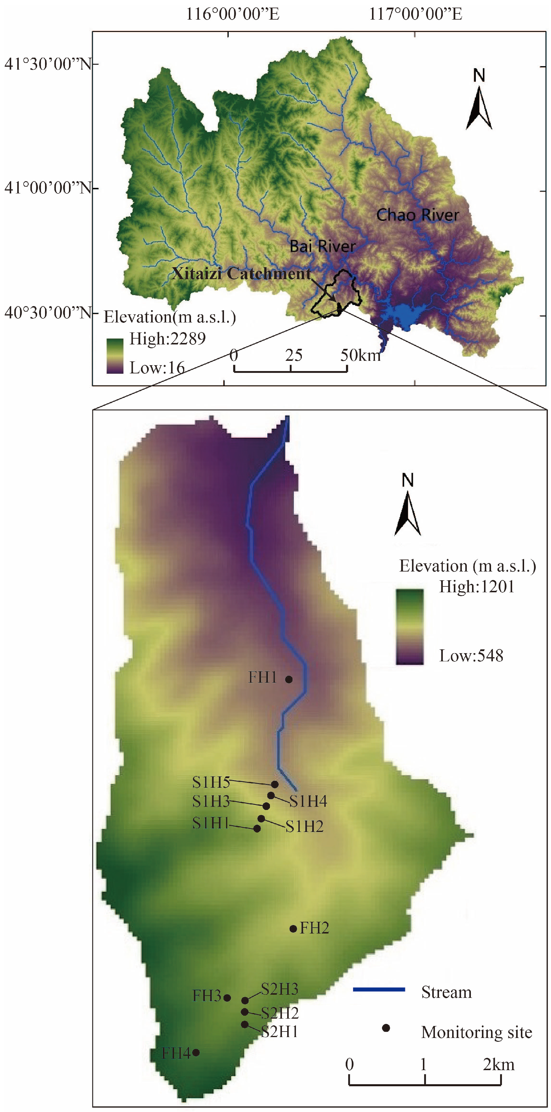
Observations were carried out at the Xitaizi experimental catchment (116°37′ E, 40°32′ N), which is located in the northern part of the municipality of Beijing, China, with an area about 7 km
2 and altitudes ranging between 550 m and 1200 m (
Figure 1). Local mean annual rainfall is 625 mm (1989–2013), with more than 80% of the rainfall amount occurring between June and September. Local mean annual temperature is 11.45 °C (1989–2013), and soils are frozen from late November to mid-March, when daily mean air temperature is continuously below 0 °C. The hillslope at this catchment is well covered by forest, which is composed mainly of
Larix gmelinii and
Populus davidiana, and the canopy coverage may reach 98% in summer (Source: SPOT, August 2013) when leaves are extensive. Soils at the hillslopes are not well developed, and the bedrocks are shallowly covered and occasionally exposed. Soil is commonly mixed with gravel, the size of which varies from millimeters to decimeters. Soil texture in the 0–60 cm depth varies from sandy loam to silt loam, with the content of clayey particles varying from 0.3% to 8.4% by weight.
In total, 12 sites were selected for observations in this catchment (
Figure 1). Four sites (FH1–FH4) were located in relatively flat areas, and the other 8 sites were distributed along two hillslopes, from high to low. At each site, TDR technique based CS616 probes (Campbell Scientific, Inc., Logan, MA, USA) with accuracy of ±0.025 cm
3/cm
3 were used to monitor the volume of water content in soils. They were deployed in layers within the top 60 cm or deeper, and the depth increments between adjacent probes were all 10 cm. Water content was continuously measured every 10 min, and the results were automatically recorded by CR1000 data loggers (Campbell Scientific, Inc., Logan, MA, USA). The dataset of volume water content within the top 60 cm obtained in unfrozen seasons (1 April 2015–31 October 2015) was analyzed, and time-series of soil moisture monitored by a probe were averaged into daily means as a preprocessing factor.
4. Results and Discussion
4.1. Relationship between Spatial Mean and Spatial Variance
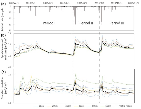
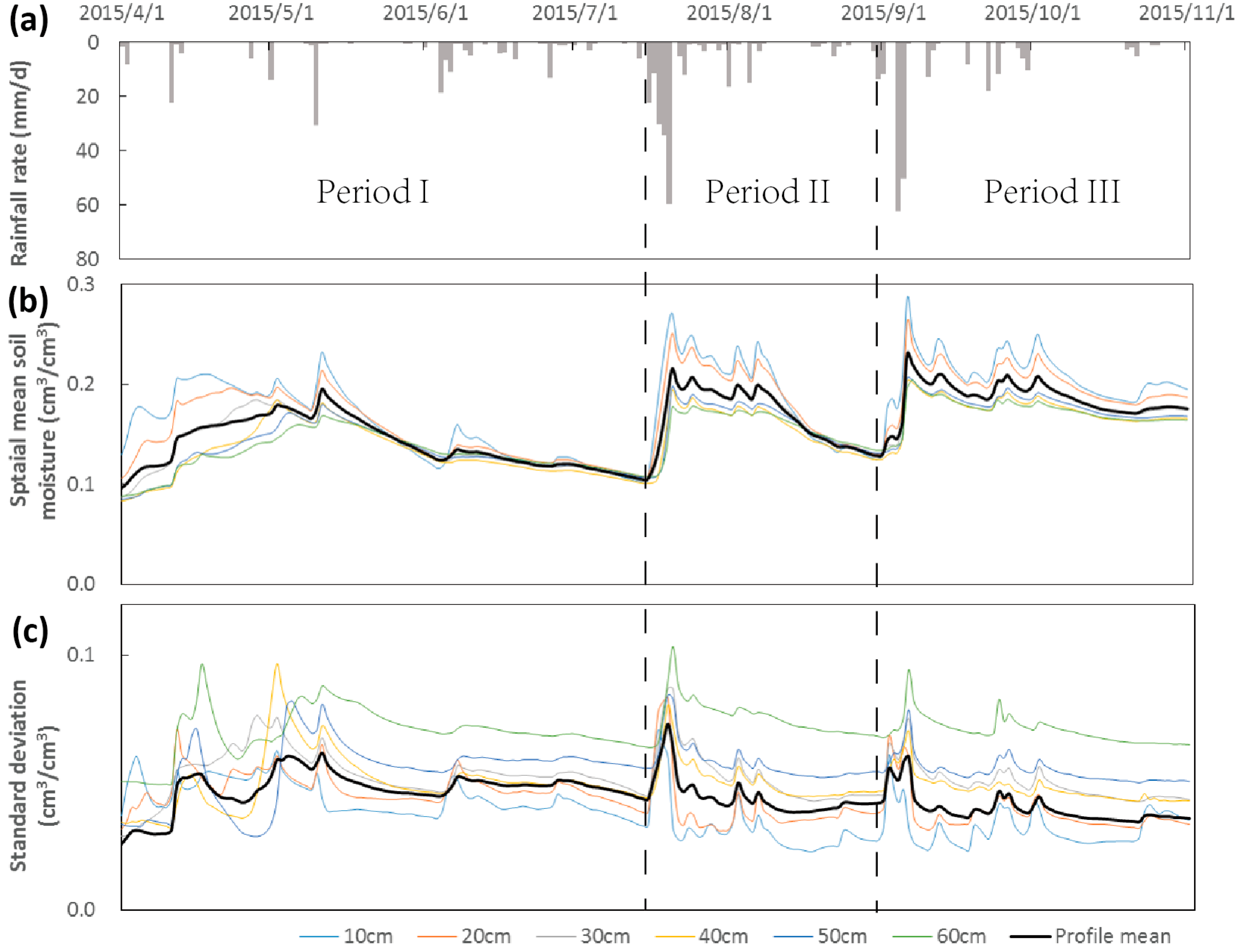
Figure 2 shows that spatial mean and standard deviation varied almost synchronously and in cyclic patterns. Based on the fluctuations of spatial mean, the whole monitoring period could be divided into three periods.
Period I covered 1 April 2015 to 15 July 2015, with 117 mm of rainfall. Basically, the spatial mean increased continuously until mid-May, and peaks of all depths were reached almost at the same time, despite some setbacks at some depths between rainfall events. While a total of 56 mm of rainfall occurred between 16 May 2015 and 15 July 2015, which was almost equal to that between 1 April 2015 and 15 May 2015, the spatial mean at all depths decreased continuously during this period. It increased occasionally during some heavy rains (e.g., around 1 June 2015), but was not enough to change the trend of decrease in the longer term. Temporal variation of standard deviation in this period was more complicated than that of spatial mean. It fluctuated more abruptly and more notably, especially during the ascending period of spatial mean (e.g., in mid to late April). Nonetheless, standard deviation generally showed an increasing trend in April and peaked in mid-May, one or two days earlier than the spatial mean. The decreasing period of standard deviation was smoother and generally kept pace with the spatial mean.
Period II and Period III could be divided by the date 31 August 2015, when the spatial mean reached a minimal value. Temporal variation of soil moisture and relevant standard deviation also showed similar variations in the two periods. Peaks of both spatial mean and standard deviation were reached during or right after the heaviest rain, and the two then declined continuously with small fluctuations.
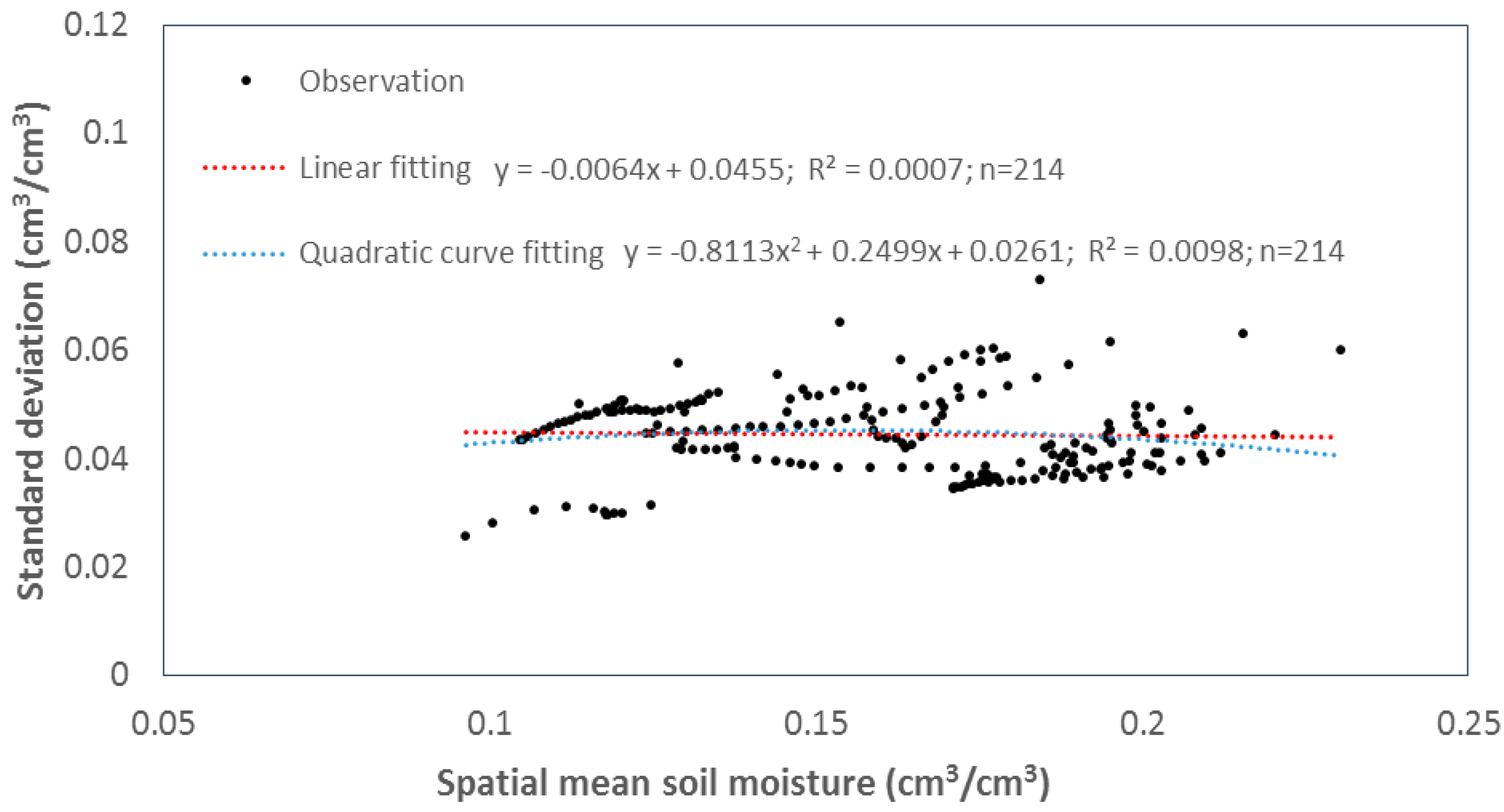
Although spatial mean and standard deviation varied synchronously, no significant correlation was found between the two statistical variables. As shown in
Figure 3, the linear correlation coefficient (R
2) between spatial mean and standard deviation of profile mean soil moisture was only 0.0007, and the non-linear correlation coefficient was not much higher, while the correlation coefficients between the two statistical variables of each depth were even lower.
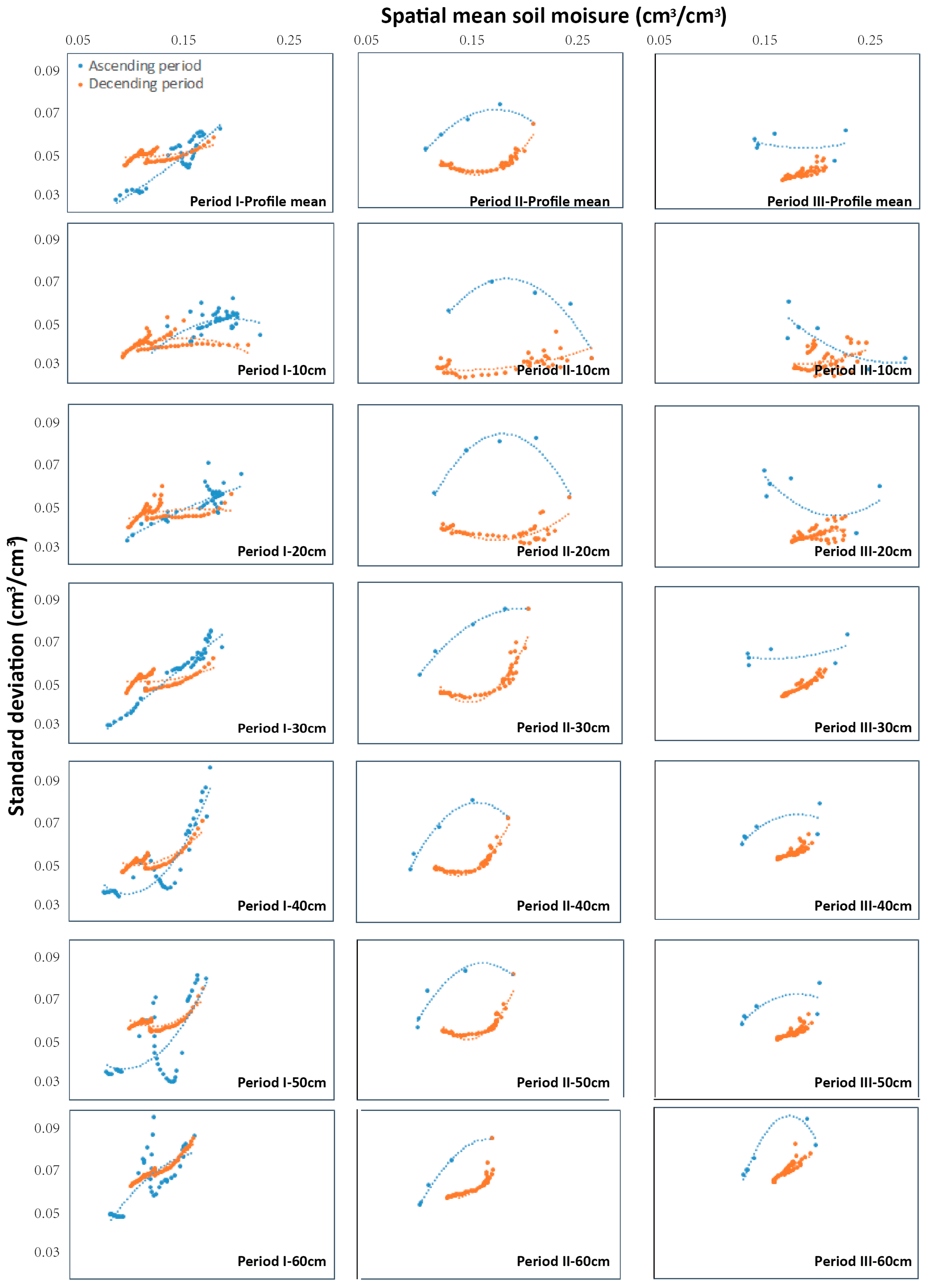
In the next step, the relationships between spatial mean and spatial variance of soil moisture in the three periods were examined individually (
Figure 4). The analysis showed that relationships between the two were not one-to-one mappings. On the contrary, at a given spatial mean, standard deviation obtained during the ascending period of the spatial mean was normally higher than that obtained during the descending period, resulting in clockwise hysteresis.
During the ascending period, standard deviation was positively correlated and frequently showed an upward convex relationship with the spatial mean, indicating standard deviation was about to fall when the spatial mean exceeded a critical point, although this critical point varied among different depths and different periods. During the descending period, standard deviation fell rapidly as the spatial mean decreased from its peak, but this falling tended to be slower as decrease of the spatial mean continued. Standard deviation may tend to increase again when the spatial mean decreases below some point, resulting in downward convex correlations between the two.
A quadratic curve was applied to fit the relationship between standard deviation and spatial mean during the ascending and descending periods individually (
Figure 4).
where
and
are the spatial mean and standard deviation, respectively; and
,
, and
are fitted parameters.
R2 of all fitting curves are listed in
Table 1, and 36 out of 42 fitting curves showed significant correlations with a significance level of 0.05. Among the 36 well-fitted curves, values of
were mostly negative during the ascending period (15 out of 21), and were positive during the descending period (17 out of 21). This pattern indicated that relationships between standard deviation and spatial mean were potentially all upward convex during the ascending period, and were potentially all downward convex during the descending period.
Temporal variation of spatial variance and the hysteresis of the relationship between the spatial mean and spatial variance should have been generated by the spatially heterogeneous water fluxes in soil. As a matter of fact, soil moistures at flat areas (FH1–FH4) were continuously among the highest, while those at the steepest slope (S1H1–S1H5) were always among the lowest. Moreover, at antecedently wetter sites, water infiltrated more and faster into soils during rainfall events [
39]. In this case, at an early state of rain, an increase in the spatial mean was attributed mainly to soil moisture increase at antecedently wetter sites, resulting in higher spatial variance. However, the increase rate of soil moisture at wetter sites tended to decrease as rain continued, due to the occurrence of subsurface flow and percolation, while soil moisture at drier sites kept increasing, thus leading to higher spatial mean but lower spatial variance. Observation showed that soil moisture at wetter sites decreased faster in a post-rain period, which could also be ascribed to stronger subsurface flow and percolation. Meanwhile, the root uptake may also impose a “homogenizing” effect on soil moisture during this period [
40], with spatial variance decreasing with the reduction of spatial mean.
Rosenbaum et al. (2012) [
41] also studied the clockwise hysteresis of the relationship between spatial mean and spatial variance, and concluded that this effect was more likely to occur for intense rain. The same observation occurred in this study, as rainfall during the three periods was 117 mm, 248.3 mm, and 208.3 mm, respectively, and was temporally more concentrated in Period II and Period III than in Period I. It can easily be concluded from
Figure 4 that the hysteresis was most clearly present in Period II; while in Period III, although the fitted curves failed to compose a circle in several diagrams, spatial variances during ascending periods were mostly higher than those during descending periods.
4.2. Contributions of Temporal Dynamic and Time-Invariant Factors
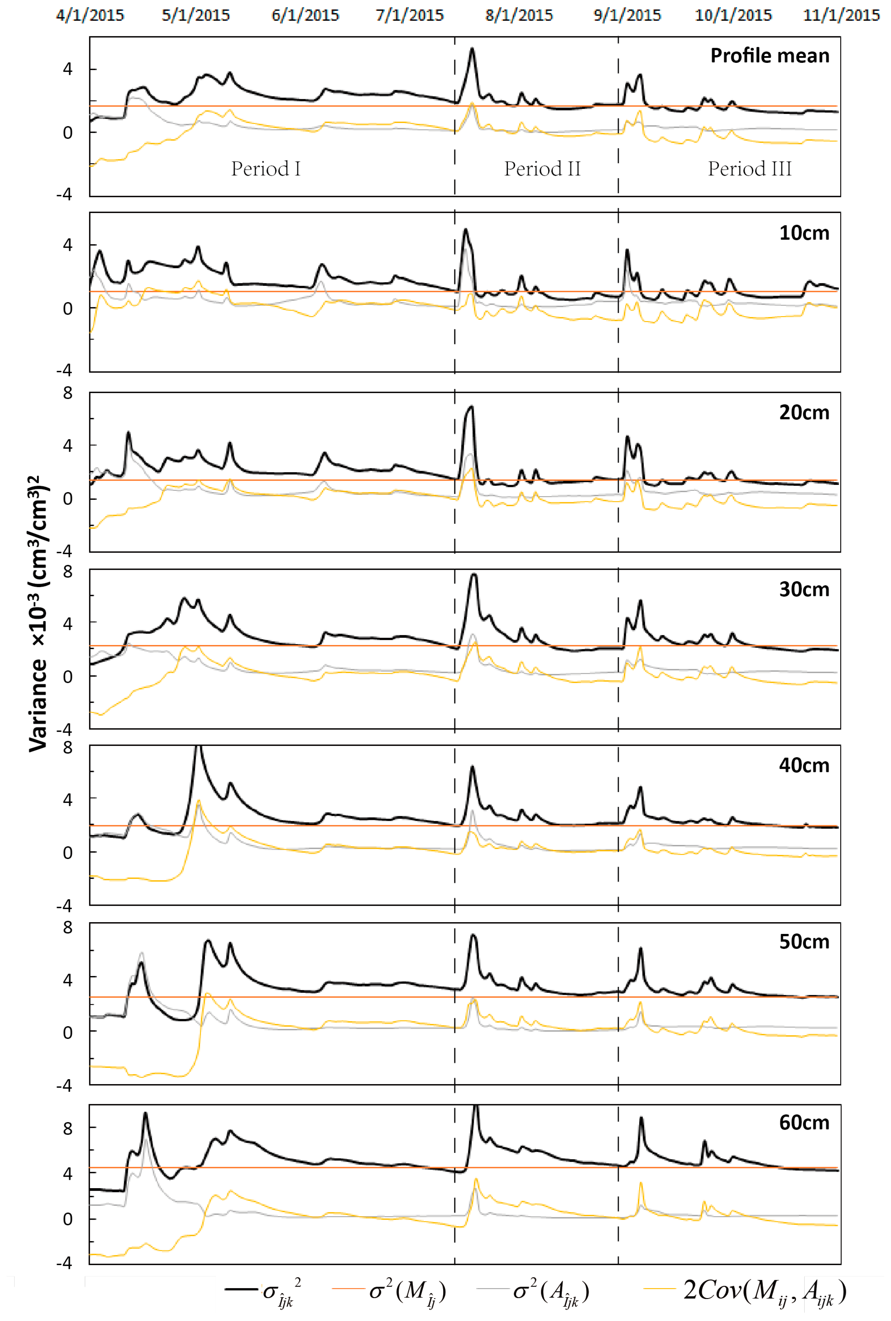
Obviously, temporal variation of
was contributed by the sum of
and
.
Figure 5 shows that temporal variation of the two generally followed the same pace of
, and major peaks of
(e.g., around 22 July 2015 and 5 September 2015) were captured by both contributors. Individual examination of the two indicated that
was in better correlation with
. Small fluctuations of
were all captured by
, and, moreover, the ascending process of
in April as well as the descending processes of
in each of the three periods were all synchronized by
, while
was less sensitive to fluctuations of
and remained largely constant during descending processes of
.
Given the notable temporal variation of , and , instantaneous contributions of each component varied highly across the monitoring period. Specifically, varied from less than 20% to more than 300%, with its temporal mean ranging between 81% and 94% at the 6 depths. The range of was between 1% and 181%, and its temporal mean was between 12% and 31% at each depth, while was more likely to be negative, since its temporal mean varied from −5% to −21% and could be as low as −309%, although its highest value was 41%.
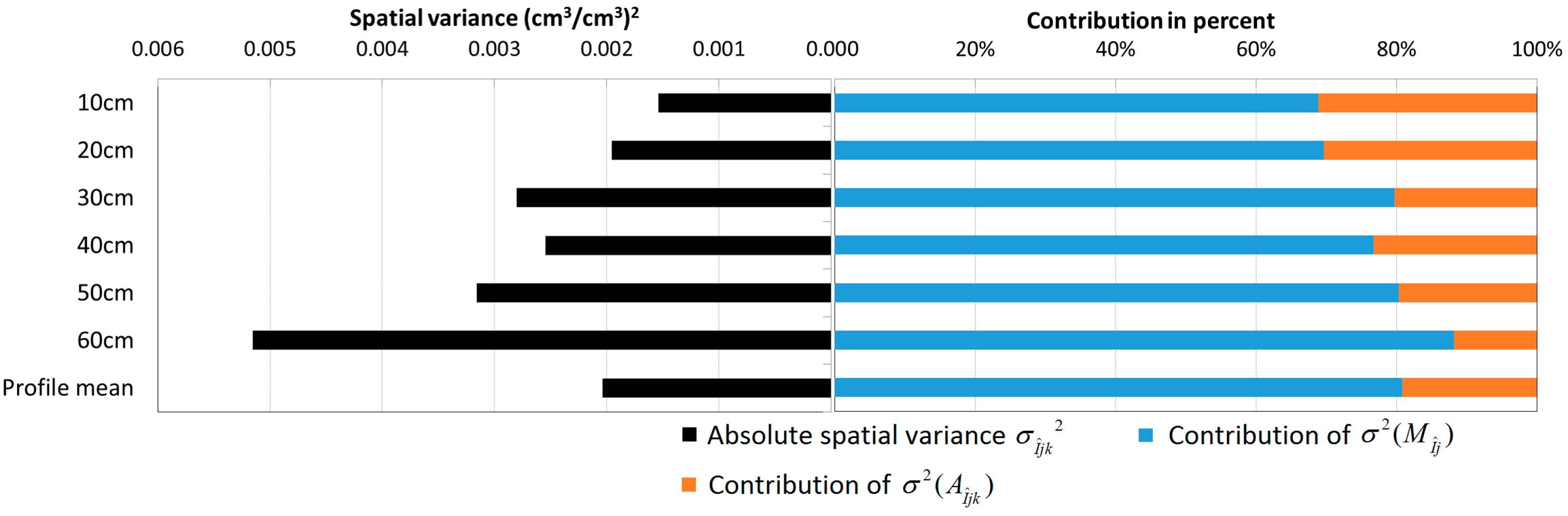
From another perspective, temporal means of
as well as those of its components were calculated and are shown in
Figure 6. Total variance
increased along with depth, from 0.0015 (cm
3/cm
3)
2 at 10 cm to 0.0052 (cm
3/cm
3)
2 at 60 cm, except for a small setback at 40 cm. Meanwhile, the temporal mean of
also increased from 0.001 (cm
3/cm
3)
2 to 0.0045 (cm
3/cm
3)
2, increasing its contribution from 68.9% to 88.2%. Temporal means of
were less varied among the depths, and ranged within 5.8 × 10
−4 ± 5.2 × 10
−5( cm
3/cm
3)
2, leading to a decrease in its contribution from 31.1% to 11.8% with depth. The temporal mean of the covariance term can be decomposed by Equation (19):
where
is the temporal mean of the covariance term. Since the temporal sums of both the temporal anomaly (
) and the spatial mean temporal anomaly (
) are zero, the result of
is inevitably zero. Consequently, the temporal mean of the covariance term is mathematically zero and invisible in
Figure 6.
4.3. Rank Stability of Monitoring Sites
Ranks of all the 12 sites obtained from the two strategies mentioned in
Section 2.3 are displayed in
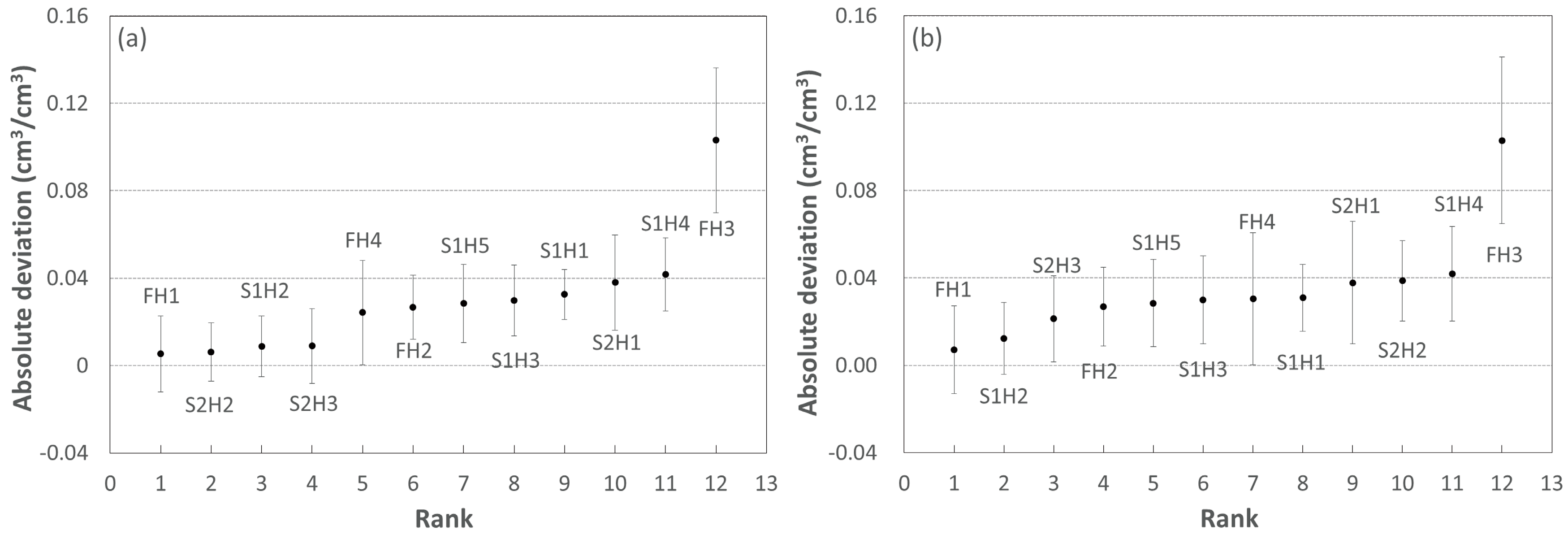
Figure 7. One may note some similarities between the two sets of ranks. For example, the profile mean and profile distribution of soil moisture at FH1 were both closest to relevant spatial means, while those at S1H4 and FH3 were always the ones that deviated the most. In addition, temporal mean absolute deviation of the sites that ranked from 1 to 11 in the two strategies all ranged between 0 and 0.04 cm
3/cm
3, but at the same time there were large gaps between those of S1H4 and FH3, with those of the latter always more than double those of the former. Nevertheless, the remaining 9 sites all obtained different ranks in the two strategies, with S2H2 being the one that varied the most. Temporal mean absolute deviation of S2H2 increased from less than 0.007 cm
3/cm
3 in Strategy I to 0.038 cm
3/cm
3 in Strategy II, and rank of this site consequently changed from 2 to 10.
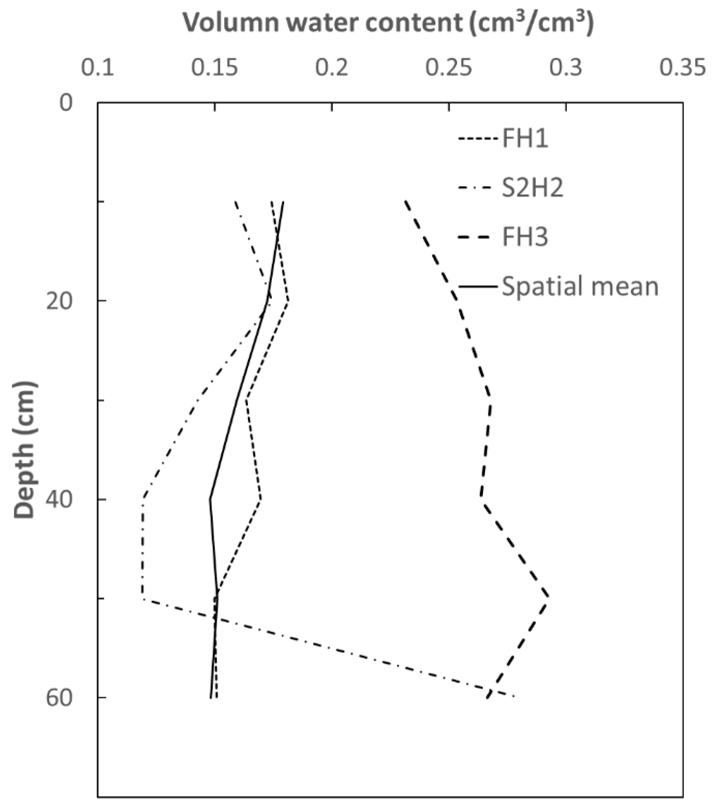
Soil moisture profiles shown in
Figure 8 could be an explanation of the performances of the sites in both strategies. Since soil moistures at all depths at FH3 were all higher than those of the profile mean,
(see Equation (8)) at this site was likely to be positive all through the profile, thus
(see Equation (11)) and
(see Equation (14)) were likely to be equal, consequently leading to equal results of temporal mean absolute deviation in the two strategies (
Figure 7). On the contrary, at S2H2,
could be both positive and negative, and thus
was normally less than
. As a result, although profile mean soil moisture at this site was close to the spatial mean, its profile distribution deviated much farther from the spatial mean.
Comprehensive analysis by the Spearman test showed that it was the similarity rather than the difference that played a dominant role between the ranks obtained from the two strategies, since the correlation coefficient between the two was 0.706 (Equation (17)), which was higher than the critical value (0.506) at significance level of 0.05.
As Brocca et al. (2009) stated [
29], a low value of
is generally a characteristic of the temporal “stable” site, and S1H1 was supposed to be the most temporal stable site in both strategies given its lowest values of
. From another perspective, we examined the ranks of sites in each of the three periods, and a Spearman test showed that ranks of sites through the whole monitoring period were significantly correlated with those of Period I–Period III, in both strategies (
Table 2), whereas ranks obtained in Period II and Period III were not significantly correlated. Interestingly, it was FH3, the site with the highest value of
, that kept its rank all through the monitoring period, in both strategies.
4.4. Influence of Samping Strategy on Spatial Variatbility
Western et al. (1998) [
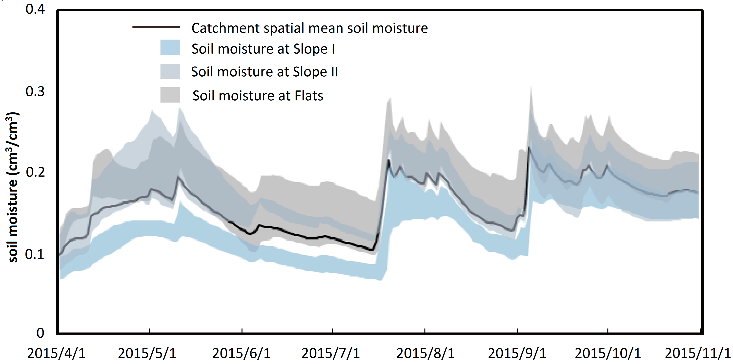
15] reported that soil moisture could be spatially organized, since sites that were close to each other or with similar terrain indices may have similar water content. In this study, the 12 monitoring sites could easily be categorized into three groups based on topography. As shown in
Figure 9, soil moistures were also likely to be spatially organized in this study area. Soil moistures at Slope I were always lower than the spatial mean, but those of the other two groups were mostly higher than the spatial mean through the monitoring period. One may also note that the in-group standard deviations of Slope I and Slope II were much smaller than those of all 12 sites (Compared with
Figure 2), while the in-group standard deviations of Flats were higher and closer to that of all 12 sites.
Moreover, spatial deviation obtained by Equation (2) could be separated into two parts according to the decomposition equation of deviation, and relevant components were (i) in-group variance: spatial variance of soil moisture within each group of sites; and (ii) inter-group variance: variance between the means of each group:
where
,
and
are number of sites in each of the three group; and
,
and
are mean soil moisture within each group, respectively.
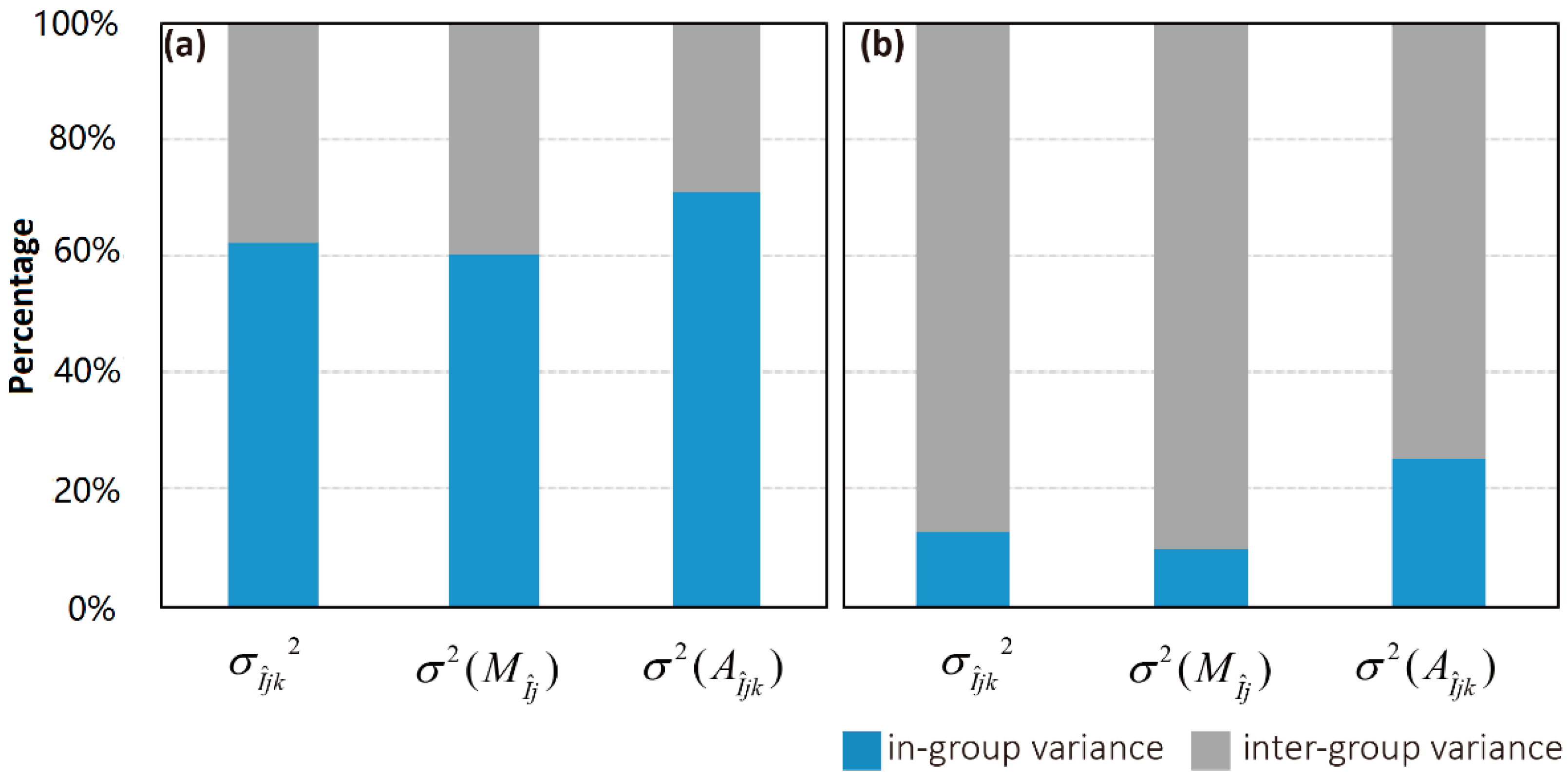
Taking the spatial variance of profile mean soil moisture as an example, temporal mean contributions of in-group and inter-group variances are shown in
Figure 10, with the component
ignored. In-group variance contributed more than 60% of the total variance when the 12 sites were separated into three groups, and also dominated the contribution in both
and
. However, if the 4 sites on Flats (FH1–FH4) were not regarded as a group, contributions of in-group variance generally declined to close to or lower than 20%. This finding suggested that soil moisture differences within the group of Flats (FH1–FH4) contributed more than 40% of the areal spatial variance, which was much higher than that of the other two groups combined. Thus, it was confirmed that soil moistures at Slope I and Slope II were spatially organized, while soil moistures at FH1–FH4, which were located far from each other, were less close.
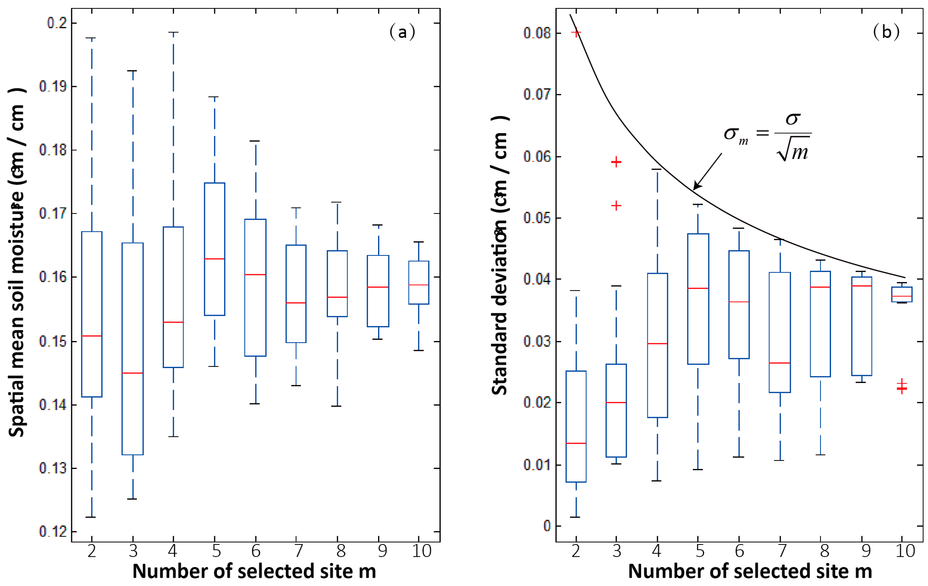
Further, in order to evaluate the influences of site selection on estimations of spatial mean and spatial variance,
sites (
) were randomly picked from the 12 monitored sites, and it was assured that each site was picked no more than once in each selection. The selection process was repeated 20 times, and temporal mean of spatial mean soil moisture as well as spatial variance are shown in
Figure 11. Estimated spatial mean was highly uncertain when only a small number of sites was selected, but this uncertainty would diminish with
, and the estimations tended to converge at the one that was estimated by all 12 sites (0.16 cm
3/cm
3). Variation of estimated standard deviation would also diminish with
. In principle, the uncertainty of spatial mean (
) was expected to decrease with
if the mean soil moisture could be estimated from multiple measurements located randomly. Further, in the idealized case where the observations were completely independent, the standard deviation was given by [
42]:
where
is standard deviation of individual site.
Standard deviation obtained by all the 12 sites was assumed to be the “true” value, and the “true” value of standard deviation when a different number of sites were selected should follow the black curve in
Figure 11b. However, all the estimated standard deviations were lower than the relevant “true” value, and the curve of “true” values was close to the upper limits of these estimations, rather than the mean or median values. Therefore, the spatial organization of soil moisture may result in non-independent samplings, and a small number of sampling sites would probably lead to underestimated spatial variability of soil moisture.
5. Conclusions
Spatial mean and spatial variance of soil moisture in the studied forest catchment varied almost synchronously and basically in three cyclic patterns during the monitoring period from 1 April 2015 to 31 October 2015. Spatial variance increased with spatial mean during rainfall, but it tended to decrease as spatial mean exceeded a critical point; while during the descending of soil moisture, spatial variance declined simultaneously but tended to increase as spatial mean decreased below some point. The spatial mean-variance relationship during the ascending and descending periods of spatial mean could be well-fitted by upward and downward convex quadratic curves, respectively, indicating possible clockwise hysteresis of this relationship.
Temporal anomalies of the spatial variance were deduced by temporal dynamic rainfall and other water fluxes. Results showed that all through the monitoring period, contributions of time-invariant factors on total spatial variance increased from 68.9% to 88.2% with depth. Given the dominant contribution of the time-invariant factor, the monitored 12 sites showed temporally stable ranks.
However, it was also noted that soil moisture was spatially organized and may lead to non-independent samplings. Analysis showed that the estimations were highly dependent on the monitoring sites, and a small number of sampling sites would probably lead to underestimated spatial variability of soil moisture.


