Review

Spatiotemporal Variability of Wildland Fuels in US Northern Rocky Mountain Forests

Missoula Fire Sciences Laboratory, Rocky Mountain Research Station, US Forest Service, 5775 Highway 10 West, Missoula, MT 59808, USA
Forests 2016, 7(7), 129; https://doi.org/10.3390/f7070129
Submission received: 3 May 2016 / Revised: 1 June 2016 / Accepted: 12 June 2016 / Published: 27 June 2016

Abstract

:
Fire regimes are ultimately controlled by wildland fuel dynamics over space and time; spatial distributions of fuel influence the size, spread, and intensity of individual fires, while the temporal distribution of fuel deposition influences fire’s frequency and controls fire size. These “shifting fuel mosaics” are both a cause and a consequence of fire regimes. This paper synthesizes results from two major fuel dynamics studies that described the spatial and temporal variability of canopy and surface wildland fuel characteristics found in US northern Rocky Mountain forests. Eight major surface fuel components—four downed dead woody fuel size classes (1, 10, 100, 1000 h), duff, litter, shrub, and herb—and three canopy fuel characteristics—loading, bulk density and cover—were studied. Properties of these fuel types were sampled on nested plots located within sampling grids to describe their variability across spatiotemporal scales. Important findings were that fuel component loadings were highly variable (two to three times the mean), and this variability increased with the size of fuel particles. The spatial variability of loadings also varied by spatial scale with fine fuels (duff, litter, 1 h, 10 h) varying at scales of 1 to 5 m; coarse fuels at 10 to 150 m, and canopy fuels at 100 to 600 m. Fine fuels are more uniformly distributed over both time and space and decayed quickly, while large fuels are rare on the landscape but have a high residence time.

1. Introduction

Fire regimes are created by the interaction of bottom–up and top–down controls [1]; bottom–up controls, such as vegetation, topography, and disturbance history, often dictate fire spread, intensity, and severity at fine scales, while coarse scale, top–down controls, such as climate and weather, dictate fire frequency, duration, and synchrony [2]. Of all bottom–up controls, wildland fuels are important because they govern most of fire’s combustion processes [3]. The spatial and temporal variability of wildland fuel directly impacts fire regimes which, in turn, has major implications for fire management [4]. Landscape patches that have minimal fuels, such as recently treated or burned areas, form fuel breaks that may limit growth, reduce intensity, and minimize severity for future fires [5]. This self-organizational property of wildland fire is incredibly important in predicting future fire dynamics under climate change [6,7]. Fire and fuel management should use the changing fuel mosaic to develop management plans that effectively integrate wildfires, controlled wildfires, prescribed fires, and fuel treatments to minimize firefighting costs and maximize ecosystem resilience while still protecting homes and people [8].
Wildland fuels are live and dead organic matter called biomass [9]. The forest fuelbed is vertically stratified into three fuel layers—ground, surface, and canopy fuels (Figure 1). Surface fuels are all biomass within 2 m above the ground surface. Ground fuels are all organic matter below the litter and above the mineral soil, which is called duff in most upland forests. Canopy fuels are the biomass above the surface fuel layer. Fuelbed layers are composed of finer-scale elements called fuel components, which are fuel types that are defined for specific purposes, mostly for fire behavior and effects prediction. A woody fuel type, for example, might be defined as a fuel component based on particle diameter size range (Table 1). The finest scale of fuelbed description is the fuel particle, which is a general term that defines a specific piece of fuel that is part of a fuel type or component of a fuelbed (Figure 1); a fuel particle can be an intact or fragmented stick, grass blade, shrub leaf, or pine needle. There are many physical properties that can describe fuel particles, such as specific gravity, heat content, weight, and shape, and statistical summaries of these particle properties are often used to quantify coarser fuel component properties. However, the fuel property most used in fire management is loading or amount of biomass per unit area (kg·m−2 in this paper).
An often overlooked feature of wildland fuelbeds is that they are always changing in space and in time; live and dead biomass are constantly being added, modified, and removed by various ecological processes, thereby changing particle, component, and layer properties [10]. The annual shed of leaves and small woody twigs from trees, for example, creates significantly different spatial distributions than the infrequent toppling of tree boles to create logs or coarse woody debris (CWD). As a result, wildland fuel landscapes can be thought of as shifting mosaics of hierarchically intersecting fuel characteristics [9]. This dynamic and complex character of fuelbeds across space and time is responsible for the great variability found in wildland fuel characteristics [11,12,13] and is perhaps the single most important concept to understand in fire management today because it influences strategic fuel management considerations such as fuel treatment longevity and effectiveness, fire return intervals, and smoke potential [9].
Numerous ecological processes influence fuel dynamics, but four are particularly important in controlling spatial and temporal distributions of wildland fuels—vegetation development, deposition, decomposition, and disturbance—the four “Ds” [9]. Wildland fuels accumulate as a result of the establishment, growth, and mortality of vegetation (development). Rates of biomass accumulation, often called productivity, are dictated by the interactions of the plant species available to occupy a site and the site’s physical environment (e.g., climate, soils, and topography) [14]. Over time, portions of living biomass are shed or die and get deposited on the ground to become dead surface fuels or necromass. Below- and above-ground necromass is eventually decomposed by microbes and soil macrofauna. Disturbances, such as fire, insects, and disease, act on living and dead biomass to change the magnitude, trend, and direction of fuel dynamics in space and time. These four fuel processes interact, but they are often influenced by different environmental factors depending on the ecosystem. In wildland fuel science, for example, many assume fuels are closely related to vegetation characteristics [15], but this would be true only if the first two processes (development and deposition) were considered thereby ignoring the role of decomposition and disturbance in fuelbed development.
The landscape ecology of wildland fuels is the interaction of the above processes across multiple space and time scales to create the shifting mosaics of fuel conditions [16]. Understanding the spatial and temporal dynamics of fuels may provide a better grasp of the impact of various wildland fuel management activities on fuel properties [17] and it also might help explain unexpected fire behaviors and effects (e.g., [18]). It may also aid in developing effective fuel applications that integrate spatial variability in their design such as new fuel classifications, sampling methods, and geospatial data [9]. Patterns of fuel characteristics will be important inputs to the fire effects and behavior models of the future [18,19].
Few have explored spatial and temporal relationships of the wildland fuels. Reich et al. [20] evaluated the spatial variability of several fuel components over a large landscape in the US Black Hills and found that the variability was governed by topography and vegetation. Hiers et al. [21] measured small-scale variations in surface fuel using LiDAR and found that fuelbed depths become spatially independent after small distances (~0.5 m2). Spatial variability of grasslands have been described in the context of population dynamics and restoration potential but have not been related to fuel characteristics [22]. Theobald [23] found that while fine scale variation in fuels dictated fire behavior, the distribution of CWD dictated germination in longleaf pine ecosystems. Kreye et al. [24] described the spatial structure of duff near tree boles using Moran’s I and found duff depth had high spatial correlations at short distances (<1 m). While some studies described fuel distributions across landscapes [25,26], few have actually quantified the variability of fuel properties across space [19,27,28]. And, while many have identified fuel continuity as an important spatial characteristic of wildland fuels [29,30], few studies have addressed the structure of fuel spatial variation at landscape scales.
This paper is a synthesis of two long-term projects that were designed to understand the spatial and temporal dynamics of wildland fuelbeds. Spatial fuel characteristics were measured for eight fuel components (Table 1) in an extensive study called FUELVAR that assessed fuel component properties at various distances in a 1 km sampling grid installed in six US northern Rocky Mountain stands [11,16]. Temporal fuel dynamics were measured on 28 plots across the northern US Rocky Mountains over a period of 10–12 years to assess deposition and decomposition rates for five fuel components in the FUELDYN study (Table 1) [31,32]. While these two studies were not directly linked, many methods and analyses overlap, and as a result, the findings can be described in a similar context. In this paper, the two studies are used to demonstrate the variability and complexity of wildland forest fuelbeds over time and space.

2. Methods

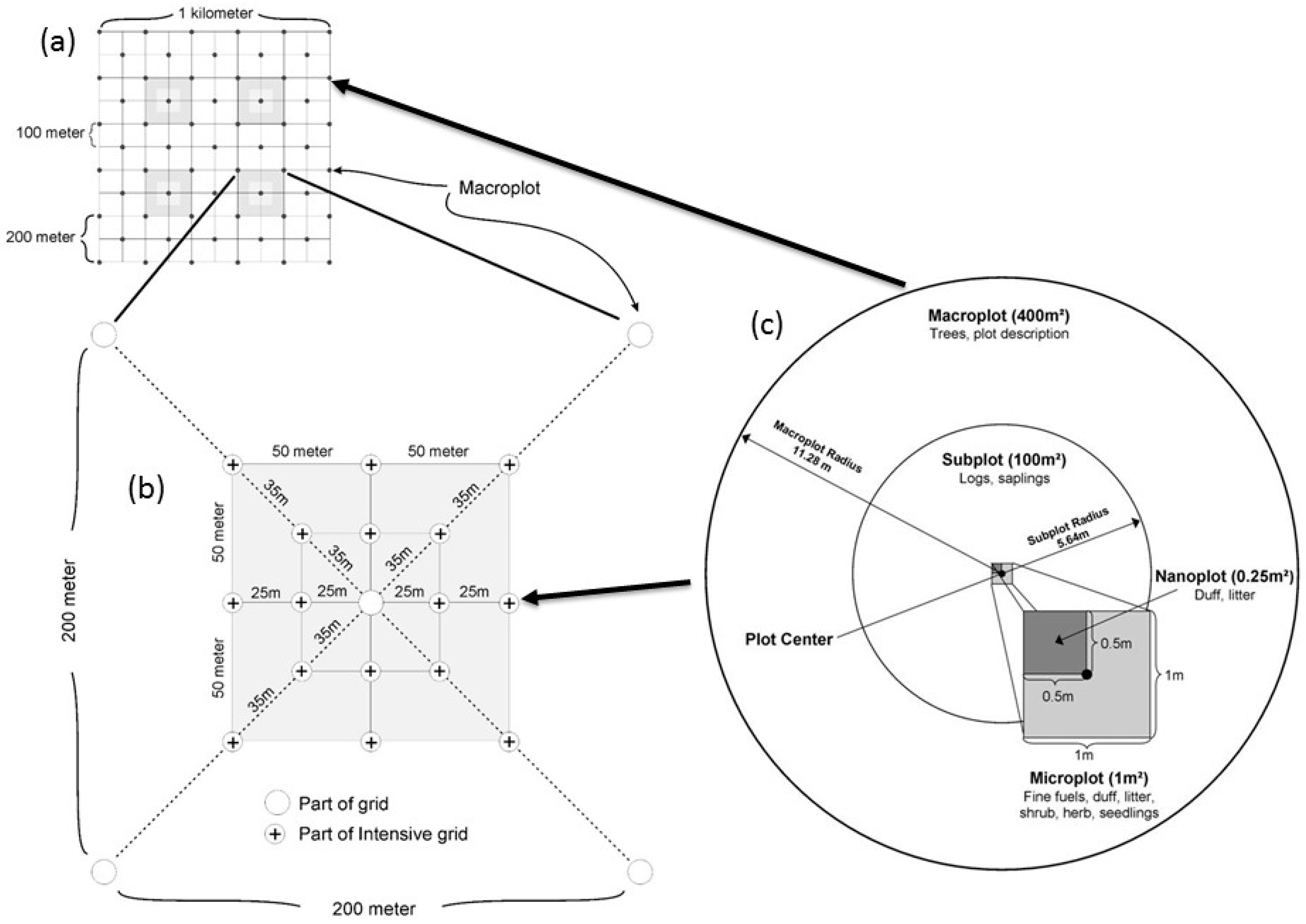
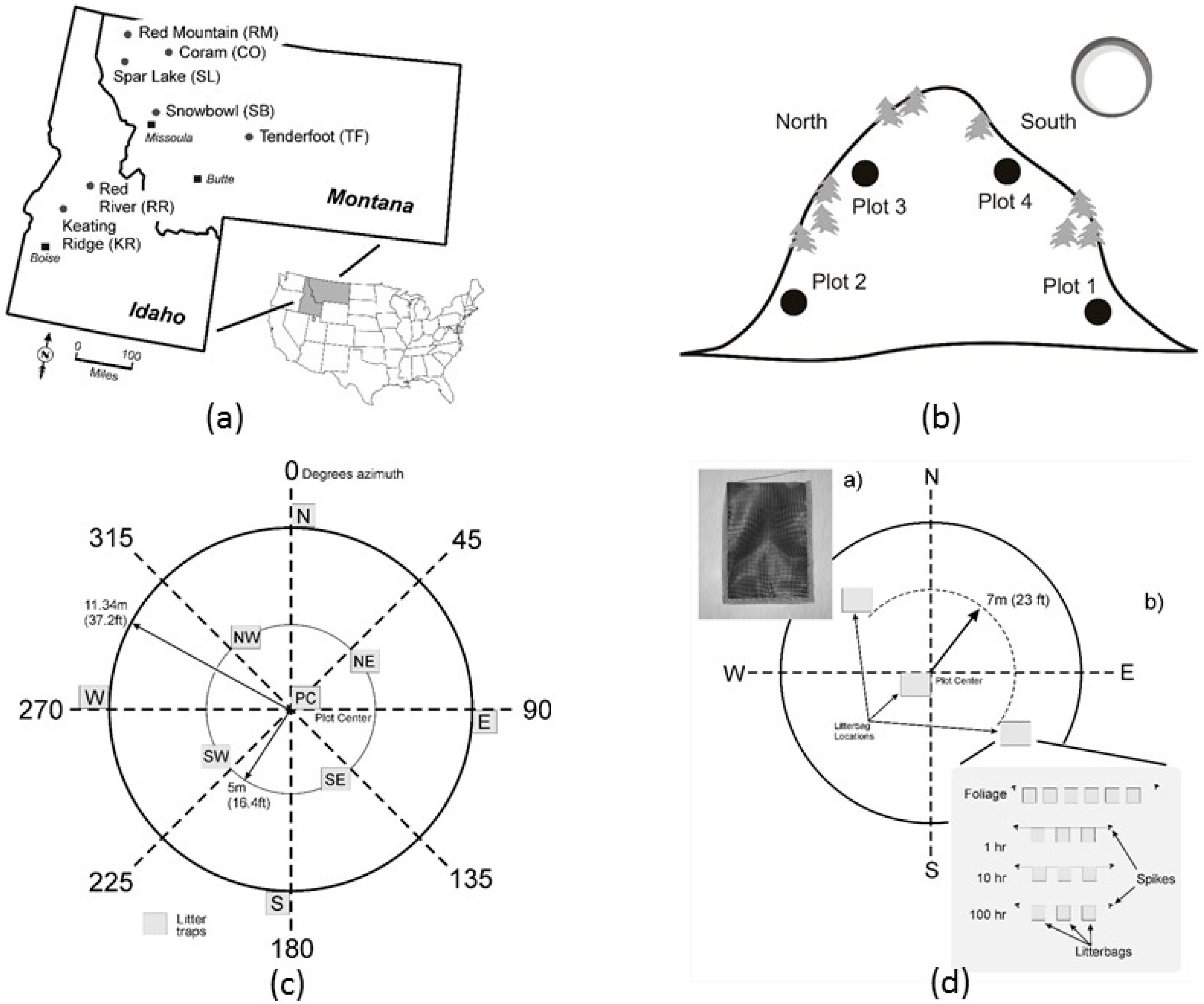
2.1. Spatial Methods

In the FUELVAR study, a nested grid design within a square 1 km2 area was installed in the center of six selected study sites [11] (Figure 2a). Sites sampled included a second-growth dry mixed conifer stand of ponderosa pine (Pinus ponderosa), Douglas-fir (Pseudotsuga menziesii), and western larch (Larix occidentalis) that had been thinned, a ponderosa pine-Douglas-fir stand that had been prescribed burned, a lodgepole pine (Pinus contorta) stand with a history of non-lethal surface fires, a pinyon pine (Pinus edulis) and juniper (Juniperus occidentalis) woodland, a ponderosa pine savanna, and a sagebrush grassland. Sides of the sampling grid were oriented along the four cardinal directions. Transects were established at each corner and at 100-m intervals along each grid side (Figure 2a). Sampling was intensified around four central grid points to increase the number of distances between sample points by installing a nested sampling grid of 16 additional sampling points centered around one of the four grid points using a 100-m square (eight sampling points) and 50-m square (another eight points) design (Figure 2b). These additional sampling points were placed at the corners and side mid-points for the two nested squares. This intensive grid provided the additional distances, including 25, 35, 50, and 100 m.
A 400-m2 circular macroplot was established at each grid sample point for sampling trees greater than 10 cm DBH (diameter breast height) and canopy cover (Figure 2c). Using the same sample point as plot center, we installed a 100-m2 circular subplot on which we sampled logs (woody fuel particles greater than 8 cm diameter) and sapling trees (trees greater than 1.37 m tall and less than 10 cm DBH). We then centered a 1-m2 square microplot over the grid sampling point, within which we measured shrub, herb, and fine woody (wood fuel particles less than 8 cm diameter; twigs and branches) fuel characteristics. Last, a 0.25-m2 (50 by 50 cm) square nanoplot was installed in the northwest corner of the microplot to measure duff and litter fuels.
Spatial variability of the measured fuel loadings of each component (Table 1) was described using semi-variograms; a descriptive technique that graphically represents the spatial continuity and spatial autocorrelation of a spatial data set [33,34]. Semi-variogram range, the distance where the variance curve first flattens, is important in landscape ecology because it represents the spatial scale at which the entity of concern is best described in space, often called the inherent patch size [35].

2.2. Temporal Methods

In 1993, a set of litter traps were installed on four plots on each of two sites in western Montana to parameterize and validate two ecosystem models [31]. Then, in 1995, four new sites were established along elevational and aspect gradients within the larger US Northern Rockies study area (Figure 3a). Plots were established only in mature stands that had no evidence of disturbance. Forest types represented by these sites include stands dominated by ponderosa pine, Douglas-fir), western red cedar (Thuja plicata), subalpine fir (Abies lasiocarpa), and whitebark pine (Pinus albicaulis). In 1996, a seventh site was established in the ubiquitous lodgepole pine ecosystem that occurs east of the Continental Divide (Figure 3a).
Four plots were established at each site established along major topographic gradients of elevation and aspect to capture the diversity of the important direct environmental gradients such as productivity, moisture, and temperature (Figure 3b). A number of topographic, vegetation, and ecosystem characteristics were measured on the 0.1 acre (0.04 ha) circular plots, and then an inventory of all trees within plot boundaries was conducted. A network of 30 m fuel transects to estimate fuel loadings for five fuel components was also used in this study.
At each plot, we installed nine 1 m by 1 m litter traps in the star pattern to collect fallen biomass (Figure 3c) but two were removed (NW, SE) after statistical analysis revealed they weren’t needed. Each plot was visited once a month during the snow-free periods of the year and all material in each trap was placed into heavy paper bags, transported to the laboratory, and the labeled bags were placed in an oven set at 90 °C for two to three days. The weight of each fuel component was recorded to the nearest 0.01 g along with the date, site, plot, and trap information written on the bag. A small sample of the dried material was set aside for the decomposition experiment. We measured litterfall in these traps for 10–12 years depending on the site.
Litter bags were used to estimate the rate of decay for four fuel components of freshly fallen foliage, twigs, branches, and large branches [31]. Approximately 100–150 g of the material taken from the litter traps was put into each bag and then the bag was sewn closed. Decomposition rates for logs and other canopy material were not measured because of limited time, lack of appropriate equipment, and incompatible methods. At each plot, three sets of three bags for the three fine woody fuel components (1, 10, and 100 h) and three sets of six bags for the foliage material were installed in the pattern shown in Figure 3d. Decomposition was measured over three years by taking one foliage bag from each wire set every 6 months and one woody bag from each woody fuel set every 12 months. The litter bags were then placed in paper bags, dried at 80 °C for 3 days, and then weighed to the nearest 0.01 g with the weight.
Two estimates of decomposition were calculated. A mass loss rate (percent year−1) was calculated from differences in bag weights over the three year period. Then, we estimated the decomposition parameter k in the Olson [36] equation using a linear mixed effects model whose form is as follows:
ln ( x i j x i 0 ) = ( k + b i ) t j + ε i j
where xij is the weight of the ith trap at time j (tj) and xi0 is the initial weight of the ith trap; bi is the random effect of trap i representing the deviation of the slope from the fixed effect for trap i; and εij are the random errors assumed to be independently distributed with a normal distribution.

3. Results

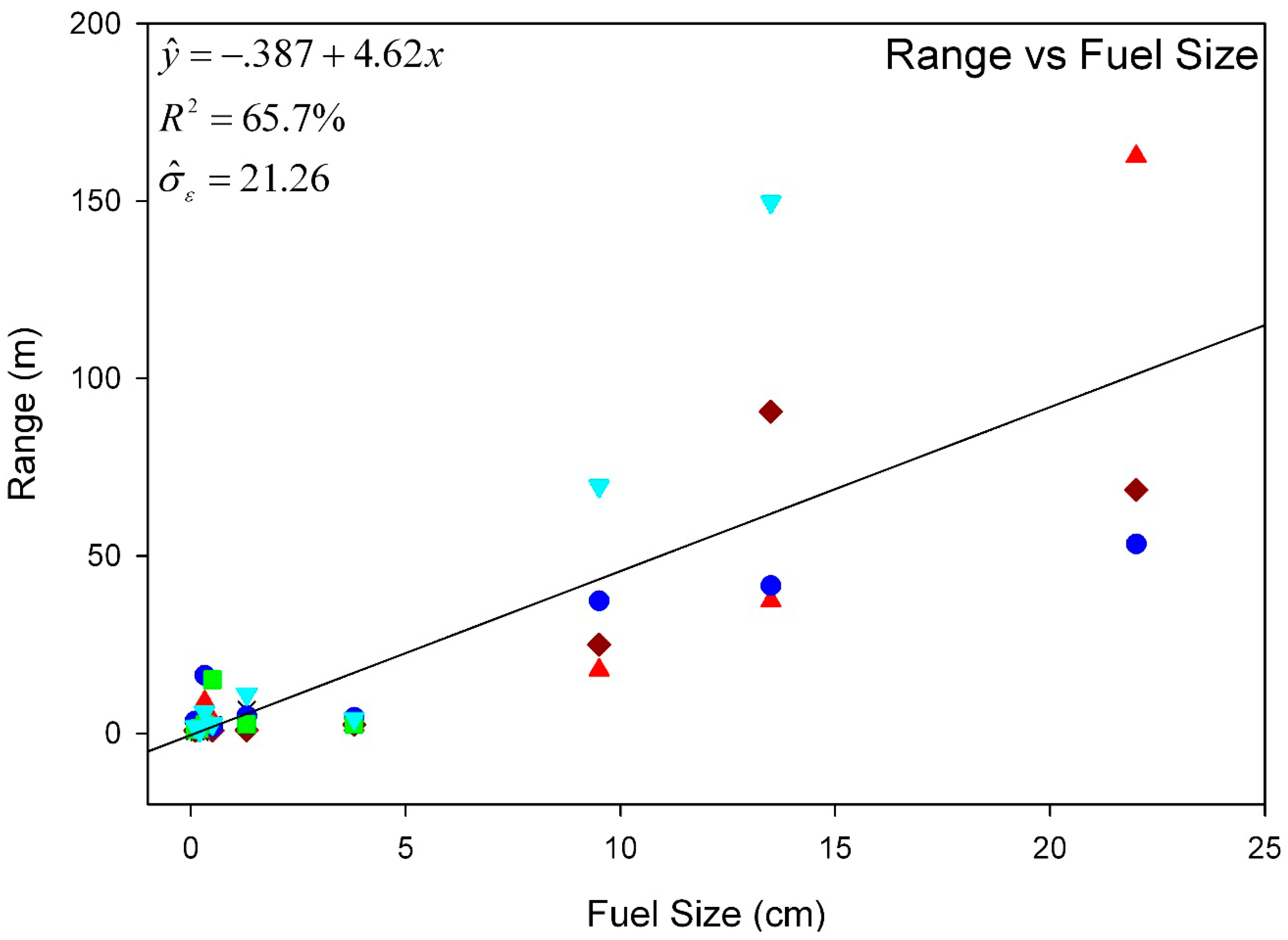
3.1. Spatial Dynamics

Using semi-variogram analysis, Keane, Gray and Bacciu [11] estimated the spatial scale of individual canopy and surface fuel components and found that the smaller the fuel component, the finer the scale of spatial distribution. Fine woody debris (FWD, Table 1) varied at scales of 1–5 m, depending on the size of fuel particle; CWD varied at 22–160 m; and canopy fuel characteristics varied at 120–600 m scales (Table 2). In fact, Keane, Gray, BacciuandLeirfallom [16] related fuel particle diameter with semi-variogram range and found that an increase in 1 cm in fuel particle diameter resulted in an increase of the range (inherent patch size) by 4.6 m (Figure 4). Results from the FUELVAR study showed that each fuel component has its own inherent spatial scale and that this scale varies by biophysical environment, vegetation structure and composition, and time since disturbance.
There were several other findings of the FUELVAR study that warrant mention. First Keane, Gray and Bacciu [11] found high variability in a number of fuel properties both across and within sites; coefficients of variation (variation expressed as a percent of the mean) exceeded 200% for loading of most woody fuel components and that variation was correlated with particle size (R2 = 0.6). They also found that this variability was not normally distributed, but instead, highly skewed (skewness statistic >2.0 for most components) because many microplots were missing fuel components. Next, Keane, GrayandBacciu [11] found that none of the surface fuel components were correlated with each other; correlation coefficients were <0.4 for the loading of all combinations of surface fuel components. Even more important was the fact that none of the surface fuel components correlated with canopy fuel components or numerous other stand characteristics, such as tree density, basal area, and tree diameter. Each fuel component was distributed independently of all other components.

3.2. Temporal Dynamics
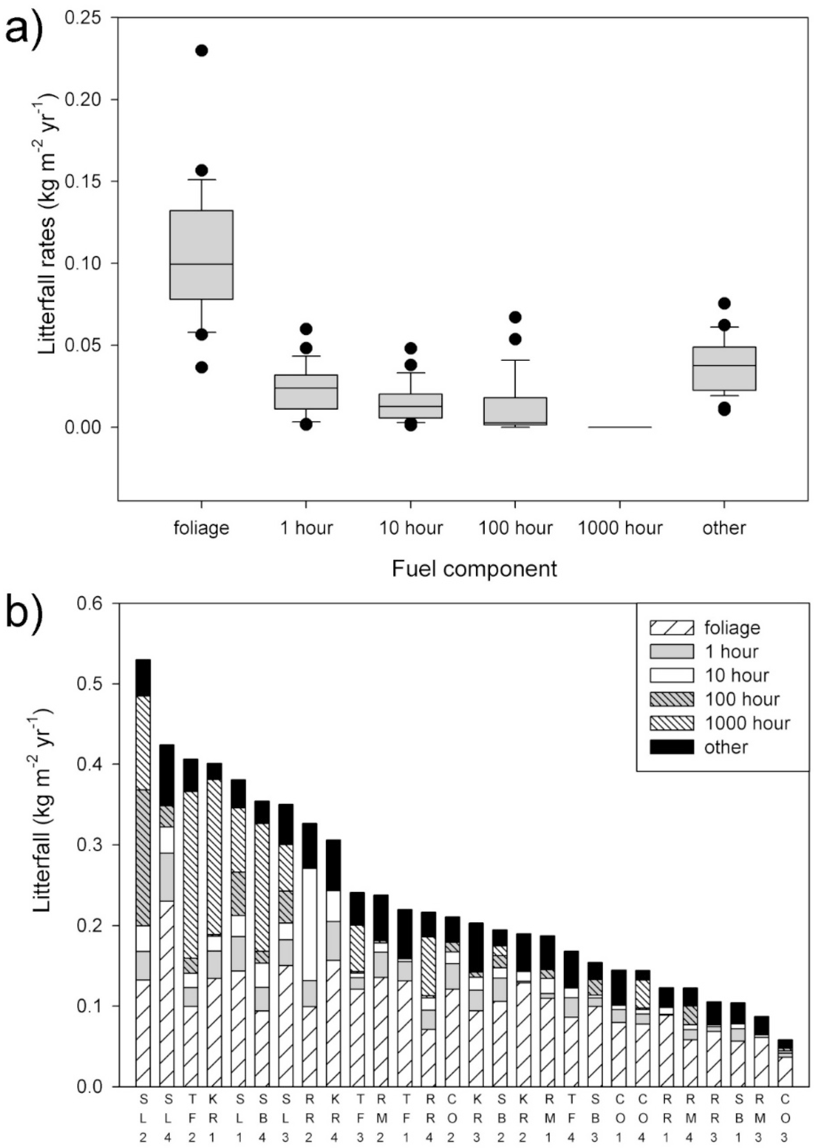
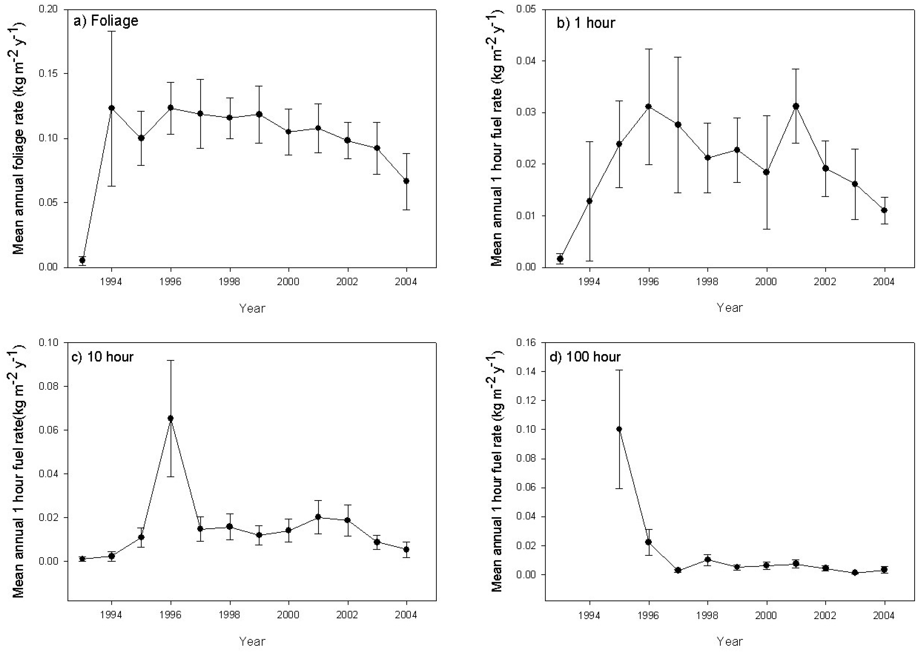
3.2.1. Deposition

In the FUELDYN study, Keane [31] found that rates of deposition (litterfall) varied by fuel component with foliage having the greatest deposition rates (0.05–0.15 kg·m−2·year−1) and the largest woody fuel components (100 and 1000 h) having the slowest rates (<0.03 kg·m−2·year−1) (Figure 5a). Moreover, fuel deposition varied greatly by site, from less than 0.05 kg·m−2·year−1 on unproductive sites (hot, dry and cold, wet) to ten times more (over 0.5 kg·m−2·year−1) on warm mesic sites (Figure 5b). These deposition rates were more closely correlated to vegetation characteristics than to environmental or climatic factors (e.g., temperature, elevation, and precipitation). In addition, deposition rates of each fuel component differed by site (Figure 5b); woody fuel deposition rates varied widely across all sites (an order of magnitude for 10, 100 h).
Keane [31] also found that the temporal pattern (i.e., annual variation) of deposited biomass differed by fuel component (Figure 6). It appeared that approximately the same amount of litter and 1 h woody fuels were deposited each year with little year-to-year variability, but the deposition of coarser woody fuels (10, 100 h) was more highly variable in time, with most coarse fuels deposited in one year (Figure 6). Keane [31] also found that only the foliage material was evenly deposited across the littertraps; all woody fuel components were unevenly distributed across both space and time.

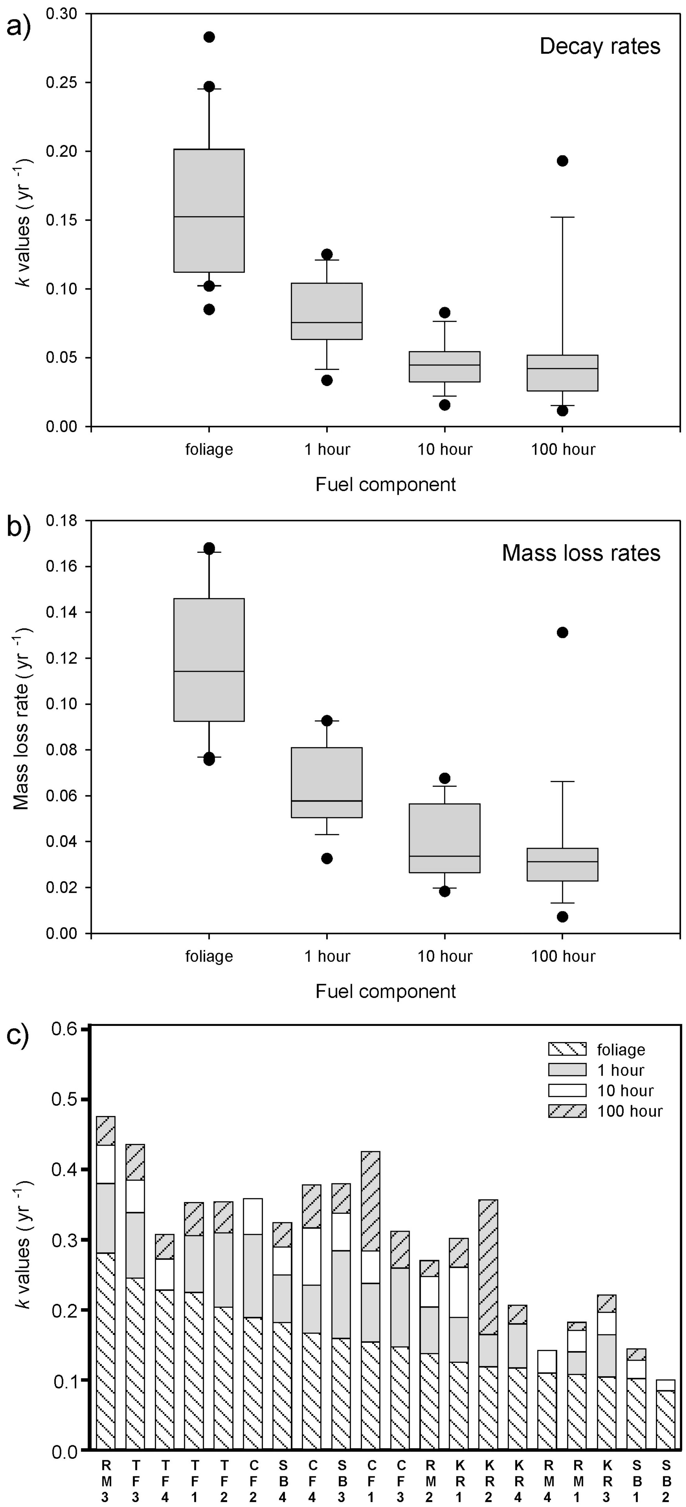
3.2.2. Decomposition

Similar to litterfall, decomposition also varies by fuel component and site (Figure 7). The smallest fuel particles (foliage) decayed at the fastest rates, often losing more than a fifth of their mass per year, while the coarser woody particles lost less than 5% of their weight each year (Figure 7a,d). Also, the rate of decomposition was greatly driven by an elevation gradient with the high elevation sites having the fastest decomposition (k values > 0.3 year−1) and the dry, hot low elevation sites had the slowest decomposition (k > 0.1 year−1). In fact, Keane [32] found decomposition rates were best correlated with climate gradients of temperature and moisture. To add to the complexity, measured decomposition rates for each fuel component also differed by site with rates of woody fuel decomposition often unrelated to foliar decomposition rates, and some larger woody fuels having k values greater than smaller woody fuels (Figure 7c).

4. Discussion

4.1. The Wildland Fuel Mosaic

Results from these two studies indicate that the landscape mosaic of wildland fuel is much more complex than we once thought [9]. Fuel components are distributed differently in space with fine fuels changing over spatial scales that are an order of magnitude smaller than coarse woody fuels and canopy fuels (Table 2). Fine fuel components are more uniformly distributed in space with lower variabilities than the high variability coarse fuels. The primary reasons for this complexity is that fuel components are deposited on the ground at different rates and patterns (Figure 4), and after they land on the ground, they decompose at different rates (Figure 7), and this deposition and decomposition are governed by different factors (vegetation controls deposition, climate controls decomposition). Fine fuels are added to the surface fuel layer at the greatest rates, but they may decompose quicker, whereas CWD particles are more scattered across space, and it may take decades to centuries for it to decompose depending on site factors.
A framework for understanding spatiotemporal surface and canopy fuel dynamics can be constructed from findings of these two studies [9,31]. First, the spatial locations of the plants that contribute both live and dead fuels provide the coarse template for spatial fuel dynamics. Existing plants grow and die, and new plants are always becoming established. The phenological, physiological, and morphological characteristics of the plants dictate the types of fuels (i.e., live and dead components) available for combustion. Dead material from these plants gets deposited on the ground in patterns based on particle size and weight, height of release, intercepting vegetation, and wind dynamics [25]; small particles may be blown great distances while large heavy particles tend to drop straight down. A greater amount of smaller particles, such as foliage and twigs, are deposited than the large particles, such as branches and logs (Figure 4). Once on the ground, the process of decay acts on these particles to further fracture and decompose organic components [37,38]. Rates of decomposition also depend on the size of the particle with smaller particles decomposing faster than large materials (Figure 6). So, while large particles are rarer than small particles, they have a longer residence time and they tend to be found near the parent plants [39]. Disturbance alters development and deposition rates by killing and maybe consuming whole plants and plant parts, and they can also change the pattern of surface dead fuel by consuming necromass and altering decomposition. The interactions of disturbance and decomposition processes with vegetation development and deposition controls wildland fuelbed properties thereby creating the dynamic fuel mosaic, and this changing fuel mosaic ultimately controls fire regimes.
Two factors that control fuel dynamics were not directly assessed in these two studies—vegetation development and disturbance. Rates of live fuel growth were not included in FUELDYN study because of time and cost considerations, and disturbance was ignored because FUELDYN sites were selected based on their lack of disturbance [31]. Had these two factors been studied, they probably would have revealed even greater complexity and corresponding variability in wildland fuel dynamics. In fact, the two sites in the FUELVAR study that were thinned had twice the variability in loading as the other sites. Live plant biomass accumulates at rates much greater than decompositional losses, and the diversity of species, sizes, and coverage of plants contributes to a diverse and complex set of canopy and surface fuel characteristics. And while biomass accumulation is slow and gradual, the effects of disturbance on wildland fuelbed dynamics may be immediate and extensive. Wildland fire, the most pervasive disturbance in the US northern Rocky Mountains [40,41], causes major changes in wildland fuelbeds through fuel consumption and fire-caused plant mortality. Disturbance impacts are also manifest differently by fuel component; most fine fuels are consumed in wildfires, for example, while the coarse fuels may only partially be consumed [42].

4.2. Implications

Findings from the FUELVAR and FUELDYN studies have sweeping implications for all of fire management. Traditional methods and sampling designs that are used to describe and inventory fuels may be fundamentally limited if they don’t recognize the high variability of fuel attributes across space and time [43]. Planar intersect sampling of woody fuel loadings, for example, may be inappropriate for describing spatial variability of woody fuel loading [44]. Conventional fuel inventory techniques, such as photo series [45], may be inappropriate because fuels vary at scales different from the scales represented by the picture in the series; the limited area of evaluation, for example, may be too small to accurately assess loadings for CWD [44]. Inappropriate sampling methods may result in higher uncertainty in fuel loadings that may mask subtle treatment effects [46]. Remotely sensed products used to map fuels, such as Landsat Thematic Mapper, may have resolutions that are inappropriate for capturing the spatial distribution of fuels, especially FWD [47]. Fuel classifications may be ineffective because fuel components vary independently of each other and the high variability of fuel characteristics within a site may overwhelm unique fuelbed identification across sites [43]. Keane et al. [48], for example, found that the high variability of fuel loadings within a classification category resulted in the inability of that category to be accurately mapped. Many fire hazard and risk analyses assume fuels do not change over time [49,50,51], yet temporal changes in surface and canopy fuels can be large enough to influence fire behavior predictions (Figure 7). High deposition rates, coupled with disturbance effects, may rapidly change fuelbed characteristics and quickly render fuel maps out-dated [47]. Each year, the US spends millions of dollars on fuel treatments that may fast become ineffective because the design failed to account for temporal fuel dynamics [52].
These findings also provide valuable insight into why it is so difficult to create accurate fuel applications and products for fire behavior modeling—complex ecological interactions create high spatiotemporal variability of fuel component characteristics that may compromise predictions. This variability is different for each fuel component and it is so high that it often overwhelms most statistical analyses and classification schemes [48]. Traditional approaches of over-simplifying fuel descriptions for fire simulations may rarely be appropriate, if they ever worked at all [9,46]. Fire behavior fuel models, for example, may provide acceptable results in a one-dimensional application, such as the BEHAVE model [53], but three-dimensional fire behavior models may need more realistic inputs of spatial fuel distributions [18].
Future wildland fuel applications and tools must account for high spatiotemporal variability to be effective in fire management. Instead of managing for average fuel conditions, the ranges and variations must be used to better approximate the highly variable stand conditions. Fire hazard and risk models must have the ability to simulate changes in the fuelbed due to the 4 D’s described above [54]. Fuel inventory and monitoring methods must have the ability to sample fuel components at their inherent spatial scale of distribution [44]. Fuel classifications must be designed to account for high variability in loading over multiple scales; Lutes et al. [55], for example, created a fuel classification of potential fire effects using field sampled fuel component loadings but failed to include measures of variability. Fuel maps must be designed to successfully link fuel component spatial scales with mapping methods, and these maps should be linked to fuel dynamics models to simulate potential changes that may render the map quickly outdated.

5. Summary

The ecological processes of vegetation development (succession), deposition, decomposition, and disturbance interact to create complex wildland fuel mosaics in the forests of the US northern Rocky Mountains. This fuel mosaic provides a template for future fire patterns, and its shifts over time influence the intrinsic fire regime that eventually emerges from the interactions of the fuel mosaic, fire ignition, and climate [41,56]. The fuel mosaic is constantly changing at rates dictated by the biophysical environment, the vegetation, and disturbance interactions. This dynamic character of fuel mosaics contributes to high spatiotemporal variability that confounds development and use of wildland fuel applications in fire management. Future wildland fuel applications must address both the spatial and temporal variability of wildland fuels to ensure accurate fuel inputs to fire management applications.

Acknowledgments

This work was partially funded by the USGS National Biological Service and Glacier National Park’s Global Change Research Program under Interagency Agreements 1430-1-9007 and 1430-3-9005 and the USGS CLIMET project. It was also funded using National Fire Plan Research monies.

Conflicts of Interest

The author declares no conflict of interest.

Abbreviations

The following abbreviations are used in this manuscript:
FUELVARA comprehensive project aimed at quantifying the spatial variability of fuels
FUELDYNA 12 years study quantifying litterfall and decomposition rates for US northern Rocky Mountain undisturbed stands
1 hdowned, dead woody fuel particles less than 6 mm in diameter
10 hdowned, dead woody fuel particles less than 25 mm in diameter
100 hdowned, dead woody fuel particles less than 76 mm in diameter
1000 hdowned, dead woody fuel particles greater than 76 mm in diameter
FWDall dead fuel particles below 76 mm in diameter
CWDall dead fuel particles greater than 76 mm in diameter

References

  1. Heyerdahl, E.K.; Brubaker, L.B.; Agee, J.K. Spatial controls of historical fire regimes: A multiscale example from the Interior West, USA. Ecology 2001, 82, 660–678. [Google Scholar] [CrossRef]
  2. Swetnam, T.W.; Betancourt, J.L. Fire-southern oscillation relations in the southwestern United States. Science 1990, 249, 1017–1020. [Google Scholar] [CrossRef] [PubMed]
  3. Weise, D.R.; Wright, C.S. Wildland fire emissions, carbon and climate: Characterizing wildland fuels. For. Ecol. Manag. 2014, 317, 26–40. [Google Scholar] [CrossRef]
  4. Rocca, M.E.; Brown, P.M.; MacDonald, L.H.; Carrico, C.M. Climate change impacts on fire regimes and key ecosystem services in Rocky Mountain forests. For. Ecol. Manag. 2014, 327, 290–305. [Google Scholar] [CrossRef]
  5. Agee, J.K.; Skinner, C.N. Basic principles of forest fuel reduction treatments. For. Ecol. Manag. 2005, 211, 83–96. [Google Scholar] [CrossRef]
  6. McKenzie, D.; Kennedy, M.C. Scaling laws and complexity in fire regimes. In The Landscape Ecology of Fire; McKenzie, D., Miller, C., Falk, D.A., Eds.; Springer Ltd.: Dordrecht, The Netherlands, 2011. [Google Scholar]
  7. McKenzie, D.; Shankar, U.; Keane, R.E.; Stavros, E.N.; Heilman, W.E.; Fox, D.G.; Riebau, A.C. Smoke consequences of new wildfire regimes driven by climate change. Earth’s Future 2014, 2, 35–59. [Google Scholar] [CrossRef]
  8. Reinhardt, E.D.; Keane, R.E.; Calkin, D.E.; Cohen, J.D. Objectives and considerations for wildland fuel treatment in forested ecosystems of the interior western United States. For. Ecol. Manag. 2008, 256, 1997–2006. [Google Scholar] [CrossRef]
  9. Keane, R.E. Wildland Fuel Fundamentals and Applications; Springer: New York, NY, USA, 2015. [Google Scholar]
  10. Harmon, M.E.; Franklin, J.F.; Swanson, F.J.; Sollins, P.; Gregory, S.V.; Lattin, J.D.; Anderson, N.H.; Cline, S.P.; Aumen, N.G.; Sedell, J.R.; et al. Ecology of coarse woody debris in temperate ecosystems. Adv. Ecol. Res. 1986, 15, 133–302. [Google Scholar]
  11. Keane, R.E.; Gray, K.; Bacciu, V. Spatial Variability of Wildland Fuel Characteristics in Northern Rocky Mountain Ecosystems; Research Paper RMRS-RP-98; USDA Forest Service Rocky Mountain Research Station: Fort Collins, CO, USA, 2012; p. 56.
  12. Kalabokidis, K.; Omi, P. Quadrat analysis of wildland fuel spatial variability. Int. J. Wildland Fire 1992, 2, 145–152. [Google Scholar] [CrossRef]
  13. Brown, J.K.; Bevins, C.D. Surface Fuel Loadings and Predicted Fire Behavior for Vegetation Types in the Northern Rocky Mountains; INT-358; U.S. Department of Agriculture, Forest Service, Intermountain Forest and Range Experiment Station: Ogden, UT, USA, 1986; p. 9.
  14. Waring, R.H.; Running, S.W. Forest Ecosystems: Analysis at Multiple Scales, 2nd ed.; Academic Press, Inc.: San Diego, CA, USA, 1998; p. 370. [Google Scholar]
  15. Menakis, J.P.; Keane, R.E.; Long, D.G. Mapping ecological attributes using an integrated vegetation classification system approach. J. Sustain. For. 2000, 11, 245–265. [Google Scholar] [CrossRef]
  16. Keane, R.; Gray, K.; Bacciu, V.; Leirfallom, S. Spatial scaling of wildland fuels for six forest and rangeland ecosystems of the northern Rocky Mountains, USA. Landsc. Ecol. 2012, 27, 1213–1234. [Google Scholar] [CrossRef]
  17. Stephens, S.L.; McIver, J.D.; Boerner, R.E.; Fettig, C.J.; Fontaine, J.B.; Hartsough, B.R.; Kennedy, P.L.; Schwilk, D.W. The effects of forest fuel-reduction treatments in the United States. BioScience 2012, 62, 549–560. [Google Scholar]
  18. Parsons, R.A.; Mell, W.E.; McCauley, P. Linking 3D spatial models of fuels and fire: Effects of spatial heterogeneity on fire behavior. Ecol. Model. 2010, 222, 679–691. [Google Scholar] [CrossRef]
  19. King, K.J.; Bradstock, R.A.; Cary, G.J.; Chapman, J.; Marsden-Smedley, J.B. The relative importance of fine-scale fuel mosaics on reducing fire risk in south-west Tasmania, Australia. Int. J. Wildland Fire 2008, 17, 421–430. [Google Scholar] [CrossRef]
  20. Reich, R.M.; Lundquist, J.E.; Bravo, V.A. Spatial models for estimating fuel loads in the Black Hills, South Dakota, USA. Int. J. Wildland Fire 2004, 13, 119–129. [Google Scholar] [CrossRef]
  21. Hiers, J.K.; O’Brien, J.J.; Mitchell, R.J.; Grego, J.M.; Loudermilk, E.L. The wildland fuel cell concept: An approach to characterize fine-scale variation in fuels and fire in frequently burned longleaf pine forests. Int. J. Wildland Fire 2009, 18, 315–325. [Google Scholar] [CrossRef]
  22. Peters, D.P.C.; Mariotto, I.; Havstad, K.M.; Murray, L.W. Spatial variation in remnant grasses after a grassland-to-shrubland state change: implications for restoration. Rangel. Ecol. Manag. 2006, 59, 343–350. [Google Scholar] [CrossRef]
  23. Theobald, D. A general model to quantify ecological integrity for landscape assessments and US application. Landsc. Ecol. 2013, 28, 1859–1874. [Google Scholar] [CrossRef]
  24. Kreye, J.K.; Varner, J.M.; Dugaw, C.J. Spatial and temporal variability of forest floor duff characteristics in long-unburned Pinus palustris forests. Can. J. For. Res. 2014, 44, 1477–1486. [Google Scholar] [CrossRef]
  25. Ferrari, J.B. Fine-scale patterns of leaf litterfall and nitrogen cycling in an old-growth forest. Can. J. For. Res. 1999, 29, 291–302. [Google Scholar] [CrossRef]
  26. Jin, S. Computer classification of four major components of surface fuel in Northeast China by image: The first step towards describing spatial heterogeneity of surface fuels by imags. For. Ecol. Manag. 2004, 203, 395–406. [Google Scholar] [CrossRef]
  27. Jia, G.J.; Burke, I.C.; Goetz, A.F.H.; Kaufmann, M.R.; Kindel, B.C. Assessing spatial patterns of forest fuels using AVIRIS data. Remote Sens. Environ. 2006, 102, 318–327. [Google Scholar] [CrossRef]
  28. Miller, C.; Urban, D.L. Connectivity of forest fuels and surface fire regimes. Landsc. Ecol. 2000, 15, 145–154. [Google Scholar] [CrossRef]
  29. Knapp, E.E.; Keeley, J.E. Heterogeneity in fire severity within early season and late season prescribed burns in a mixed-conifer forest. Int. J. Wildland Fire 2006, 15, 37–45. [Google Scholar] [CrossRef]
  30. Jenkins, M.J.; Page, W.G.; Hebertson, E.G.; Alexander, M.E. Fuels and fire behavior dynamics in bark beetle-attacked forests in Western North America and implications for fire management. For. Ecol. Manag. 2012, 275, 23–34. [Google Scholar] [CrossRef]
  31. Keane, R.E. Surface Fuel Litterfall and Decomposition in the Northern Rocky Mountains, USA; Research Paper RMRS-RP-70; USDA Forest Service Rocky Mountain Research Station: Fort Collins, CO, USA, 2008; p. 22.
  32. Keane, R.E. Biophysical controls on surface fuel litterfall and decomposition in the northern Rocky Mountains, USA. Can. J. For. Res. 2008, 38, 1431–1445. [Google Scholar] [CrossRef]
  33. Bellehumeur, C.; Legendre, P. Multiscale sources of variation in ecological variables: Modeling spatial dispersion, elaborating sampling designs. Landsc. Ecol. 1998, 13, 15–25. [Google Scholar] [CrossRef]
  34. Townsend, D.E.; Fuhlendorf, S.D. Evaluating Relationships between Spatial Heterogeneity and the Biotic and Abiotic Environments. Am. Midl. Nat. 2010, 163, 351–365. [Google Scholar] [CrossRef]
  35. Fortin, M.-J. Spatial statistics in landscape ecology. In Landscape Ecological Analysis: Issues and Applications; Klopatek, J.M., Gardner, R.H., Eds.; Springer-Verlag, Inc.: New York, NY, USA, 1999; pp. 253–279. [Google Scholar]
  36. Olson, J. Energy storage and the balance of the producers and decomposers in ecological systems. Ecology 1963, 44, 322–331. [Google Scholar] [CrossRef]
  37. Harmon, M.E.; Krankina, O.N.; Sexton, J. Decomposition vectors: A new approach to estimating woody detritus decomposition dynamics. Can. J. For. Res. 2000, 30, 76–84. [Google Scholar] [CrossRef]
  38. Kaarik, A.A. Decomposition of wood. In Biology of Plant Litter Decomposition; Dickinson, C.H., Pugh, G.J.F., Eds.; Academic Press: London, UK, 1974; Volume 1, pp. 129–174. [Google Scholar]
  39. Harmon, M.E.; Hua, C. Coarse woody debris dynamics in two old-growth ecosystems. Bioscience 1991, 41, 604–610. [Google Scholar] [CrossRef]
  40. McKenzie, D.; Miller, C.; Falk, D.A. The Landscape Ecology of Fire; Springer Ltd.: Dordrecht, The Netherlands, 2011. [Google Scholar]
  41. Scott, A.C.; Bowman, D.M.J.S.; Bond, W.J.; Pyne, S.J.; Alexander, M.E. Fire on Earth: An Introduction; John Wiley and Sons Ltd.: Chichester, UK, 2014; p. 413. [Google Scholar]
  42. Brown, J.K.; Reinhardt, E.D.; Fischer, W.C. Predicting duff and woody fuel consumption in northern Idaho prescribed fires. For. Sci. 1991, 37, 1550–1566. [Google Scholar]
  43. Keane, R.E. Describing wildland surface fuel loading for fire management: A review of approaches, methods and systems. Int. J. Wildland Fire 2013, 22, 51–62. [Google Scholar] [CrossRef]
  44. Keane, R.E.; Gray, K. Comparing three sampling techniques for estimating fine woody down dead biomass. Int. J. Wildland Fire 2013, 22, 1093–1107. [Google Scholar] [CrossRef]
  45. Fischer, W.C. Photo Guide for Appraising Downed Woody Fuels in Montana Forests: Interior Ponderosa Pine, Ponderosa Pine-Larch-Douglas-Fir, Larch-Douglas-Fir, and Interior Douglas-Fir Cover Types; INT-97; USDA Forest Service Intermountain Research Station: Ogden, UT, USA, 1981; p. 133.
  46. Sikkink, P.G.; Keane, R.E. A comparison of five sampling techniques to estimate surface fuel loading in montane forests. Int. J. Wildland Fire 2008, 17, 363–379. [Google Scholar] [CrossRef]
  47. Keane, R.E.; Burgan, R.E.; Wagtendonk, J.V. Mapping wildland fuels for fire management across multiple scales: Integrating remote sensing, GIS, and biophysical modeling. Int. J. Wildland Fire 2001, 10, 301–319. [Google Scholar] [CrossRef]
  48. Keane, R.E.; Herynk, J.M.; Toney, C.; Urbanski, S.P.; Lutes, D.C.; Ottmar, R.D. Evaluating the performance and mapping of three fuel classification systems using Forest Inventory and Analysis surface fuel measurements. For. Ecol. Manag. 2013, 305, 248–263. [Google Scholar] [CrossRef]
  49. Hall, S.A.; Burke, I.C. Considerations for characterizing fuels as inputs for fire behavior models. For. Ecol. Manag. 2006, 227, 102–114. [Google Scholar] [CrossRef]
  50. Finney, M.A. Design of regular landscape fuel treatment patterns for modifying fire growth and behavior. For. Sci. 2001, 47, 219–228. [Google Scholar]
  51. Finney, M.A. A Computational Method for Optimizing Fuel Treatment Locations. In Fuels management-how to measure success, Proceedings of the Rocky Mountain Research Station Conference; Portland, OR, USA, 28–30 March 2006, Andrews, P.L., Butler, B.W., Eds.; U.S. Department of Agriculture, Forest Service, RMRS-P-41: Portland, OR, USA, 2006; pp. 107–123. [Google Scholar]
  52. Parks, S.A.; Miller, C.; Holsinger, L.M.; Baggett, L.S.; Bird, B.J. Wildland fire limits subsequent fire occurrence. Int. J. Wildland Fire 2016, 25, 182–190. [Google Scholar] [CrossRef]
  53. Andrews, P.L. BehavePlus Fire Modeling System, Version 4.0: Variables; RMRS-GTR-213WWW; USDA Forest Service Rocky Mountain Research Station: Fort Collins, CO, USA, 2008; p. 107.
  54. Beukema, S.J.; Greenough, J.A.; Robinson, D.C.E.; Kurtz, W.A.; Reinhardt, E.D.; Crookston, N.L.; Brown, J.K.; Hardy, C.C.; Stage, A.R. An introduction to the Fire and Fuels Extension to FVS. In Proceedings of the Forest Vegetation Simulator Conference; Ft. Collins, CO, USA, 3–7 February 1997, Teck, R., Moeur, M., Adams, J., Eds.; United States Department of Agriculture, Forest Service, Intermountain Forest and Range Experiment Station: Ft. Collins, CO, USA, 1997; pp. 191–195. [Google Scholar]
  55. Lutes, D.C.; Keane, R.E.; Caratti, J.F. A surface fuels classification for estimating fire effects. Int. J. Wildland Fire 2009, 18, 802–814. [Google Scholar] [CrossRef]
  56. Bowman, D.M.J.S.; Balch, J.K.; Artaxo, P.; Bond, W.J.; Carlson, J.M.; Cochrane, M.A.; D’Antonio, C.M.; DeFries, R.S.; Doyle, J.C.; Harrison, S.P.; et al. Fire in the Earth System. Science 2009, 324, 481–484. [Google Scholar] [CrossRef] [PubMed]
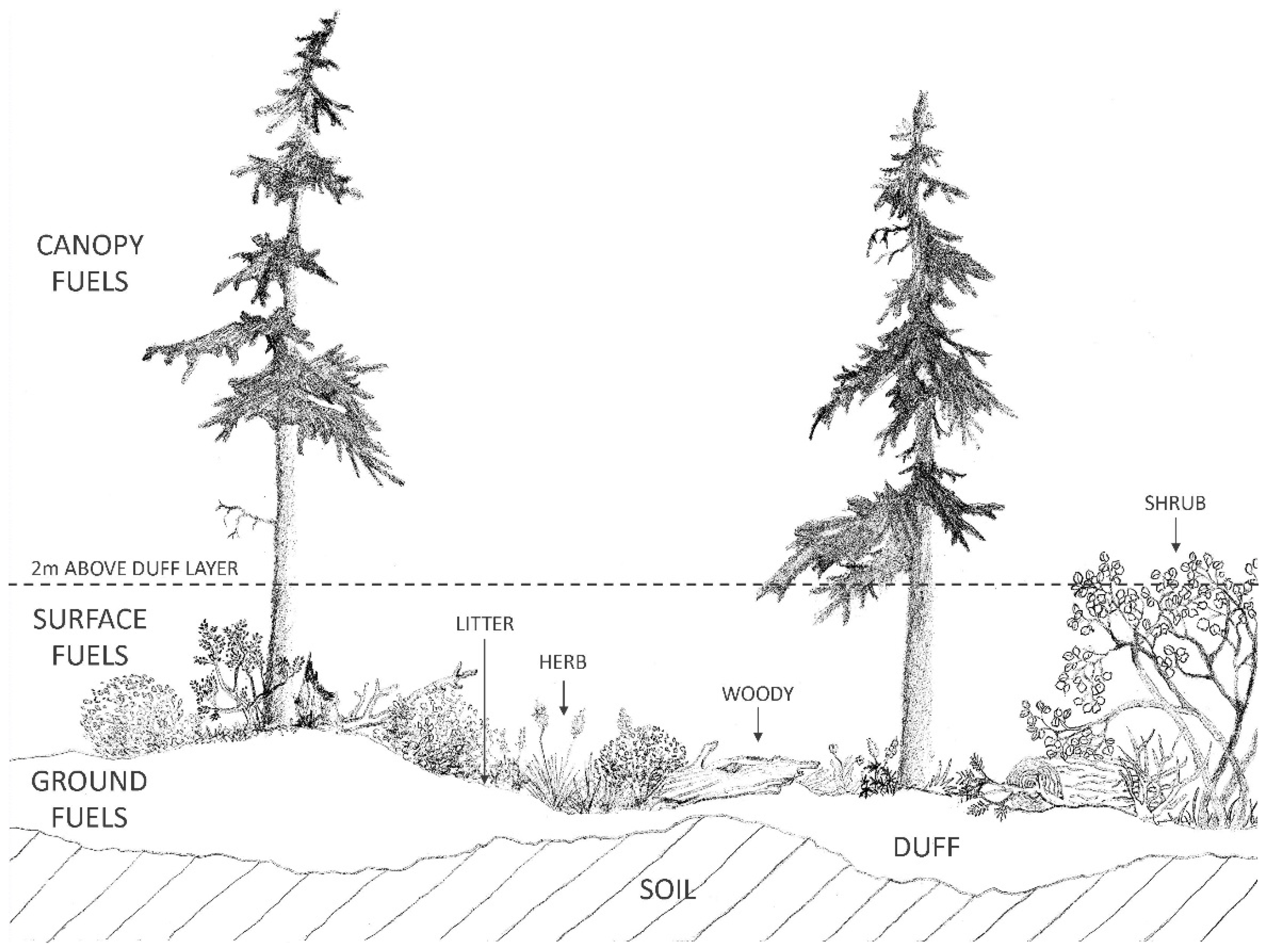
Figure 1. Illustration of a wildland forest fuelbed showing the three major strata: ground, surface, and canopy fuels from Keane [9] and drawn by Ben Wilson.
Forests 07 00129 g001
Figure 2. The sampling design of the FUELVAR study showing (a) the 1 km2 sampling grid, (b) the intensification of the grid, and (c) the nested plot sampling scheme in the upper right.
Forests 07 00129 g002
Figure 3. The sampling design of the FUELDYN study showing the (a) seven sampling sites; (b) the four plots per sampling site placed at high and low elevations and north and south aspects; (c) the littertrap placement within the 400 m2 plot; and (d) the decomposition bag placement on the 400 m2 plot.
Forests 07 00129 g003
Figure 4. Relationship of semi-variogram range (m) with the size of fuel particle represented by diameter (cm).
Forests 07 00129 g004
Figure 5. The amount of fuel deposited each year (litterfall) by (a) fuel component and (b) the 28 sites in the Keane [31] study. Site descriptions ID numbers on the X axis can be found in Keane [31]. Sites are arranged in order of productivity from highest to lowest.
Forests 07 00129 g005
Figure 6. Coarser fuels have higher interannual variability. The amount of deposited biomass by fuel component on the Coram site over 12 years of collection (a) foliage (litter); (b) 1 h; (c) 10 h; and (d) 100 h.
Forests 07 00129 g006
Figure 7. Rates of decomposition expressed as (a) k values for each fuel component, (b) mass loss rates for each fuel component; and (c) k values for each site by fuel component. Site descriptions ID numbers on the X axis can be found in Keane [31]. Sites are arranged in order of elevation from highest to lowest. Some sites did not have decomposition estimates [31].
Forests 07 00129 g007
Table 1. Descriptions of the three canopy fuel characteristics, eight surface fuel components, and one ground fuel components included in this paper. FWD is fine woody debris, a term often given to wood fuel particles less than 8 cm in diameter. CWD is coarse woody debris, a term used to woody fuel particles greater than 8 cm in diameter. Those fuel components in bold indicate that they were included in the FUELDYN project, while all fuel components were included in the FUELVAR project.
Fuel TypeFuel Component/AttributeCommon NameSizeDescription
Canopy Fuels
CanopyCanopy bulk density (kg·m−3)CBD<3 mm diameterAll canopy material less than 3 mm diameter
Canopy fuel loading (kg·m−2)CFL<3 mm diameterAll canopy material less than 3 mm diameter
Canopy cover (%)CCAll materialVertically projected canopy cover
Surface Fuels
Downed Dead Woody1 h woodyTwigs, FWD<0.6 cm (0.25 inch) diameterDetached woody fuel particles on the ground
10 h woodyBranches, FWD0.6–2.5 cm (0.25–1.0 inch) diameterDetached woody fuel particles on the ground
100 h woodyLarge Branches, FWD2.5–8 cm (1–3 inch) diameterDetached woody fuel particles on the ground
1000 h woodyLogs, CWD8+ cm (3+ inch) diameterDetached woody fuel particles on the ground
ShrubsShrubShrubbyAll shrubby material less than 5 cm diameterAll burnable shrubby biomass with branch diameters less than 5 cm
HerbaceousHerbHerbsAll sizesAll live and dead grass, forb, and fern biomass
LitterLitterLitterAll sizes, excluding woodyFreshly fallen non-woody material which includes leaves, cones, pollen cones
Ground Fuels
DuffDuffDuffAll sizesPartially decomposed biomass whose origins cannot be determined
Table 2. Semi-variogram range statistics for all surface fuel components and three canopy fuel variables across the six FUELVAR sites. Empty cells indicate no spatial model could be fit to the data. Canopy fuel attributes: CBD-Canopy bulk density, CFL-Canopy fuel load, and CC-Canopy cover.
Fuel ComponentSagebrush GrasslandPinyon JuniperPonderosa Pine SavannaPonderosa Pine-FirPine- Fir-LarchLodgepole Pine
Range (m)
1 h4.72.52.816.38.96.0
10 h6.62.40.94.92.211.1
100 hNo 100 h2.52.54.62.44.1
1000 hNo LogsNo Logs84.022.087.3157.0
Shrub2.415.10.91.83.62.7
Herb0.71.10.83.50.51.8
Litter + Duff0.51.42.51.30.50.9
CBDNo trees440.0-412.0100.0120.0
CFLNo trees560.0-600.0310.0560.0
CCNo trees407.0--230.0300.0

