Article

Tree Mortality Undercuts Ability of Tree-Planting Programs to Provide Benefits: Results of a Three-City Study

1
School of Public and Environmental Affairs, Indiana University, Bloomington, IN 47405, USA
2
Bloomington Urban Forestry Research Group, Indiana University, Bloomington, IN 47408, USA
3
The Vincent and Elinor Ostrom Workshop in Political Theory and Policy Analysis, Indiana University, Bloomington, IN 47408, USA
4
Department of Environmental Science and Studies, College of Science and Health, DePaul University, Chicago, IL 60614, USA
*
Author to whom correspondence should be addressed.
Forests 2016, 7(3), 65; https://doi.org/10.3390/f7030065
Submission received: 16 December 2015 / Revised: 4 March 2016 / Accepted: 9 March 2016 / Published: 11 March 2016
(This article belongs to the Special Issue Urban and Periurban Forest Diversity and Ecosystem Services)

Abstract

:
Trees provide numerous benefits for urban residents, including reduced energy usage, improved air quality, stormwater management, carbon sequestration, and increased property values. Quantifying these benefits can help justify the costs of planting trees. In this paper, we use i-Tree Streets to quantify the benefits of street trees planted by nonprofits in three U.S. cities (Detroit, Michigan; Indianapolis, Indiana, and Philadelphia, Pennsylvania) from 2009 to 2011. We also use both measured and modeled survival and growth rates to “grow” the tree populations 5 and 10 years into the future to project the future benefits of the trees under different survival and growth scenarios. The 4059 re-inventoried trees (2864 of which are living) currently provide almost $40,000 (USD) in estimated annual benefits ($9–$20/tree depending on the city), the majority (75%) of which are increased property values. The trees can be expected to provide increasing annual benefits during the 10 years after planting if the annual survival rate is higher than the 93% annual survival measured during the establishment period. However, our projections show that with continued 93% or lower annual survival, the increase in annual benefits from tree growth will not be able to make up for the loss of benefits as trees die. This means that estimated total annual benefits from a cohort of planted trees will decrease between the 5-year projection and the 10-year projection. The results of this study indicate that without early intervention to ensure survival of planted street trees, tree mortality may be significantly undercutting the ability of tree-planting programs to provide benefits to neighborhood residents.

1. Introduction

1.1. Benefits of Urban Trees

The urban forest provides many benefits (i.e., ecosystem services) for urban residents, from stormwater mitigation and air pollutant removal to reduced crime rates and better psychological well-being [1,2,3,4,5,6,7]. Nonprofit organizations and municipalities plant substantial numbers of young trees, sometimes in large tree-planting or canopy campaigns, to increase the provisioning of these benefits for urban residents (e.g., Philly Plant One Million Campaign (in Philadelphia, Pennsylvania), MillionTreesNYC (in New York City, New York), Mile High Million (in Denver, Colorado), etc.). These entities incur significant costs to plant and maintain trees [8,9], yet there is often little post-planting monitoring to assess whether the trees survive after planting. Additionally, the benefits of the trees are often presumed rather than measured or quantified.

1.2. Value of Quantifying Benefits

Quantification of the benefits provided by the urban forest can be used to help justify the costs of planting and maintaining trees and encourage investment in green infrastructure, and is also useful for evaluating goals associated with tree planting. For example, tree-planting campaigns are often undertaken to reduce combined sewer overflows or sequester carbon and reduce energy usage to mitigate the effects of climate change (e.g., Plant One Million 2015, City Plants 2015). Estimation of the amount (or monetary value) of stormwater intercepted or carbon sequestered by the planted trees could be used to evaluate whether the tree-planting programs are meeting their goals in a cost-effective manner. Assigning a monetary value to tree benefits also allows people to better understand the value of trees.
However, trees do not provide as many benefits when they are young and small as they do when they are large, mature, and healthy (Figure 1). Therefore, an estimation of benefits at the time the trees are planted will significantly undervalue the benefits the trees will provide in the future. An accurate prediction of the benefits trees will provide when they are mature would be more useful, for example, when conducting a cost-benefit analysis of a tree-planting program. Yet there are few to no programs that allow the user to employ locally relevant, empirically generated growth and survival rates to estimate the future benefits of planted trees.

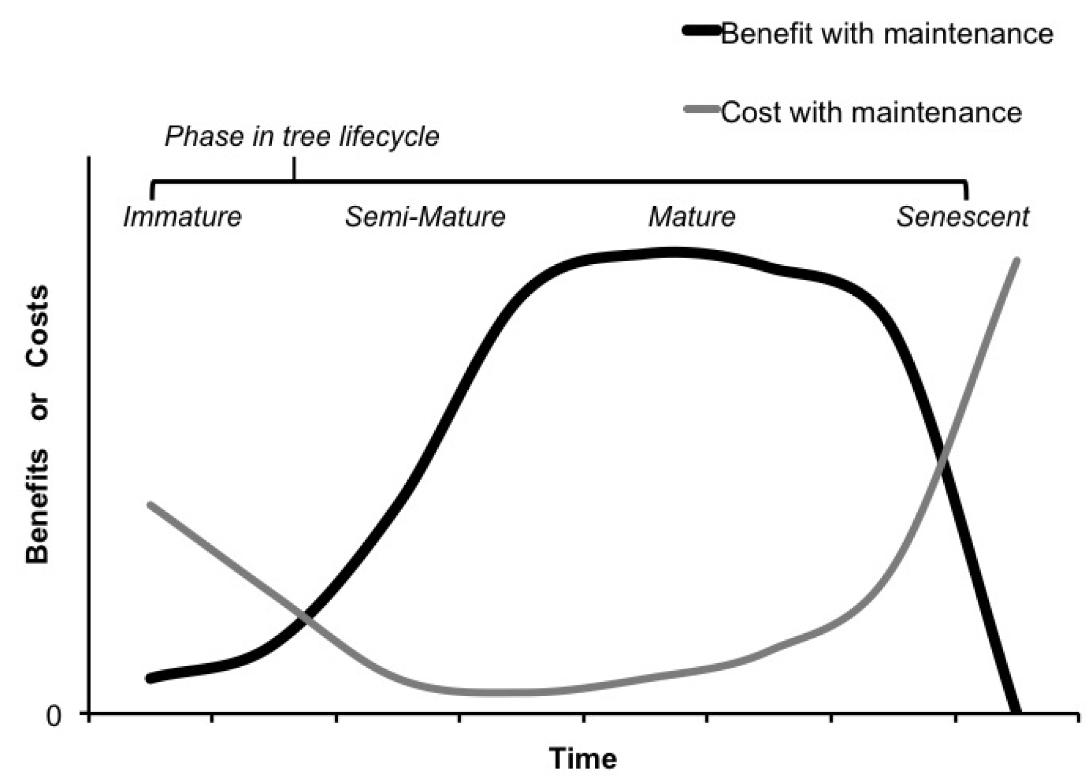
1.3. Costs Associated with Trees

Street trees provide benefits to urban residents, but there are also costs associated with these trees. In general, the costs of trees are not as well quantified or monetized as the benefits of trees [10]. A recent review of the cost of maintaining the urban forest categorizes the costs of trees as direct costs of planting and maintaining trees, costs of repairs to infrastructure damaged by street trees, costs of negative externalities associated with trees (i.e., ecosystem disservices), and opportunity costs [10], but others include infrastructure damage as an ecosystem disservice (e.g., [11,12]). Direct costs include all of the costs associated with planting and maintaining trees, including the purchase of the tree, cost of planting the tree, and subsequent pruning, watering, leaf removal, program administration, and eventual tree and stump removal/disposal [8,9,10]. Typical infrastructure interference costs are the costs of pavement and sewer repair and power outages caused by falling limbs or trees [10,13,14]. Some important negative externalities, or ecosystem disservices, associated with trees include emissions of biogenic VOCs, release of carbon dioxide (CO2) during maintenance activities and from leaf and wood decomposition, and allergies caused by pollen release [10,12]. Finally, opportunity costs include the lost space that could have been dedicated to parking, bike lanes, sidewalk cafes, or other uses of the public right-of-way, and the lost money that could have been spent on another program [10].
In a true cost-benefit analysis (CBA), where the object is to obtain the net benefits of a project or program (e.g., a project to plant a certain number of trees), all of the above costs must be monetized and weighed against all of the benefits that trees provide. We acknowledge the utility of conducting CBAs: (1) to determine whether the net benefits derived, in strictly numeric, monetary terms, justify the investment; or (2) to compare and select the socially optimal investment strategy among a set of options (i.e., select the program with the highest net benefits, or select the highest benefit-to-cost ratio) [15]. However, the aim of this study is not to conduct a CBA, but to analyze how the total (not net) benefits (as calculated by the i-Tree Streets software) change as the trees grow during the decade or so after transplanting and estimate how the benefits are affected by different growth and survival scenarios.

1.4. i-Tree Streets

To facilitate quantification and monetization of urban tree benefits, the U.S. Forest Service, Davey Resource Group, and other organizations partnered to produce i-Tree, a suite of programs that can be used to estimate the benefits provided by the urban forest [16,17]. This paper will focus on the use of i-Tree Streets (Version 5.1.5), which is designed to estimate the monetary value of the benefits of public and private street trees based on inventory data. We use i-Tree Streets to estimate the current benefits provided by recently planted trees in three U.S. cities. In addition, we use growth and survival rates measured for each study city to project the samples of trees 5 and 10 years into the future and estimate the annual benefits of the resulting populations in i-Tree Streets. We also model different survival and growth rates to elucidate the effects of increased survival and faster growth on the estimated benefits of the subsequent population. We acknowledge that the benefit estimates we report are used for comparison, as a translation of tree population characteristics (including growth and survival rates) into monetary values (in US Dollars) as outputs from i-Tree, and may not reflect actual benefits as valued and experienced by community residents. Based on this study, we conclude that survival is more important than growth in determining future benefits derived from a population of street trees.

2. Materials and Methods

2.1. Study Sites

The Bloomington Urban Forestry Research Group (BUFRG) at Indiana University (Bloomington, Indiana, USA [18]) was funded by the U.S. Forest Service’s National Urban and Community Forestry Advisory Council (NUCFAC) to conduct a study of tree planting projects supported by nonprofit organizations in urban settings in five U.S. cities [19]. The overall goal of the project was to evaluate the outcomes of neighborhood tree-planting programs. We partnered with the Alliance for Community Trees (ACTrees) and five of its nonprofit member organizations, Trees Atlanta, The Greening of Detroit, Keep Indianapolis Beautiful, Inc., the Pennsylvania Horticultural Society, and Forest ReLeaf of Missouri, to conduct this research. The study included a re-inventory (conducted during the summer of 2014) of trees planted in projects funded by these nonprofits from 2009 to 2011. This paper will focus on the cities that had large numbers (>1000) of trees re-inventoried during 2014: Detroit, Michigan; Indianapolis, Indiana; and Philadelphia, Pennsylvania.

2.2. Planted Tree Re-Inventory

Teams of citizen scientists (volunteers and/or high school and college students) trained by BUFRG researchers conducted a planted tree re-inventory [20,21] in summer 2014. The trees in the sample were planted through neighborhood tree-planting projects funded by our nonprofit partners in 2009, 2010, or 2011. All re-inventoried trees were street trees planted in the public right-of-way or very near the public right-of-way (i.e., an adjacent front yard). Trees were re-inventoried in 25 randomly selected neighborhoods per city. For the purposes of this research, a “neighborhood” was defined as a census block group. We randomly selected 25 block groups from the list of all block groups in the city that contained one or more trees planted as part of a planting project of greater than 20 trees.
The re-inventory protocol includes a suite of variables and methods to collect information on the tree, the surrounding growing environment, and evidence of care and maintenance (see [20,21] for complete variable list). The relevant variables for the present study were tree species, caliper (diameter at 6 in (15 cm) above the base of the tree), diameter at breast height (DBH; taken 4.5 ft (1.37 m) up the trunk of the tree), and overall condition rating. The overall condition ratings assigned to trees were good, fair, poor, dead, sprouts, stump, shrub, or absent (see Table 1 for overall condition rating definitions). Condition ratings were not used directly to calculate tree benefits in i-Tree, but were used to calculate survival rates and identify trees that were more likely to die and remove these trees from the population first in benefits projections (see Section 2.8 and Section 2.10 below). We had locations and species of every tree planted between 2009 and 2011 by the partner nonprofit in each of the cities, which facilitated the re-inventory and enabled data collectors to assign the condition rating of “absent” if the tree was missing or had been replaced with a different species. Within each randomly selected neighborhood, we assessed survival status for all trees and collected the suite of re-inventory variables for at least every other tree in the neighborhood as time allowed.
In addition to locations and species of trees, our nonprofit partners also provided us with an approximation of the caliper-at-planting and exact date (e.g., 30 October 2009) or season (e.g., Fall 2009) the tree was planted. We merged these data with the re-inventory data in Stata [22] to obtain a complete data set with planting and re-inventory variables for each re-inventoried tree.

2.3. How i-Tree Works

i-Tree Streets (Version 5.1.5) estimates the monetary value of benefits in five categories: energy, carbon, air quality, stormwater, and property value benefits. The benefit estimates are influenced by: (1) the size (diameter at breast height, or DBH) and species of the trees; (2) the annual rainfall and number of heating and cooling days for the climate zone; and (3) the prices assigned to benefits, including the cost of stormwater management, the cost of energy for heating and cooling, and the average home resale value. Crown size, leaf area, and growth of common street tree species in each climate zone are based on data collected in the reference city for each climate zone, published in the i-Tree regional community tree guides (Table 2). The climate zones relevant to this study were the Lower Midwest, which includes Indianapolis, and the Northeast, which includes Detroit and Philadelphia [8,9]. The Northeast climate zone is characterized as having more rainfall and more air pollution than the Lower Midwest, meaning that air quality and stormwater benefits are expected to be relatively more important in the Northeast than in the Lower Midwest. Growth of trees is also modeled differently in the two climate zones, as i-Tree models growth using logistic equations in the Lower Midwest and uses linear and logistic equations in the Northeast [8,9]. The difference in growth models affects the annual benefit estimates particularly for large (>30 cm DBH) trees (see Discussion Section 4.2 for more details).
i-Tree models tree species that were not measured in the reference city as a similar species and uses the midpoint of each size class interval to represent all the trees in that size class. Most benefit types are calculated based on estimated annual leaf area increase [8]. Annual leaf area increases and other aspects of tree structure are estimated from the measured DBHs based on predictive equations [23,24]. The monetary value of benefits per leaf area for each benefit type is determined by empirical data collected by U.S. Forest Service researchers in various US cities [1,25,26] and adjusted based on local prices (set by the user).

2.4. Preparation for i-Tree

Some transformations were required to prepare re-inventory data for i-Tree. First, all dead, sprout, stump, shrub, or absent trees, trees with no DBH recorded, and trees with no species recorded were removed from the data set. A new data set was created with only the species name, DBH, and overall condition rating for each remaining entry. Tree species names were replaced with the corresponding i-Tree species codes (originally developed by the U.S. Department of Agriculture for all plants; http://plants.usda.gov). If i-Tree did not have a species code for a certain tree species, that tree was assigned the species code of a closely related species (i.e., a species in the same genus) or assigned a general designation such as other broadleaf deciduous medium (BDM OTHER). For some genera, such as Malus and Lagerstroemia, i-Tree does not have species designations, and every tree in that genus is listed as, for example, Malus sp. This simplification avoids the complication of genera that have many cultivars that are genetic hybrids or crosses of multiple species.

2.5. Generating Benefit Estimates in i-Tree Streets

Because of the nature of our data (street tree inventory data), we chose to use i-Tree Streets, which uses species and diameter at breast height (DBH) of trees to estimate the benefits they provide. For each city, we set the climate zone, which determines the temperature and precipitation models used (see Table 2 for climate zone used for each study city). i-Tree allows the user to indicate whether the inventory type is “complete” or a sample, and we used the “complete” option to get an estimate of benefits only for the sampled trees. We did not modify the default prices for costs associated with trees, but we did customize the benefit prices for each city. The home prices were obtained from Trulia.com (Detroit and Philadelphia) and Zillow.com (Indianapolis). Electricity and natural gas prices were obtained from DTE Energy [27] (Detroit), Citizens Energy Group [28] (Indianapolis), and the Pennsylvania Public Utility Commission [29] (Philadelphia).
For each city, we defined size classes as 0–5 cm, 5–10 cm, 10–15 cm, 15–20 cm, 20–25 cm, 25–30 cm, and 30–1000 cm (i-Tree does not allow the user to change the upper limit of the largest size class). Trees with a DBH of exactly the breakpoint between size classes are included in the larger size class (i.e., a 5 cm tree will be included in the 5–10 cm size class).
Once all the parameters were set for the city, we imported the inventory data. For each city, we generated “All Benefits-Costs Reports” and a “Population Summary” report. These reports were exported from i-Tree and saved with metadata to keep track of the parameters used. We considered the main outcomes to be the total annual benefit estimates and the amount of annual benefit estimates of each type, both reported in monetary terms as US Dollar values.

2.6. Estimating Costs

Although we do not conduct an explicit cost-benefit analysis in this study (see Section 1.3 above), we do compare i-Tree-calculated benefits to two different estimates of the costs associated with the trees in this study. Average annual per-tree costs are obtained from the i-Tree community tree guides [8,9]. These cost estimates include planting, pruning, removal/disposal, infrastructure damage, irrigation, cleanup, liability/legal, and administrative costs. The total expected costs for a tree that lives 40 years are averaged over that 40-year period, so the estimated annual costs are assumed to be constant [8,9]. (Note that this assumption is very different from the actual likely distribution of costs over the lifetime of a tree as schematized in Figure 1 above.) We also present estimates of the initial planting and watering costs (i.e., establishment costs—the major monetary costs associated with young, small trees) obtained from one of our nonprofit partners to provide a more relevant cost to benefit comparison for the recently planted trees in Indianapolis.
Ecosystem disservices are not explicitly accounted for in either of our cost estimates; however, i-Tree subtracts biogenic VOC emissions from the total air quality benefits and subtracts CO2 released through maintenance activities and decomposition from the total carbon benefits [8,9], so those costs are factored into the benefit estimates we present.

2.7. Calculating Cumulative Benefits

Since we assumed linear growth rates (a constant increase in diameter per year) for 5- and 10-year projections, we can use the midpoint of each 5-year time period multiplied by 5 years to calculate cumulative benefits accrued over the time period (see Table 3). The cumulative benefits accrued during the first time period between planting and re-inventory (2014) were estimated as half the annual benefits at the time of re-inventory multiplied by 4 years, since the trees were between 3 and 5 years old at re-inventory. Cumulative benefits for the 5-year projection (2019; 8–10 years after planting) are calculated as the cumulative benefits at re-inventory, plus the annual benefits at year 2017 multiplied by 5 years. Cumulative benefits for the 10-year projection (2024; 13–15 years after planting) are calculated as the cumulative benefits for the 5-year projection (2019), plus the annual benefits at year 2022 multiplied by 5 years.

2.8. Calculating Annual Survival Rates

We calculated growth and survival rates of the recently planted trees separately for each city. The survival rate was based on the condition rating assigned to the tree: good, fair, or poor trees were rated as alive and absent, dead, shrub, stump, or sprout trees were rated as dead. To account for the fact that not all trees were the same age, we calculated an annual survival rate, Iannual, defined as
I a n n u a l = I t t
where t is the number of years since planting and It is the cumulative survival rate for all trees planted in a given year [30]. We used half years to designate the difference between fall and spring plantings. For simplicity we are assuming that trees were planted at the beginning of their indicated planting season and were re-inventoried more than halfway through the summer (Though we had exact planting dates for two of the three study cities, we used a seasonal grouping for all cities in this project for consistency across cities.), so t = 3.5 years since planting for trees planted in Spring 2011, and t = 3 years since planting for trees planted in Fall 2011. We calculated the annual survival rate separately for trees planted in Spring 2009, Fall 2009, Spring 2010, Fall 2010, Spring 2011, and Fall 2011, and used an average weighted by the number of trees planted each season to represent the overall annual survival rate for the city.

2.9. Calculating Growth Rates

We calculated growth of trees as relative growth rate, defined as
r e l a t i v e   g r o w t h   r a t e = ln   C 2 ln   C 1 N u m b e r   o f   g r o w i n g   s e a s o n s   s i n c e   p l a n t i n g
where C1 and C2 are measurements of tree caliper at the time of planting and time of re-inventory, respectively (after [31] as adapted by [32]). The 2014 growing season was counted towards growth, so the oldest trees (those planted in Spring 2009) had 6 growing seasons since planting and the youngest trees (those planted in Fall 2011) had 3.

2.10. Projecting Future Mortality

In each city, we modeled survival of the re-inventoried trees 5 and 10 years into the future with three different scenarios: one in which the annual survival rate was the same as that found for the first 3–6 seasons of growth (establishment-phase survival rate), one in which the annual survival rate was 96.4%, corresponding to annual survival found in the literature review by Roman and Scatena [30], and one in which no trees died after 2014 (the no additional mortality scenario). The “no additional mortality” scenario is not realistic, but it represents how the population will look if all of the currently living trees survive for the next 5 or 10 year period. It is likely that the survival rate will increase after the trees are established because annual mortality is highest during the establishment phase [33,34,35]; hence we modeled scenarios in which survival rates were higher than in the establishment phase. We also predicted that trees that were in poor condition at the time of re-inventory were more likely to die, so those trees were eliminated from the dataset first in modeled mortality. Within condition rating, trees were eliminated randomly (i.e., not by size or species).
To randomize mortality, we used Stata [22] to assign a random number between 0 and 1 to each tree in the data set. Then, all trees with a random number higher than the future survival proportion were eliminated from the data set. For example, if 58% of all current trees were expected to be alive in 5 years based on average annual survival, all trees assigned a random number greater than 0.58 were eliminated from the data set.

2.11. Projecting Future Growth

After simulating future mortality, we applied the average caliper growth rate for all the trees in each city to the DBH of each “surviving” tree to predict the tree’s new DBH at 5 and 10 years after re-inventory. We did not modify the caliper growth rate before applying it to the trees’ DBHs because we expect caliper growth rate to be very similar to DBH growth rate for trees of this size over this time period (i.e., 5–10 years). Because trees can be expected to grow faster after they have become established [35], we also modeled growth rates 40% higher than the establishment phase growth rate. We modeled only one faster growth rate because in preliminary model testing, we determined the 40% faster growth rate to be the only “fast” growth rate that made a noticeable difference in the average DBH of the trees while still being realistic.
These models of survival and growth were applied to the re-inventoried trees to “grow” the tree sample 5 and 10 years into the future, resulting in data sets that have fewer trees than they did in 2014 because of future mortality (or the same number of trees as in 2014 in the no additional mortality scenario) and the trees are larger than they were in 2014. We then estimated the benefits in i-Tree Streets (using the methods described in Section 2.5 above) to predict the future annual benefits the trees will provide under different growth and survival scenarios (Table 4).

3. Results

3.1. Re-Inventory Results

A total of 4059 trees were re-inventoried in summer 2014. The re-inventory sampled at least 10% of the trees planted from 2009 to 2011 for each city (Table 5).

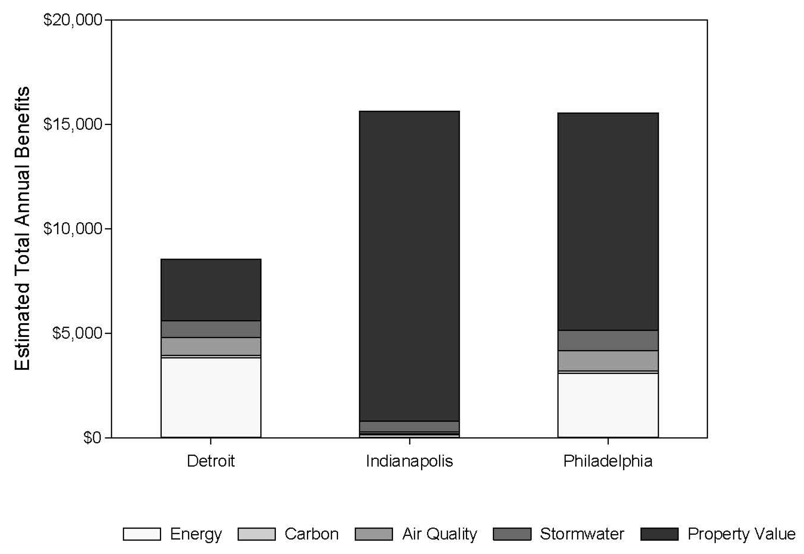
3.1.1. Current Benefits

Based on estimates from i-Tree, these 4059 re-inventoried trees provide a total of $46,377 in annual benefits. The value ranged from $8.91 per tree in Detroit to $20.25 per tree in Indianapolis (Table 6). At the time of re-inventory, the cumulative benefits provided by the sample trees (i.e., the sum of the annual benefits provided each year since planting) ranged from $17,096 in Detroit to $31,268 in Indianapolis (Table 6).
Property value benefits were the predominant benefit type in Indianapolis and Philadelphia, while energy benefits predominated in Detroit (Figure 2). Ninety-five percent of estimated annual benefits in Indianapolis were property value benefits because property value increase is the predominant benefit type in the Lower Midwest climate zone i-Tree models.

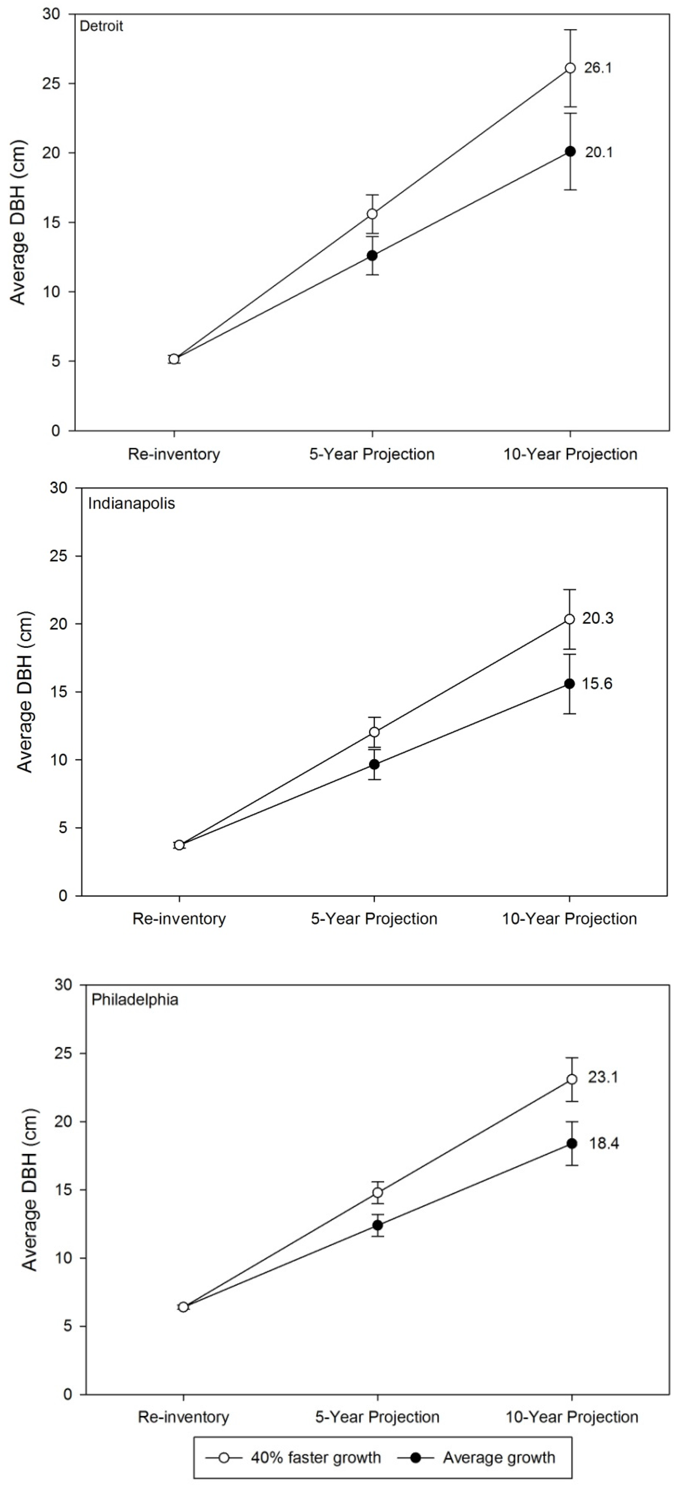
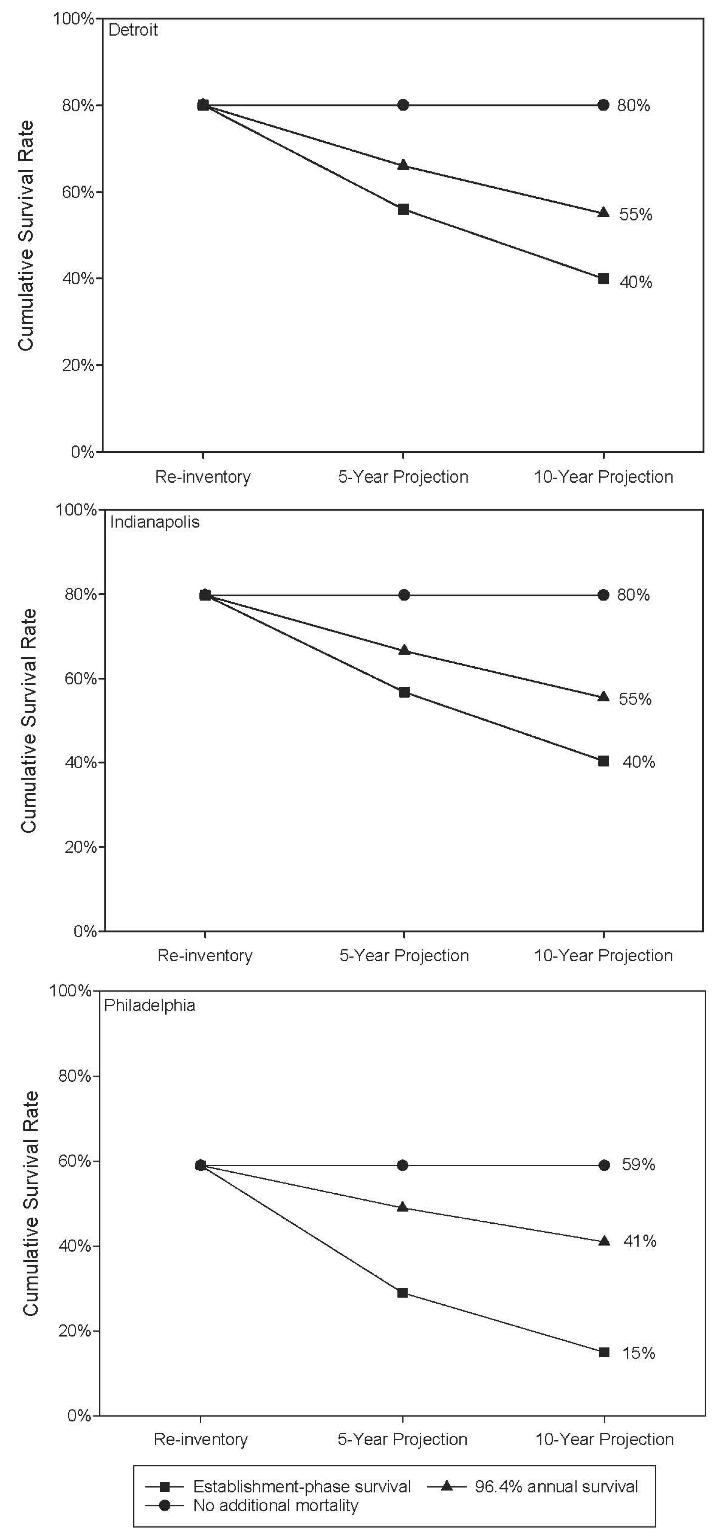
3.1.2. Growth and Survival Rates for Each City

The annual and cumulative survival rates were similar for Detroit and Indianapolis and lower for Philadelphia (Table 7). Relative growth rate ranged from 1.18 cm/year in Indianapolis to 1.48 cm/year in Detroit.

3.2. Projected Populations

The three different annual survival scenarios result in different proportions of trees remaining in the sample population 5 and 10 years in the future (Figure 3). With continued establishment-phase annual survival of 93% in Detroit and Indianapolis, only 40% of the planted trees in those cities will be alive in 10 years, compared to 80% of planted trees alive in 10 years with no additional mortality. With continued establishment-phase annual survival of 87% in Philadelphia, only 29% of planted trees will be alive in 5 years and only 15% will be alive in 10 years, compared to 59% of planted trees alive in 10 years with no additional mortality.
The two different growth scenarios (average vs. 40% faster growth) resulted in different average DBHs 5 and 10 years in the future (Figure 4). For each study city, the difference between the two growth rates is an approximately 2.5 cm difference in average DBH after 5 years and an approximately 5 cm difference in average DBH after 10 years.

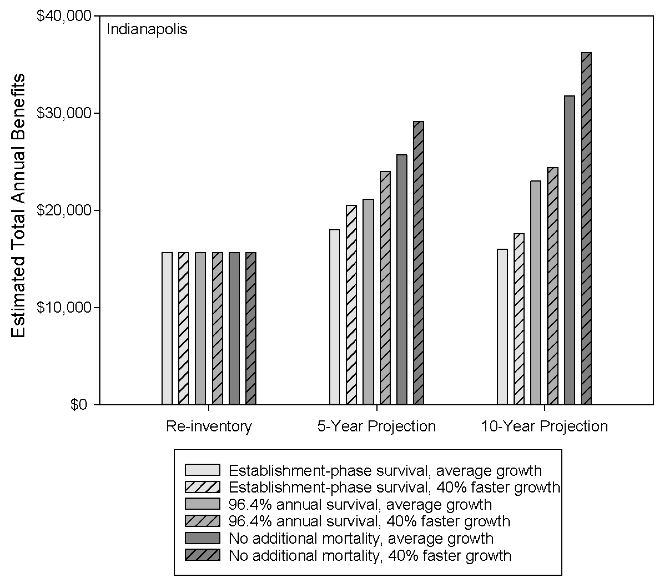
3.3. Projected Annual Benefits

3.3.1. Effect of Survival Scenario

The survival scenarios had a larger effect on projected total annual benefits than the growth scenarios. For both Detroit and Indianapolis, the no additional mortality scenario resulted in double the amount of projected total annual benefits of the establishment-phase survival scenario in the 10-year projection (Figure 5, Table 8). The difference was even more apparent for Philadelphia, where the no additional mortality scenario resulted in 3.5 times the amount of projected total annual benefits of the establishment-phase survival scenario in the 10-year projection (Table 8).
If the tree populations maintain the establishment-phase annual survival rates and the average growth rates continue, high tree mortality results in fewer trees conferring benefits; thus, the projected populations in Indianapolis and Philadelphia provide fewer benefits in the future (Figure 5). However, if the tree populations maintain an annual survival rate of 96.4%, the total annual benefits provided by the trees can be expected to increase over the next 10 years. If no more trees die, the total annual benefits provided by the tree populations can be expected to double in the next 10 years (Figure 5).

3.3.2. Effect of Growth Scenario

The growth rate scenarios had an effect on projected total annual benefits, but the effect was less pronounced than the effect of the survival scenario. For Indianapolis, average growth and no additional mortality resulted in $31,798 in total annual benefits in 10 years, while 40% faster growth and no additional mortality resulted in $36,209 in total annual benefits in 10 years (Figure 5, Table 8). The growth scenario had a bigger effect in Detroit, where average growth and no additional mortality resulted in $32,476 in total annual benefits in 10 years, while 40% faster growth and no additional mortality resulted in $42,972 in total annual benefits in 10 years (Table 8).

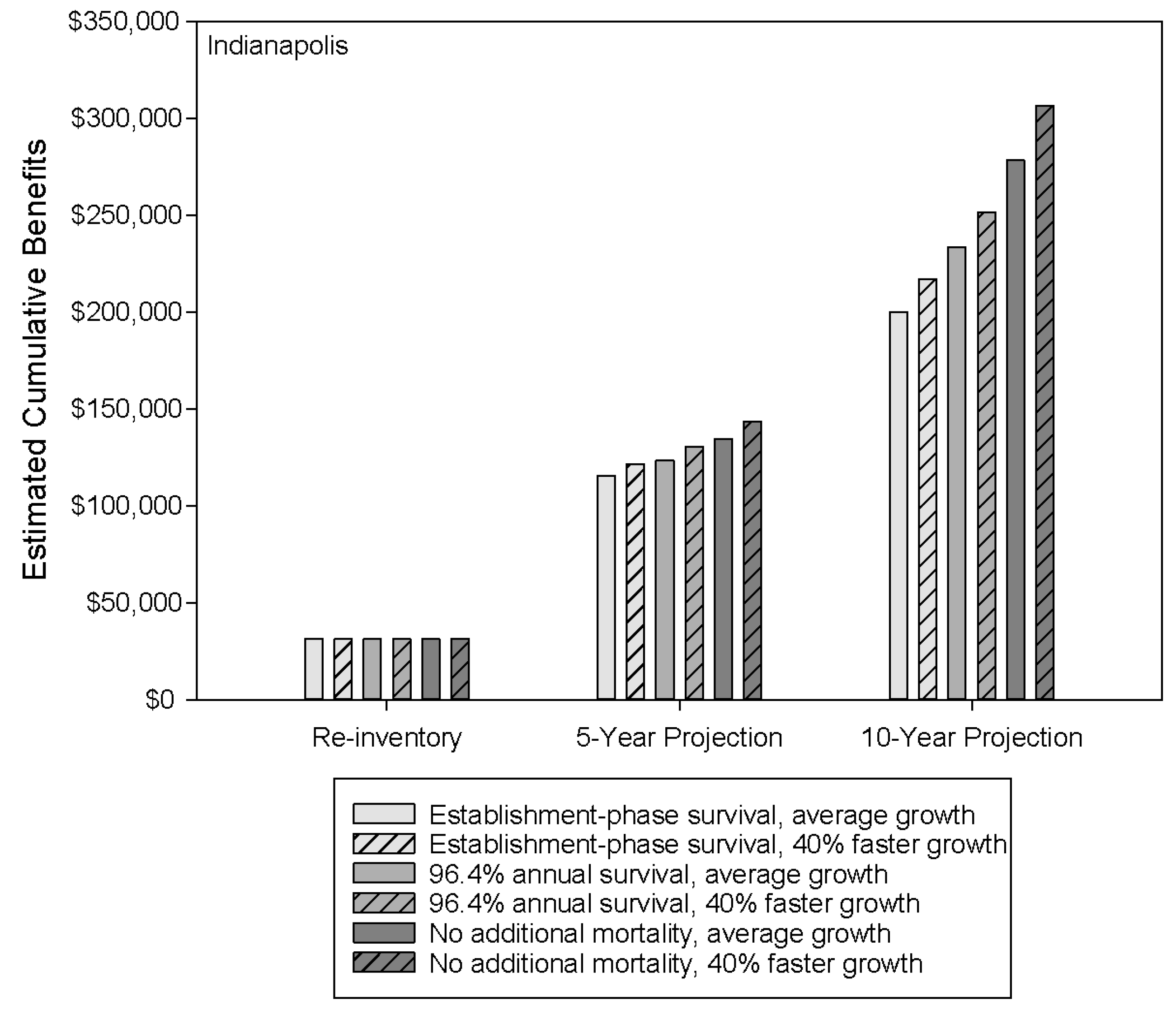
3.4. Projected Cumulative Benefits

Due to their additive nature, cumulative benefits increase substantially when the tree populations are projected into the future (Figure 6). Cumulative benefits increase by a factor of roughly 4 from the time of re-inventory to the 5-year projection, and then double again from the 5- to 10-year projection (Figure 6). Projected cumulative benefits in 10 years range from $154,000 to $271,000 in Detroit, from $200,000 to $307,000 in Indianapolis, and from $158,000 to $320,000 in Philadelphia (Table 9).

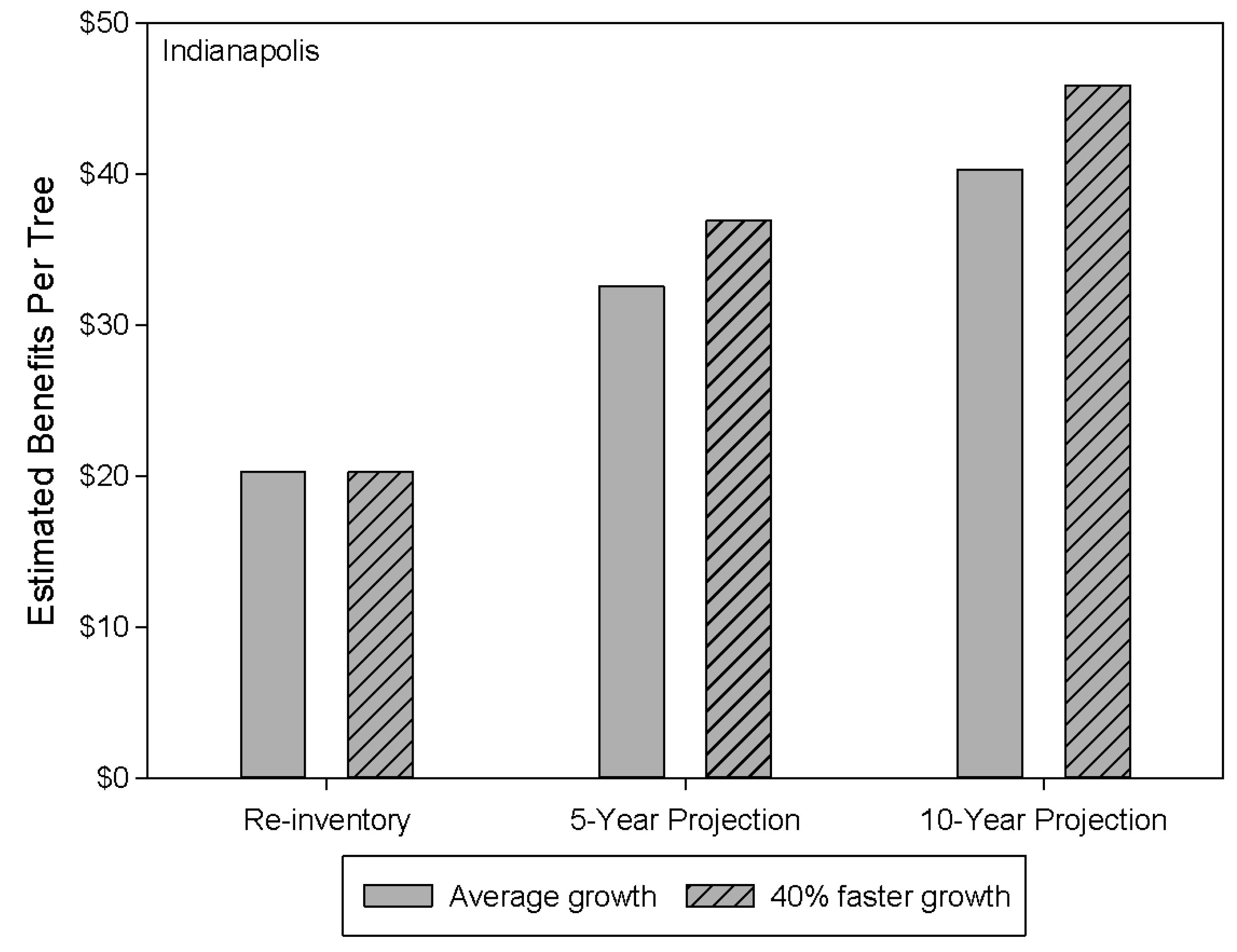
3.5. Projected Per-Tree Benefits

The average benefits per tree reflect the effect of tree size in determining future benefits. For all cities studied, faster growth results in higher average benefits per tree (Figure 7, Table 10). Under average growth conditions, the average value per tree 10 years in the future ranges from $34.87 (Philadelphia) to $40.30 (Indianapolis); the average value under 40% faster growth conditions ranges from $43.22 (Philadelphia) to $46.26 (Detroit).

3.6. Estimated Costs and Net Benefits

The i-Tree regional community tree guides estimate the average costs per tree, assuming a 40-year lifetime, to be $34/year for a large public tree in the Northeast [9] and $24/year for a large public tree in the Lower Midwest [8]. Using these estimated annual costs, the average annual benefits (Table 10) exceed average annual costs (i.e., net annual benefits are positive) after 13–15 years of growth (the 10-year projection) in Detroit and Philadelphia and after 8–10 years of growth (the 5-year projection) in Indianapolis.
Keep Indianapolis Beautiful, Inc. (Indianapolis, IN, USA) estimates their average per-tree costs are $100 per tree for planting plus $100 per year of watering for a total of $300 per tree for a tree watered for a 2-year establishment period (personal communication, N. Faris (Keep Indianapolis Beautiful, Inc.), 21 September 2015). Using this estimated cumulative per-tree cost, the net benefits per planted tree in Indianapolis are still negative after 13–15 years of growth, even with no additional mortality and 40% faster than average growth (Table 11).

4. Discussion

4.1. Future Benefit Increases

The total benefits provided by the sample of planted trees may increase or decrease depending on the survival rate in the future. These street trees can be expected to provide increasing annual benefits during the next 5–10 years if the annual survival rate is higher than the 93% annual survival measured during the establishment period. However, our projections show that with continued 93% or lower annual survival, the increase in annual benefits from tree growth will not be able to make up for the loss of benefits as trees die. This means that estimated total annual benefits from the populations of trees will decrease between the 5-year projection and the 10-year projection for Indianapolis and Philadelphia (Figure 5). In contrast, with higher survival rates, the benefits provided by the populations of trees can be expected to increase over the next 10 years in all cities (Figure 5). Somewhere between 93% and 96.4% annual survival represents the “tipping point” where the benefits added due to growth exceed the loss of benefits due to mortality.

4.2. Comparison of Results among Cities

The general patterns in how benefits change over time are not universally applicable across all cities studied. Notably, the estimated total annual benefits provided by the street tree population in 2014 in Detroit were substantially lower than the benefit estimates for the other cities. This difference is the result of a much lower average home resale value in Detroit ($37,000 compared to $128,000 and $155,000 for Indianapolis and Philadelphia, respectively). The unimportance of property value benefits in Detroit relative to other cities is likely responsible for the different trend in benefits over time in Detroit (namely, no decrease in estimated benefits from 5-year projection to 10-year projection, even in the low survival scenario). The trees in Detroit also had a higher growth rate than the trees in Indianapolis and Philadelphia (1.48 cm/year compared to 1.18 and 1.19 cm/year, respectively; Table 7), so growth was more able to make up for tree mortality.
In addition, the cities are located in different i-Tree climate zones, which affects how the modeled populations respond to variations in growth. In particular, the i-Tree climate zone affects how property value benefits are modeled for large trees. In the Northeast climate zone (which includes Detroit and Philadelphia), property value benefits and total benefits increase linearly with tree size, while in the Lower Midwest climate zone (which includes Indianapolis), property value benefits start to decrease after the tree reaches a DBH of 30 cm (12 inches) and total annual benefits do not increase any more beyond a DBH of 60 cm (24 inches) (Figure 8). These differences are an artifact of the limited data collected in the different climate zones (i.e., in one reference city per zone) and may or may not actually be representative of how street trees grow across the region.

4.3. Effect of Survival vs. Growth Rate

Our results indicate that tree survival is more important than growth for providing future benefits. This is a particularly relevant finding given the lack of follow-up on tree success (survival and/or growth) in many tree-planting programs/campaigns. Street tree survival rates observed 3–5 years post-planting in our study are not particularly high compared to other results in the literature [30,36,37] (see Table 12 for comparison). As a population, the planted street trees in this study will not provide many more benefits 10 years in the future if establishment-phase annual survival rates continue. However, if the annual survival rate increases modestly to 96.4%, a reasonable expectation since most mortality is expected during the first years after transplanting, the populations will provide between $22,564 (Detroit) and $24,484 (Philadelphia) in total annual benefits in 10 years, even if the growth rates do not increase (Table 8).

4.4. Maintenance Costs and Net Benefits of Recently Planted Street Trees

Whether the net benefits are positive after 13–15 years of tree growth depends on the cost calculation used; when annual benefits per tree are compared to the annual costs per tree from the i-Tree community tree guides, the net benefits are positive. However, this comparison does not include the costs for trees that were planted and then died—the per-tree costs would be higher if money spent on dead trees were included. In contrast, our comparison of cumulative benefits to the cumulative costs of planting and watering the trees shows that net benefits per planted tree are still negative after 13–15 years of growth for all tested scenarios (Table 11). Clearly, investing in the planting and watering of trees is a long-term investment. However, this back-of-the-envelope calculation implies that increasing survival and growth rates as much as possible decreases the payback period (or, amount of time until net benefits become positive and the investment in planting and maintenance is paid back as tree benefits) for a population of planted trees.
If even higher-than-measured growth rates cannot make up for tree mortality, efforts to maintain street trees that survive in the landscape are important. In order to get the best return on investment from planting street trees, follow-up maintenance and monitoring to ensure high survival rates are necessary. For instance, Boyce [38] observed that mortality rates were three times lower (that is, survival rates were higher) for trees with “stewards” (designated groups or individuals assigned to provide maintenance for a tree, including watering and tree pit care) than for trees without stewards. Gilman [39] compared the planting and maintenance costs of irrigated and not irrigated trees and found that mortality of non-irrigated trees resulted in higher costs per live tree 1 year after transplanting. This implies that a population of irrigated trees with low mortality rates should yield higher total net benefits than a population of non-irrigated trees with lower planting and maintenance costs but higher mortality rates (see Vogt, et al. [10] for a net benefits calculation using data from Gilman [39]).

4.5. Other Costs of Street Trees

The cost estimates from the i-Tree community tree guides [8,9] include planting, pruning, removal/disposal, infrastructure damage, irrigation, cleanup, liability/legal, and administrative costs. In addition, biogenic VOC and CO2 emissions associated with trees are accounted for in the air quality and carbon benefit estimates, respectively [8,9]. Although these cost estimates do not include every possible costs associated with trees, we believe they represent those costs most typically associated with young, planted street trees.

4.6. Comparison to Similar Studies

McPherson and colleagues [40] modeled high and low survival scenarios 35 years into the future for Los Angeles’s Million Trees LA tree-planting campaign, and found that a drop from “high” survival (1% annual mortality for the first 5 years and 0.5% annual mortality thereafter) to “low” survival (5% annual mortality for the first 5 years and 2% annual mortality thereafter) resulted in a 30% decrease in cumulative benefits after 35 years. A follow up study by McPherson [41] found that survival of selected street trees five years after planting more closely matched the low survival scenario from [40]. These results provide evidence that studies predicting the benefits of tree-planting programs (e.g., [40]) can easily overestimate the actual survival rates (and thus, future benefits) of planted trees.
In a similar study conducted in New York City to evaluate the MillionTreesNYC initiative, Morani and colleagues [42] predicted that if 100,000 trees per year were planted over the course of 10 years (thus reaching the goal of 1 million trees planted), the trees would remove 11,000 tons of air pollutants over the next 100 years if they maintain an annual mortality rate of 4% or less. However, the amount of air pollutants removed would drop to 3000 tons over the next 100 years if the annual mortality rate increased to 8% per year [42]. Other researchers have also discussed the relative importance of mortality rates over growth rates for determining future tree benefits. For example, Strohbach and colleagues [43] found that a modeled tree population sequesters 70% less carbon over its 50-year lifetime when annual mortality increases from 0.5% to 4%.

4.7. Limitations of This Study

There are two main sources of uncertainty in this analysis: the uncertainty in projecting survival and growth rates into the future, and the uncertainty in using i-Tree Streets to assign monetary values to the benefits provided by a population of street trees. We have tried to address the first source of uncertainty by modeling different survival and growth scenarios without making predictions as to which scenario is the most likely outcome; few studies have examined long-term growth or survival of city trees (but see [30,37,41,44,45,46,47,48]), and even fewer have examined species-specific growth or survival (e.g., [34]). The second source of uncertainty is more difficult to address. We have done our due diligence in investigating how i-Tree Streets estimates monetized benefits so we are aware of its sensitivities, but there are many aspects of the benefit estimates that are beyond our control. We acknowledge that the benefits experienced by the residents of these cities are likely different from the benefit estimates presented here, but these rough estimates are the best we can do with the tools available to us.
Other sources of uncertainty include our use of approximate caliper-at-planting rather than actual measurements and citywide growth rates rather than species-specific growth rates. These limitations are the result of the tradeoff between having a large sample size and having more details on each individual tree—we are willing to use approximate caliper-at-planting because it is what our nonprofit partners could provide for the number of trees we needed for this study. We chose not to use species-specific growth rates because it was unclear whether calculating growth rates by species or genus would provide more accurate growth rates, given the limitations in precision of caliper-at-planting data. Finally, we know there are problems with estimating benefits for large trees in i-Tree (see Figure 8), but this is less of a concern given that most of the trees in the 10-year projections were between 20 and 25 cm (8–10 inches) DBH.

Limitations of i-Tree

Perhaps the biggest limitations of this study are the limitations imposed by i-Tree. i-Tree calculates several important types of tree benefits: increased property values, air quality, carbon sequestration, energy savings, and stormwater mitigation. However, this leaves out many additional benefits that are less easily monetized, such as increased retail sales [49], reduced crime rates [3,4,5], and improved human health and well-being [6,7]. Furthermore, there are additional costs in time, money, and resources of managing trees that would need to be included in any true cost-benefit analysis or calculation of net benefits [12] (see Section 1.3 or [10] for a full discussion of costs associated with trees).
The i-Tree benefit estimates are not perfect; they involve many assumptions about how urban trees grow, the similarity of performance of different tree species, and the value urban trees will provide in different contexts [8,9]. Nowak and colleagues [50] named reliance on models to estimate functions of the urban forest, the potential estimation error of the biomass equations used, and the lack of data on ornamental and tropical tree species as some of the limitations of the UFORE model (used in i-Tree Eco, a sibling module of Streets in the i-Tree family). Dobbs and colleagues [51] also outlined some limitations of the UFORE model, including the limited data incorporated into the models, the bias towards species native to the northern U.S., and the difficulty of obtaining representative samples in the urban environment. The STRATUM model (used in i-Tree Streets) is subject to many of the same limitations. Given these limitations, the benefit estimates generated by i-Tree should be viewed as estimates only, and should not be interpreted as justification for investing in trees at the expense of investing in other types of urban infrastructure (i.e., stormwater and sewer systems).

5. Conclusions

The main management implication of this study is that ensuring the survival of planted street trees is most important for providing future benefits; each dead tree represents a loss of $40–$50 in annual benefits for the city each year after the tree dies, while faster growth only increases the annual benefits per tree by $11.30 at the most (Table 10). This increase is not inconsequential, but also is not as dramatic as the increase in benefits gained from increasing annual survival. The differences in future total annual benefits between the establishment-phase survival rate scenarios and the no additional mortality scenarios (Figure 5) are striking, and indicate that tree-planting campaigns that do not track the survival of planted trees may be significantly overestimating the benefits provided by the trees if they assume 100% survival. If planting and establishment (i.e., watering) costs are considered and net benefits are calculated (Table 11), high survival rates have the potential to decrease payback time for a population of planted trees (when average net benefits per planted tree become positive). The results of this study provide evidence for the importance of tracking the survival and growth of planted trees. If “success” is below expectations, planting and/or maintenance activities should be modified in the future to improve survival and/or growth rates as possible. Additionally, we have learned that high survival rates during the early establishment period (years 1–3) are critical to maximizing benefits; conversely, low initial survival rates can have a negative impact from which it is impossible to recover. High survival rates (greater than 96% annually) are necessary to ensure that the trees are able to provide the maximum amount of benefits possible over their lifetime.

Acknowledgments

A version of this research was presented at the 2015 International Society of Arboriculture Annual Conference and Trade Show, in the Arboriculture Research and Education Academy (AREA) student presentations; SEW received an AREA Travel Grant that enabled this presentation. The U.S. Forest Service (USFS) National Urban and Community Forestry Advisory Council (NUCFAC) and the USFS Northern Research Station provided major funding for the project from which tree survival and growth data used in this paper emerged. Partnerships with Alliance for Community Trees (ACTrees) and several ACTrees member organizations (Keep Indianapolis Beautiful, Pennsylvania Horticultural Society, The Greening of Detroit, Trees Atlanta and Forest ReLeaf of Missouri) made the aforementioned USFS grants possible. Additional funding was provided by: the Indiana University Office of Sustainability and the Garden Club of America, and additional support was provided by: The Vincent and Elinor Ostrom Workshop in Political Theory and Policy Analysis, the Center for the Study of Institutions, Population and Environmental Change, and the School of Public and Environmental Affairs, all at Indiana University Bloomington. Most importantly, we are grateful to the additional team members who participated in the larger research effort on which this paper was derived: Shannon Lea Watkins, Sarah K. Mincey, Rachael Bergmann, and Lynne Westphal. We are also grateful for the comments of four anonymous reviewers and the journal editor that significantly improved this paper.

Author Contributions

B.F. and J.V. conceived and designed the broader experiment on which this project was based; S.W. and B.F. conceived and designed the experiments specific to this project; S.W. performed the experiments and analyzed the data; S.W., J.V. and B.F. wrote the paper.

Conflicts of Interest

The authors declare no conflict of interest. The funding sponsors had no role in the design of the study; in the collection, analyses, or interpretation of data; in the writing of the manuscript, and in the decision to publish the results.

References

  1. Xiao, Q.; McPherson, E.G.; Simpson, J.R.; Ustin, S.L. Rainfall interception by Sacramento’s urban forest. J. Arboric. 1998, 24, 235–244. [Google Scholar]
  2. Nowak, D.J.; Crane, D.E.; Stevens, J.C. Air pollution removal by urban trees and shrubs in the United States. Urban For. Urban Green. 2006, 4, 115–123. [Google Scholar] [CrossRef]
  3. Donovan, G.H.; Prestemon, J.P. The effect of trees on crime in Portland, Oregon. Environ. Behav. 2012, 44, 3–30. [Google Scholar] [CrossRef]
  4. Garvin, E.C.; Cannuscio, C.C.; Branas, C.C. Greening vacant lots to reduce violent crime: A randomised controlled trial. Inj. Prev. 2012, 19, 198–203. [Google Scholar] [CrossRef] [PubMed]
  5. Troy, A.; Grove, M.J.; O’Neil-Dunne, J. The relationship between tree canopy and crime rates across an urban-rural gradient in the greater Baltimore region. Landsc. Urban Plan. 2012, 106, 262–270. [Google Scholar] [CrossRef]
  6. South, E.C.; Kondo, M.C.; Cheney, R.A.; Branas, C.C. Neighborhood blight, stress, and health: A walking trial of urban greening and ambulatory heart rate. Am. J. Public Health 2015, 105, e1–e5. [Google Scholar] [CrossRef] [PubMed]
  7. Bell, J.F.; Wilson, J.S.; Liu, G.C. Neighborhood greenness and 2-year changes in body mass index of children and youth. Am. J. Prev. Med. 2008, 35, 547–553. [Google Scholar] [CrossRef] [PubMed]
  8. Peper, P.J.; McPherson, E.G.; Simpson, J.R.; Vargas, K.E.; Xiao, Q. Lower Midwest Community Tree Guide: Benefits, Costs, and Strategic Planting; US Department of Agriculture Forest Service, Pacific Southwest Research Station: Albany, CA, USA, 2009. [Google Scholar]
  9. McPherson, E.G.; Simpson, J.R.; Peper, P.J.; Gardner, S.L.; Vargas, K.E.; Xiao, Q. Northeast Community Tree Guide: Benefits, Costs, and Strategic Planting; United States Department of Agriculture Forest Service, Pacific Southwest Research Station: Albany, CA, USA, 2007. [Google Scholar]
  10. Vogt, J.M.; Hauer, R.J.; Fischer, B.C. The costs of maintaining and not maintaining trees: A review of the urban forestry and arboriculture literature. Arboric. Urban For. 2015, 41, 293–322. [Google Scholar]
  11. Von Dohren, P.; Haase, D. Ecosystem disservices research: A review of the state of the art with a focus on cities. Ecol. Indic. 2015, 52, 490–497. [Google Scholar] [CrossRef]
  12. Escobedo, F.J.; Kroeger, T.; Wagner, J.E. Urban forests and pollution mitigation: Analyzing ecosystem services and disservices. Environ. Pollut. 2011, 159, 2078–2087. [Google Scholar] [CrossRef] [PubMed]
  13. Randrup, T.B.; McPherson, E.G.; Costello, L.R. Tree root intrusion in sewer systems: Review of extent and costs. J. Infrastruct. Syst. 2001, 7, 26–31. [Google Scholar] [CrossRef]
  14. McPherson, E.G.; Peper, P.J. Infrastructure repair costs associated with street trees in 15 cities. In Trees and Building Sites; Watson, G., Neely, D., Eds.; International Society of Arboriculture: Savoy, IL, USA, 1995; pp. 49–64. [Google Scholar]
  15. Posner, R.A. Cost-benefit analysis: Definition, justification, and comment on conference papers. J. Leg. Stud. 2000, 29, 1153–1177. [Google Scholar] [CrossRef]
  16. i-Tree Streets. i-Tree Software Suite v6.0.7. n.d. Available online: http:/www.itreetools.org (accessed on 29 August 2014).
  17. i-Tree Streets User’s Manual v5.0. n.d. Available online: http://www.itreetools.org/resources/manuals/Streets_Manual_v5.pdf (accessed on 29 August 2014).
  18. Bloomington Urban Forestry Research Group. About the Bloomington Urban Forestry Research Group (BUFRG) at CIPEC. Available online: https://www.indiana.edu/~cipec/research/bufrg_about.php (accessed on 10 March 2016).
  19. Bloomington Urban Forestry Research Group. Urban Forestry in 5 U.S. Cities—Ecological & Social Outcomes of Neighborhood & Nonprofit Tree Planting: NUCFAC Grant. Available online: https://www.indiana.edu/~cipec/research/bufrgproj_nucfac.php (accessed on 10 March 2016).
  20. Vogt, J.M.; Fischer, B.C. A protocol for citizen science monitoring of recently-planted urban trees. Cities Environ. 2014, 7, 4. [Google Scholar]
  21. Vogt, J.M.; Mincey, S.K.; Fischer, B.C.; Patterson, M. Planted Tree Re-Inventory Protocol; Version 1.1; Bloomington Urban Forestry Research Group at the Center for the Study of Institutions, Population and Environmental Change, Indiana University: Bloomington, IN, USA, 2014. [Google Scholar]
  22. StataCorp. Stata Statistical Software: Release 13; StataCorp LP: College Station, TX, USA, 2013. [Google Scholar]
  23. Peper, P.J.; McPherson, E.G.; Mori, S.M. Equations for predicting diameter, height, crown width, and leaf area of San Joaquin Valley street trees. J. Arboric. 2001, 27, 306–317. [Google Scholar]
  24. Peper, P.J.; McPherson, E.G.; Mori, S.M. Predictive equations for dimensions and leaf area of coastal Southern California street trees. J. Arboric. 2001, 27, 169–180. [Google Scholar]
  25. Xiao, Q.; McPherson, E.G.; Ustin, S.L.; Grismer, M.E.; Simpson, J.R. Winter rainfall interception by two mature open-grown trees in Davis, California. Hydrol. Process. 2000, 14, 763–784. [Google Scholar] [CrossRef]
  26. Anderson, L.M.; Cordell, H.K. Influence of trees on residential property values in Athens, Georgia (USA): A survey based on actual sales prices. Landsc. Urban Plan. 1988, 15, 153–164. [Google Scholar] [CrossRef]
  27. DTE Energy. Your Natural Gas Pricing Options. Available online: https://www2.dteenergy.com/wps/wcm/connect/11919444-45e5-4a7c-afab-33d6db22b198/Gas+Rate+9-14_internet.pdf?MOD=AJPERES (accessed on 31 October 2014).
  28. Citizens Energy Group. Gas Rate No. D2. Available online: http://www.citizensenergygroup.com/ratesriders/RateNo%20D2%20ResHeatDelivery%20-%20eff.%209-6-11.pdf (accessed on 31 October 2014).
  29. Pennsylvania Public Utilities Commission. Natural Gas Shopping Tool. Available online: http://www.puc.pa.gov/consumer_info/natural_gas/natural_gas_shopping/gas_shopping_tool.aspx (accessed on 31 October 2014).
  30. Roman, L.A.; Scatena, F.N. Street tree survival rates: Meta-analysis of previous studies and application to a field survey in Philadelphia, PA, USA. Urban For. Urban Green. 2011, 10, 269–274. [Google Scholar] [CrossRef]
  31. Brand, D.G. The establishment of boreal and sub-boreal conifer plantations: An integrated analysis of environmental conditions and seedling growth. For. Sci. 1991, 37, 68–100. [Google Scholar]
  32. Samyn, J.; de Vos, B. The assessment of mulch sheets to inhibit competitive vegetation in tree plantations in urban and natural environment. Urban For. Urban Green. 2002, 1, 25–37. [Google Scholar] [CrossRef]
  33. Richards, N.A. Modeling survival and consequent replacement needs in a street tree population. J. Arboric. 1979, 5, 251–255. [Google Scholar]
  34. Miller, R.H.; Miller, R.W. Survival of selected street tree taxa. J. Arboric. 1991, 17, 185–191. [Google Scholar]
  35. Gilman, E.F.; Black, R.J.; Dehgan, B. Irrigation volume and frequency and tree size affect establishment rate. J. Arboric. 1998, 24, 1–9. [Google Scholar]
  36. Thompson, J.R.; Nowak, D.J.; Crane, D.E.; Hunkins, J.A. Iowa, US, communities benefit from a tree-planting program: Characteristics of recently planted trees. J. Arboric. 2004, 30, 1–10. [Google Scholar]
  37. Lu, J.W.T.; Svendsen, E.S.; Campbell, L.K.; Greenfeld, J.; Braden, J.; King, K.L.; Falxa-Raymond, N. Biological, social, and urban design factors affecting young street tree mortality in New York City. Cities Environ. 2010, 3, 1–15. [Google Scholar]
  38. Boyce, S. It takes a stewardship village: Effect of volunteer tree stewardship on urban street tree mortality rates. Cities Environ. 2010, 3, 1–8. [Google Scholar]
  39. Gilman, E.F. Effect of nursery production method, irrigation, and inoculation with mycorrhizae-forming fungi on establishment of Quercus virginiana. J. Arboric. 2001, 27, 30–39. [Google Scholar]
  40. McPherson, E.G.; Simpson, J.R.; Xiao, Q.; Wu, C. Los Angeles 1-Million Tree Canopy Cover Assessment; US Department of Agriculture Forest Service, Pacific Southwest Research Station: Albany, CA, USA, 2008. [Google Scholar]
  41. McPherson, E.G. Monitoring Million Trees LA: Tree performance during the early years and future benefits. Arboric. Urban For. 2014, 40, 285–300. [Google Scholar]
  42. Morani, A.; Nowak, D.J.; Hirabayashi, S.; Calfapietra, C. How to select the best tree planting locations to enhance air pollution removal in the MillionTreesNYC initiative. Environ. Pollut. 2011, 159, 1040–1047. [Google Scholar] [CrossRef] [PubMed]
  43. Strohbach, M.W.; Arnold, E.; Haase, D. The carbon footprint of urban green space—A life cycle approach. Landsc. Urban Plan. 2012, 104, 220–229. [Google Scholar] [CrossRef]
  44. Sklar, F.; Ames, R.G. Staying alive: Street tree survival in the inner-city. J. Urban Aff. 1985, 7, 55–66. [Google Scholar] [CrossRef]
  45. Roman, L.A.; Battles, J.J.; McBride, J.R. Determinants of establishment survival for residential trees in Sacramento County, CA. Landsc. Urban Plan. 2014, 129, 22–31. [Google Scholar] [CrossRef]
  46. Roman, L.A.; Battles, J.J.; McBride, J.R. The balance of planting and mortality in a street tree population. Urban Ecosyst. 2013, 17, 387–404. [Google Scholar] [CrossRef]
  47. Jack-Scott, E.; Piana, M.; Troxel, B.; Murphy-Dunning, C.; Ashton, M.S. Stewardship success: How community group dynamics affect urban street tree survival and growth. Arboric. Urban For. 2013, 39, 189–196. [Google Scholar]
  48. Koeser, A.; Hauer, R.; Norris, K.; Krouse, R. Factors influencing long-term street tree survival in Milwaukee, WI, USA. Urban For. Urban Green. 2013, 12, 562–568. [Google Scholar] [CrossRef]
  49. Wolf, K.L. Business district streetscapes, trees, and consumer response. J. For. 2005, 103, 396–400. [Google Scholar]
  50. Nowak, D.J.; Crane, D.E.; Stevens, J.C.; Hoehn, R.E.; Walton, J.T.; Bond, J. A ground-based method of assessing urban forest structure and ecosystem services. Arboric. Urban For. 2008, 34, 347–358. [Google Scholar]
  51. Dobbs, C.; Escobedo, F.J.; Zipperer, W.C. A framework for developing urban forest ecosystem services and goods indicators. Landsc. Urban Plan. 2011, 99, 196–206. [Google Scholar] [CrossRef]
Figure 1. Hypothetical benefits and costs over a tree’s lifetime [10]. Used with the permission of the International Society of Arboriculture.
Forests 07 00065 g001
Figure 2. Estimated total annual benefits, by type, for each city based on 2014 re-inventory data.
Forests 07 00065 g002
Figure 3. Cumulative survival rates of re-inventoried trees in 5 and 10 years with the three different survival scenarios in the three study cities.
Forests 07 00065 g003
Figure 4. Average diameter at breast height (DBH) at re-inventory and projected 5 and 10 years into the future with average growth and 40% faster growth for each study city. Error bars represent 95% confidence intervals based on the standard error of the growth rate in each city.
Forests 07 00065 g004
Figure 5. Estimated total annual benefits of re-inventoried trees in Indianapolis at the time of re-inventory and projected 5 and 10 years into the future.
Forests 07 00065 g005
Figure 6. Estimated total cumulative benefits of re-inventoried trees in Indianapolis at the time of re-inventory and projected 5 and 10 years into the future.
Forests 07 00065 g006
Figure 7. Estimated annual benefits per tree in Indianapolis at the time of re-inventory and projected 5 and 10 years into the future with average growth and 40% faster growth.
Forests 07 00065 g007
Figure 8. Annual benefits per tree by size for a hypothetical sugar maple (Acer saccharum) in the Northeast and Lower Midwest climate zones.
Forests 07 00065 g008
Table 1. Explanation of overall condition ratings used in the planted tree re-inventory protocol [21].
RatingExplanation
GoodFull canopy, minimal to no mechanical damage to trunk, no branch dieback over 5 cm (2′′) in diameter, no suckering (root or water sprouts), form is characteristic of species.
FairThinning canopy, new growth in medium to low amounts, tree may be stunted, significant mechanical damage to trunk (new or old), insect/disease is visibly affecting the tree, form not representative of species, premature fall coloring on foliage, needs training pruning.
PoorTree is declining, visible dead branches over 5 cm (2′′) in diameter in canopy, significant dieback of other branches in inner and outer canopy, severe mechanical damage to trunk usually including decay from damage, new foliage is small, stunted or minimum amount of new growth, needs priority pruning of dead wood.
DeadStanding dead tree, no signs of life with new foliage, bark may be beginning to peel.
SproutsOnly a stump of a tree is present, with one or more water sprouts of 45 cm (18′′) or greater in height growing from the remaining stump and root system.
StumpOnly a stump remains, no water sprouts greater than 45 cm (18′′) high present.
ShrubExisting vegetation is a shrub growth habit rather than tree growth habit, either because a shrub-form was planted or because the species has been pruned into the shape of a shrub (e.g., many crape myrtle, Lagerstroemia sp.).
AbsentNo tree present, not even a stump remains visible in the location where the tree should have been; this category should also be used for trees that have obviously been replaced (are the incorrect species, much smaller than they should be given the planting date, etc.) and there is no evidence of the original tree.
Table 2. Reference cities and community tree guide citations for the i-Tree climate zone used for each study city.
Climate ZoneStudy CitiesReference CityCommunity Tree Guide Citation
Lower MidwestIndianapolis, INIndianapolis, INPeper, et al. 2009 [8]
NortheastDetroit, MI and Philadelphia, PAQueens, NYMcPherson, et al. 2007 [9]
Table 3. Time, calendar year, and age of trees at each timepoint used in benefit projections.
Time PointYearAge of Trees (Time in Ground)
Planting2009–20110
Re-inventory20143–5 years
Midpoint * 120176–8 years
5-year projection20198–10 years
Midpoint * 2202211–13 years
10-year projection202413–15 years
* Midpoints are only used in calculating cumulative benefits for 5- and 10-year projections and are not shown in tables and figures in the results.
Table 4. Combinations of survival and growth scenarios used in benefit projections.
SurvivalGrowth
Establishment-phaseAverage
Establishment-phase40% faster than average
96.4% annualAverage
96.4% annual40% faster than average
No additional mortalityAverage
No additional mortality40% faster than average
Table 5. Number of trees surveyed compared to the number of trees planted from 2009 to 2011 for the three study cities.
CityTotal Number of Trees Re-InventoriedNumber of Trees Planted 2009–2011Percent of Planted Trees Re-Inventoried
Detroit1241677718%
Indianapolis107611,29410%
Philadelphia1742689432%
100% of the trees in randomly selected block groups were inventoried in Detroit and Philadelphia, while 52% of trees were re-inventoried in Indianapolis. Data collection teams were instructed to inventory every other tree in a block group unless they estimated they would have sufficient time to inventory all planted trees.
Table 6. Summary of estimated total annual benefits, average annual benefits per tree, and cumulative benefits for the three study cities in 2014.
CityTotal Annual BenefitsAverage Annual Benefits Per TreeCumulative Benefits
Detroit$8,548$8.91$17,096
Indianapolis$15,635$20.25$31,268
Philadelphia$15,556$15.70$31,112
Table 7. Survival and growth of re-inventoried trees in the three study cities.
CityCumulative Survival RateAnnual Survival RateRelative Growth Rate
Detroit79%93%1.48 cm/year
Indianapolis80%93%1.18 cm/year
Philadelphia59%87%1.19 cm/year
Table 8. Projected total annual benefits of re-inventoried trees in Detroit, Indianapolis, and Philadelphia 10 years in the future with all combinations of survival and growth scenarios.
CityEstablishment-Phase Survival96.4% Annual SurvivalNo Additional Mortality
Average growth40% faster growthAverage growth40% faster growthAverage growth40% faster growth
Detroit$16,622$21,999$22,564$29,899$32,476$42,972
Indianapolis$16,004$17,616$23,021$24,424$31,798$36,209
Philadelphia$9,667$11,947$24,484$30,161$34,558$42,831
Table 9. Projected total cumulative benefits of re-inventoried trees in Detroit, Indianapolis, and Philadelphia 10 years in the future with all combinations of survival and growth scenarios (rounded to the nearest thousand).
CityEstablishment-Phase Survival96.4% Annual SurvivalNo Additional Mortality
Average growth40% faster growthAverage growth40% faster growthAverage growth40% faster growth
Detroit$154,000$184,000$181,000$219,000$221,000$271,000
Indianapolis$200,000$217,000$234,000$252,000$278,000$307,000
Philadelphia$158,000$173,000$238,000$268,000$280,000$320,000
Table 10. Estimated total annual benefits per tree 5 and 10 years in the future under average growth and 40% faster growth conditions in all study cities.
Average Growth40% Faster Growth
CityRe-Inventory5-Year Projection10-Year Projection5-Year Projection10-Year Projection
Detroit$8.91$21.88$34.96$26.97$46.26
Indianapolis$20.25$32.56$40.30$36.94$45.89
Philadelphia$15.70$25.01$34.87$28.76$43.22
Table 11. Cumulative benefits and net benefits per planted tree in Indianapolis, IN, 10 years in the future with all combinations of survival and growth scenarios.
Indianapolis (Per 1076 Planted Trees)Establishment-Phase Survival96.4% Annual SurvivalNo Additional Mortality
Average Growth40% Faster GrowthAverage Growth40% Faster GrowthAverage Growth40% Faster Growth
Cumulative benefits for all trees$200,000$217,000$234,000$252,000$278,000$307,000
Average cumulative benefits per planted tree$186$202$217$234$258$285
Net benefits per planted tree after 10 years−$114−$98−$83−$66−$42−$15
Table 12. Annual survival rates from other in situ studies of urban tree survival.
Annual Survival RateTime Since PlantingLocationStudy
87%3–5 yearsPhiladelphia, PAThis study
93%3–5 yearsDetroit, MI and Indianapolis, INThis study
94%3–4 years20 cities in Iowa[36]
95.5%2–10 yearsPhiladelphia, PA[30] (street tree survey)
95.6%2 yearsNew York City, NY[37]
94.9%–96.5%VariousVarious[30] (meta-analysis)

