The Dynamic Trend of Soil Water Content in Artificial Forests on the Loess Plateau, China

Abstract

Extensive vegetation restoration projects have been widely implemented on the Loess Plateau, China, since 1998. In addition, increasing attention has been paid to the influence of revegetation on soil water. However, the response of the soil water content (SWC) to vegetation construction and management has not been adequately studied. In this study, three types of typical artificial vegetation on level bench land were selected, including Pinus tabulaeformis Carr., Prunus sibirica L., and Hippophae rhamnoides Linn., with the natural grassland used as a control group in Wuqi County. The 0–160 cm SWC was monitored biweekly from August 2010 to June 2013 using a portable time domain reflectometry system. The serial autocorrelation test, Mann–Kendall trend test, and prewhitening Mann–Kendall test were employed to systematically analyze the trends in soil water dynamics. The results show that the SWC of the three selected artificial forests/shrub had a significant accumulation process in the 0–160 cm profile during the monitoring period, whereas such an increasing tendency was not observed for natural grassland. Furthermore, the greatest responses were observed in the Pinus tabulaeformis Carr. plantation.

1. Introduction

To accelerate the process of vegetation restoration, the Grain-for-Green project was implemented on the loess slope of northern Shaanxi province, and a vast area of plantations has been constructed since 1998 [1,2]. For these types of artificial forests, the spatiotemporal variation of the soil water is very pronounced [3] because of antecedent precipitation, surface runoff, surface evaporation, transpiration, soil characteristics, plant root absorption, and so on [4,5]. Some studies have suggested that soil water plays a key role in plant growth [6,7], and it is likely to be a limiting factor for plant growth on the semiarid Loess Plateau, China [8]. Therefore, the effects of artificial forest construction on soil water dynamics are very important when implementing vegetation restoration projects in this area [9].

On the Loess Plateau, some researchers studied the relationship between soil water and vegetation restoration and found that the vegetation would excessively consume limited soil water resources [10], which would gradually deplete soil water, aggravate water scarcity, and even induce soil desiccation [10,11]. Soil water scarcity and desiccation have become very common in this semiarid area [12,13], especially in the artificial forest area [14,15]. The direct causes of soil water scarcity and desiccation may be climate warming [16] and decreasing precipitation [17]. Furthermore, other factors may have also resulted in this situation becoming more severe, such as improper selection of vegetation type [10,18], excessive community density [19], exorbitant productivity [12], and so on. However, Feng and Liu [20] studied the soil water content (SWC) of different land covers and stated that forests might increase the SWC. Therefore, the influence of plantations on the SWC of the Loess Plateau and its dynamic trend needs to be investigated using a systematic, long-term study.

Time series analysis with a general additive model, autoregressive (AR) model [21], autoregressive integrated moving average (ARIMA) model [22], and exponential smoothing model [23] have been used extensively in investigations on the trends in soil water dynamics [24], and were even used for forecasting the soil water dynamic tendency. These methods can be used to test the autocorrelation of SWC series [25], but are inadequate for the monotonic trend significance of SWC series [26]. The Mann–Kendall test (M–K test), originally presented by Mann [27] and Kendall [28], can be used to test the time series monotonic trend of the SWC [29,30]. The M–K test, a nonparametric statistical test method, is appropriate for time series without autocorrelation [31]. It has been widely used in significant studies on climate [32], hydrology [33], and vegetation [34], and used for a few monotonicity analyses of SWC series. However, antecedent SWC values always affect subsequent values [35]. In other words, there is serial autocorrelation in the SWC time series. To eliminate the influence of serial autocorrelation in the M–K test, the prewhitening (PW–MK) treatment and the trend-free prewhitening test (TFPW–MK) should be used prior to applying the M–K test [36,37]. Zhang et al. [38] proposed that the PW-MK test was stricter than the TFPW–MK test when removing serial autocorrelation. In this study, the PW–MK test was employed as a pretreatment method prior to applying the M–K test, which was used to analyze the time series monotonic trend of the SWC.

In this study, four monovegetation systems (Pinus tabulaeformis Carr. plantation, Prunus sibirica L. plantation, Hippophae rhamnoides Linn. shrub, and natural grassland), which are widely distributed in Wuqi County, were selected, and their SWCs were measured in 0–160 cm profiles from August 2010 to June 2013. The M–K test combined with linear regression was used in the tendency analysis of SWC time series for the selected systems. The objectives of this study were to investigate the influence of artificial forests/shrub on soil water and develop strategies for artificial forest construction and its long-term management.

2. Materials and Methods

2.1. Experimental Site

The study was conducted in the Zhenfugou watershed (36°55′24″–36°55′39″ N, 108°10′25″–108°11′11″ E) and Hegou watershed (control) (36°54′09″–36°54′23″ N, 108°12′50″–108°13′01″ E), located in Wuqi County, northern Shaanxi, China. The topography of the study area is gully and hilly, with an elevation gradient ranging from 1233 m to 1809 m above sea level. The study area is located in a temperate continental monsoon climate region where the average annual precipitation was 464 mm from 1957 to 2012, 64% of which falls from July to September. The annual average temperature is 7.8 °C, the coldest being −25.1 °C in January and the warmest being 37.1 °C in July. The main soil type in this area is loessial soil.

Extensive vegetation restoration has been implemented in the study area since 1998 as part of China’s Grain-for-Green Policy. The dominant tree species used for revegetation include Chinese pinus (Pinus tabulaeformis Carr.), Chinese arborvitae (Platycladus orientalis (L.) Franco), apricot (Prunus sibirica L.), locust (Robinia pseudoacacia L.), and Populus simonii (Populus simonii Carr.). The dominant shrub species are Caragana korshinskii (Caragana korshinskii Kom.), Caragana microphylla (Caragana microphylla Lam.), and sea buckthorn (Hippophae rhamnoides Linn.). Herbaceous species include Artemisia sacrorum (Artemisia sacrorum Ledeb.), Artemisia leucophylla (Artemisia leucophylla (Turcz. ex Bess.) C. B. Clarke), Stipa bungeana (Stipa bungeana Trin.), and Lespedeza daurica (Lespedeza daurica (Laxm.) Schindl.).

2.2. Experimental Design and Measurements

Sample plot selection. Artificial coniferous forest, broad-leaved forest, and shrub are three typical artificial monovegetation systems in Wuqi County; in this study, these systems were represented by Pinus tabulaeformis Carr., Prunus sibirica L., and Hippophae rhamnoides Linn., respectively. We chose these three typical systems and established the monitoring plots with similar land preparation methods, vegetation coverage, and slope conditions. We also chose natural grassland with similar site conditions as the control group (

Table 1. The natural conditions of the selected sample plots (2010–2013).

Vegetation Type	Slope Aspect	Slope Position	Land Preparation Method	Bucket Height/m	Area/hm2	Stand Age/Year	Stand Density/Plants·hm−2	Mean Height/m	Mean Diameter/cm
Pinus tabulaeformis Carr. plantation	West slope	Middle	Level bench	1.5	2	19/22	1600/1600	4.2/4.4	17.2/17.5
Prunus sibirica L. plantation	West slope	Middle	Level bench	1.5	2	19/22	1600/1600	3.6/3.7	12.5/12.5
Hippophae rhamnoides Linn. shrub	West slope	Middle	Level bench	1.0	5	12/15	3000/2800	1.7/1.9	4.2/4.3
Natural grassland	West slope	Middle	No	–	–	–	–	–	–

).

Observation time. SWCs were measured at biweekly intervals from August 2010 to June 2013, and it was ensured that no significant rainfall occurred during the three consecutive days prior to each observation to avoid the influence of precipitation on SWC. During the monitoring period, different kinds of precipitation are included, and compared with the monthly mean rainfall from 1957 to 2013 (Figure 1).

Monitoring method. At each sampling site, a 2 m long polyvinyl chloride pipe was buried vertically. The probe (20 cm) of the portable time domain reflectometry system was dipped into the buried pipe to measure the SWC of different soil layers, with three replicas at a certain depth by horizontally rotating the probe by 120°.

2.3. Statistical Methods

2.3.1. Mann–Kendall Trend Test (M–K)

The M–K test statistic s [27,28,31] is defined as:

$$S={{\displaystyle \sum }}_{i=1}^{n-1}{{\displaystyle \sum }}_{j=i+1}^n\mathrm{sgn}\left(x_j-x_i\right)$$

(1)

where n is the length of the time series, $x_j$ and $x_i$ are the sequential data values in time series i and j, respectively, (j > i), and $\mathrm{sgn}\left(x_j-x_i\right)$ is the sign function given as:

$$\mathrm{sgn}\left(x_j-x_i\right)=\{\begin{array}{c}1\\ 0\\ -1\end{array}\begin{array}{c}{x}_j\\ x_j\\ x_j\end{array}\begin{array}{c}>\\ =\\ <\end{array}\begin{array}{c}{x}_i\\ x_i\\ x_i\end{array}$$

(2)

The statistic s generally obeys the normal distribution when n ≥ 10. Regardless of the order of the equivalent data points in the sequence, the mean $\mathsf{\mu }\left(s\right)$ of statistic s is 0, and the variance is computed as:

$${\mathsf{\sigma }}^2\left(s\right)=\frac{1}{18}\left[n\left(n-1\right)\left(2n+5\right)-{{\displaystyle \sum }}_{i=1}^m{t}_i\left(t_i-1\right)\left(2t_i+5\right)\right]$$

(3)

where m denotes the number of tied values, and $t_i$ is the number of ties of extent i.

In the case where a correlation does not exist between the observations, the variance is computed as:

$${\mathsf{\sigma }}^2\left(s\right)=\frac{1}{18}n\left(n-1\right)\left(2n+5\right)$$

(4)

The standard normal test statistic ($Z_S$) is computed as:

$$Z_S=\{\begin{array}{ccc}\frac{s-1}{{\mathsf{\sigma }}^2\left(S\right)},& if& s>0\\ 0,& if& s=0\\ \frac{s+1}{{\mathsf{\sigma }}^2\left(S\right)},& if& s<0\end{array}$$

(5)

The statistical significance level of the trend variation was evaluated using $Z_S$ values. A positive $Z_S$ value indicates an increasing trend while a negative $Z_S$ shows a decreasing trend. In the two-sided test under a significant α level, if $\left|Z_S\right|<Z_{\left(1-\alpha /2\right)}$, the hypothesis that the sequence X_t has no trend is accepted, but if $\left|Z_S\right|>Z_{\left(1-\alpha /2\right)}$, the hypothesis is rejected and the sequence has either an increasing or decreasing monotonic trend. $Z_{\left(1-\alpha /2\right)}$ is the standard normal distribution value when the probability exceeds $1-\alpha /2$. In this study, a significance level of α = 0.05 was adopted; thus, $Z_{\left(1-\alpha /2\right)}=1.96$.

2.3.2. Serial Autocorrelation Test

The lag-1 serial correlation coefficient $r_1$ of sample data $x_i$ is computed as s [39]:

$$r_1=\frac{\frac{1}{n-1}{{\displaystyle \sum }}_{i=1}^{n-1}\left(x_i-\mathsf{\mu }\left(x_i\right)\right)\left(x_{i+1}-\mathsf{\mu }\left(x_i\right)\right)}{\frac{1}{n}{{\displaystyle \sum }}_{i=1}^n{\left(x_i-\mathsf{\mu }\left(x_i\right)\right)}^2}$$

(6)

$$\mathsf{\mu }\left(x_i\right)=\frac{1}{n}{\displaystyle \sum }_{i=1}^n{x}_i$$

(7)

where $\mathsf{\mu }\left(x_i\right)$ is the mean of sample data $x_i$ and n is the sample size.

2.3.3. Prewhitening Mann–Kendall Test (PW–MK)

At the 95% significance level, significance testing of $r_1$ is conducted using a two-sided test, and $r_1$ can be computed as [39]:

$$\frac{-1-1.96\sqrt{n-2}}{n-1}\le r_1\le \frac{-1+1.96\sqrt{n-2}}{n-1}$$

(8)

where n is the sample size.

The sequence X_t can be assumed as a lag-1 serial correlation program AR (1), and the PW–MK test can be used to eliminate the serial autocorrelation [36,37,38].

$$X_t^{\prime }=X_t-r_1{X}_{t-1}$$

(9)

where $X_t^{\prime }$ is a restructuring sequence that eliminates the serial correlation of the sequence $X_t$. In addition, the M–K test can be used to analyze the significance level of the restructuring sequence $X_t^{\prime }$.

2.4. Data Analysis

SPSS18.0 (IBM SPSS, Chicago, IL, USA), Origin8.0 (OriginLab, Northampton, MA, USA), and EXCEL 2010 (Microsoft Inc., Redmond, WA, USA) software packages were used to analyze the data and draw the figures. The SWC serial autocorrelation test was analyzed by the Stata12.0 statistical program (StataCorp. College Station, TX, USA), and the series trend statistics were analyzed using the M–K test, which was performed in Visual Basic6.0 (Microsoft Inc., Redmond, WA, USA).

3. Results

3.1. Serial Autocorrelation Test

The statistics of the lag-1 serial correlation coefficients and the range in the soil water series from the observation stations are shown in

Table 2. Serial correlation coefficient analysis of the soil water content (SWC) for the four selected sample plots.

Vegetation Types	Test	Soil Layer (cm)
		0–20	20–40	40–60	60–80	80–100	100–120	120–140	140–160	Min	Max
Pinus tabulaeformis Carr. plantation	r1	0.738	0.796	0.737	0.731	0.645	0.459	0.357	0.263	−0.257	0.226
	r’1	−0.084	−0.118	−0.011	0.047	0.134	0.112	0.110	0.063	−0.259	0.228
Prunus sibirica L. plantation	r1	0.465	0.743	0.710	0.692	0.702	0.540	0.498	0.435	−0.255	0.224
	r’1	−0.026	0.017	−0.051	−0.143	−0.084	−0.120	0.012	−0.104	−0.257	0.226
Hippophae rhamnoides Linn. shrub	r1	0.335	0.438	0.608	0.628	0.675	0.735	0.699	0.600	−0.255	0.224
	r’1	0.034	0.032	0.039	−0.025	−0.099	0.018	0.075	0.027	−0.257	0.226
Natural grassland	r1	0.623	0.621	0.449	0.300	0.291	0.351	0.380	0.359	−0.257	0.226
	r’1	−0.142	−0.038	−0.020	−0.062	−0.022	−0.040	−0.109	−0.126	−0.259	0.228

r’1: lag-1 serial correlation coefficients; r’1: the lag-1 serial correlation coefficients (r’1) of the new series after the serial correlation was removed using the prewhitening Mann–Kendall (PW–MK) test; Max/Min: upper/lower limit of the lag-1 serial correlation coefficients r1/r’.

for the period from August 2010 to June 2013. The statistical results show that all of the lag-1 serial correlation coefficients are positive and higher than the maximum value. In other words, significant serial autocorrelation existed in the SWC series and previous SWC values had an important influence on subsequent values. This serial autocorrelation should be removed prior to employing the M–K test. After excluding the serial autocorrelation using the PW–MK test, the serial correlation coefficients of the new data series (r’1) were lower than the corresponding original values (Table 2) and within a reasonable range. In other words, the new series data did not exhibit autocorrelation and could therefore be analyzed by the M–K test.

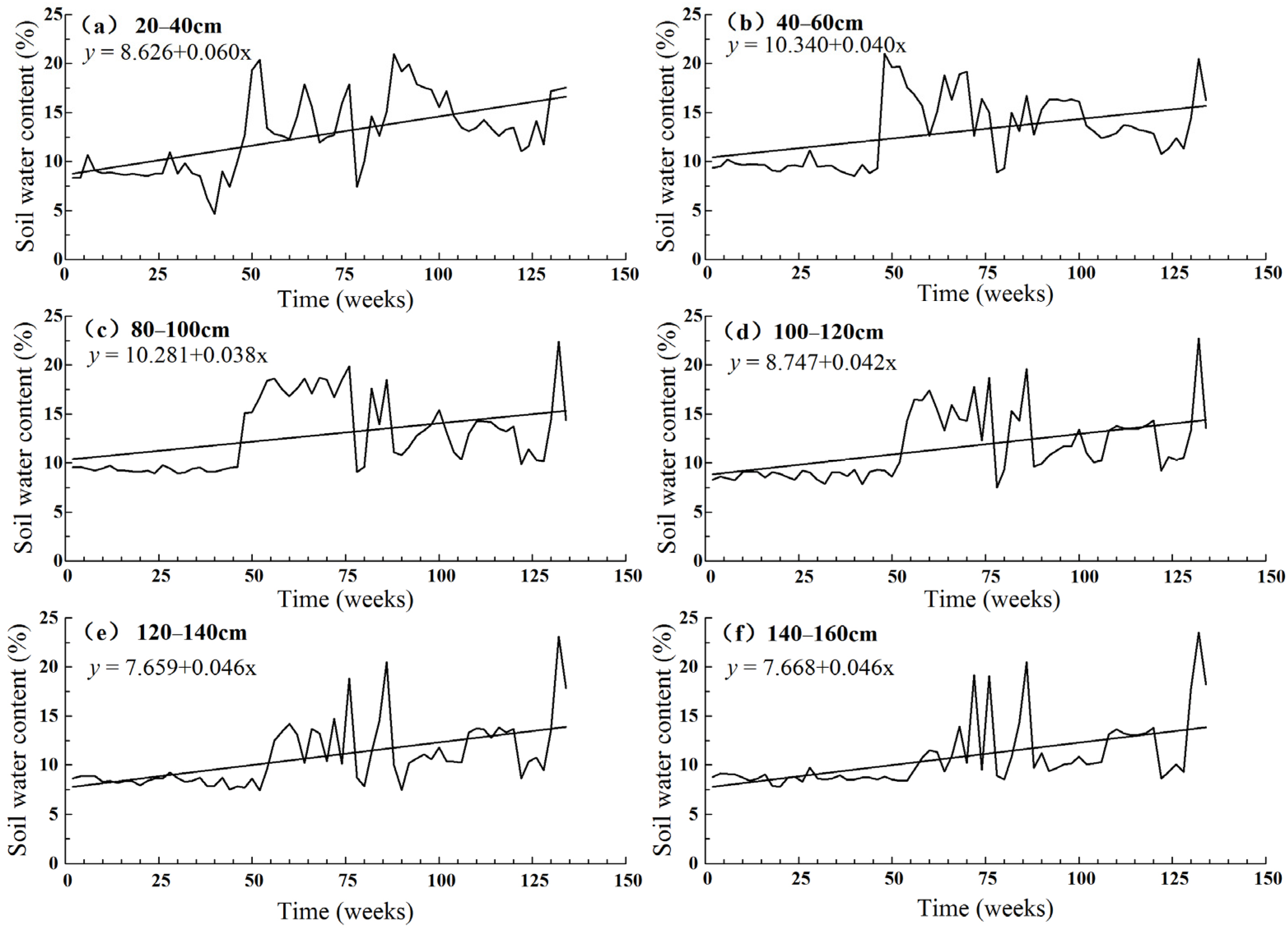
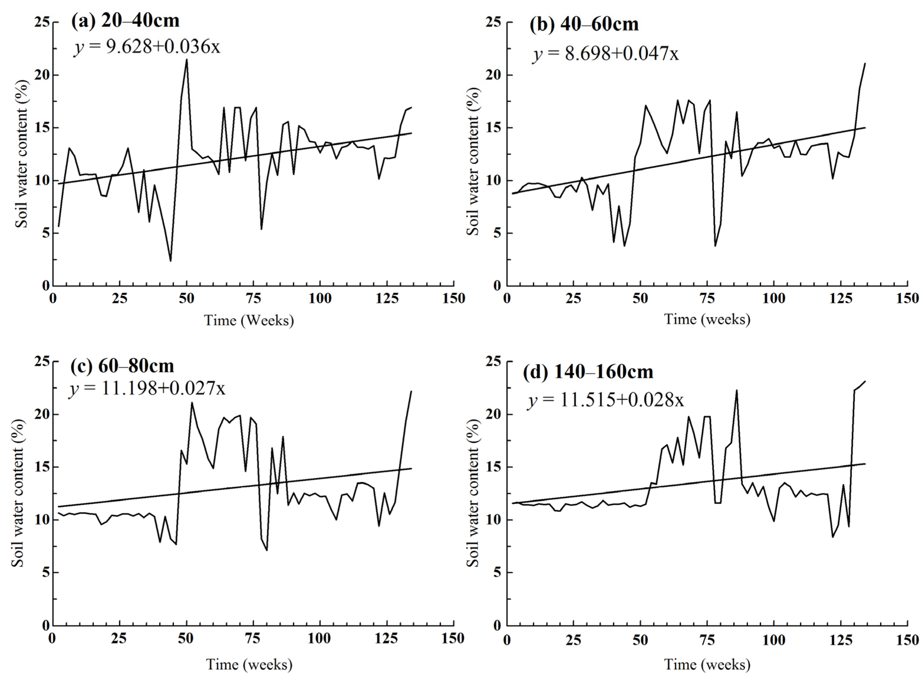
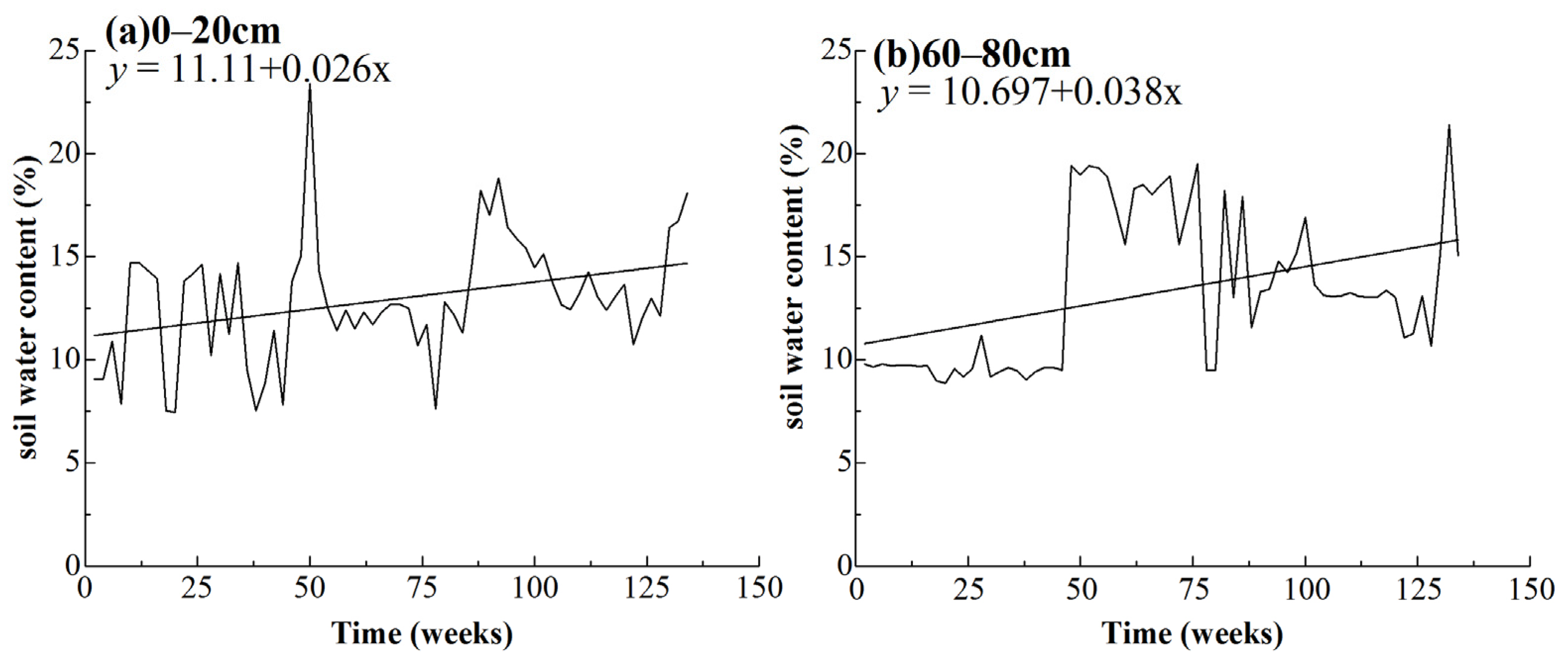
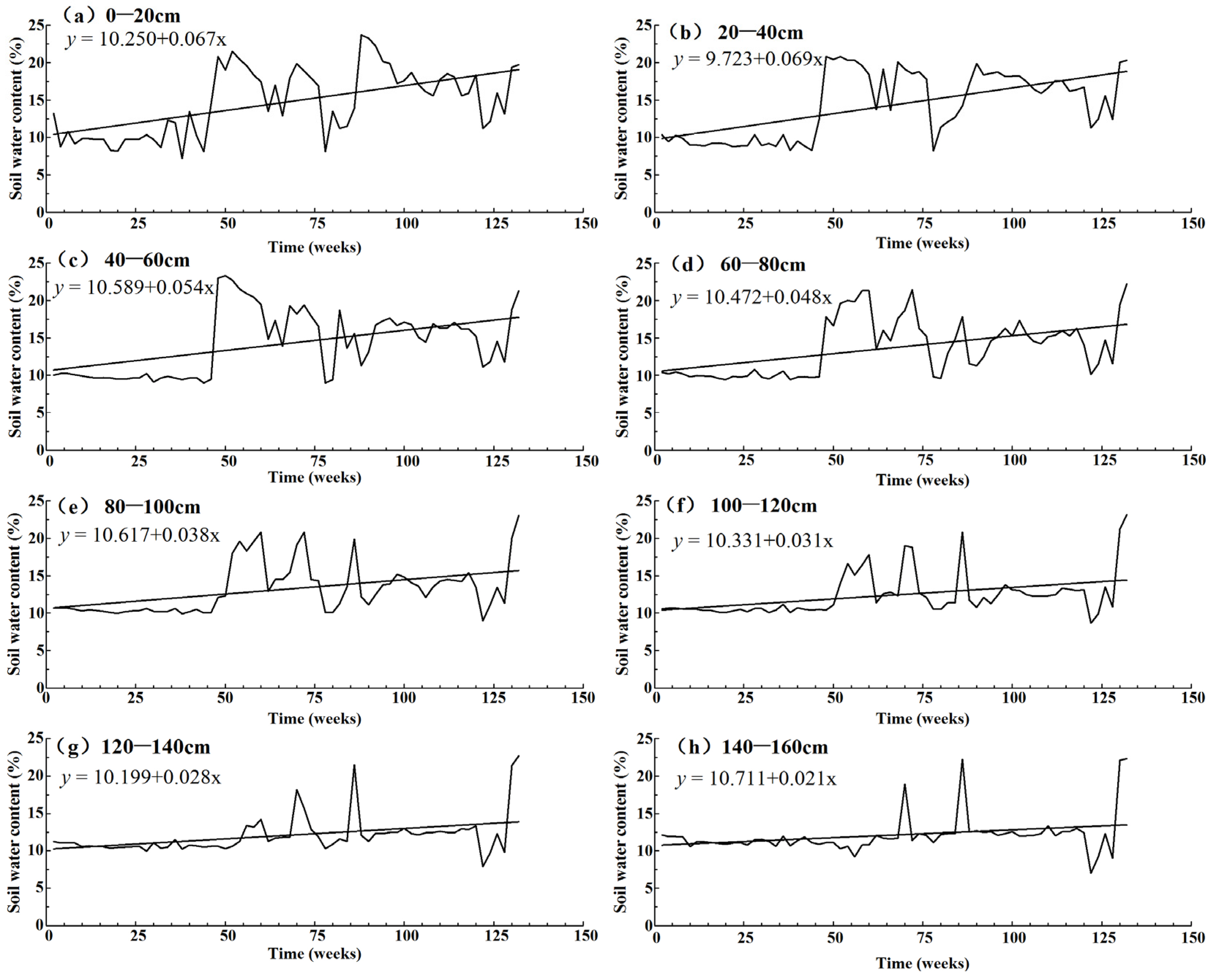
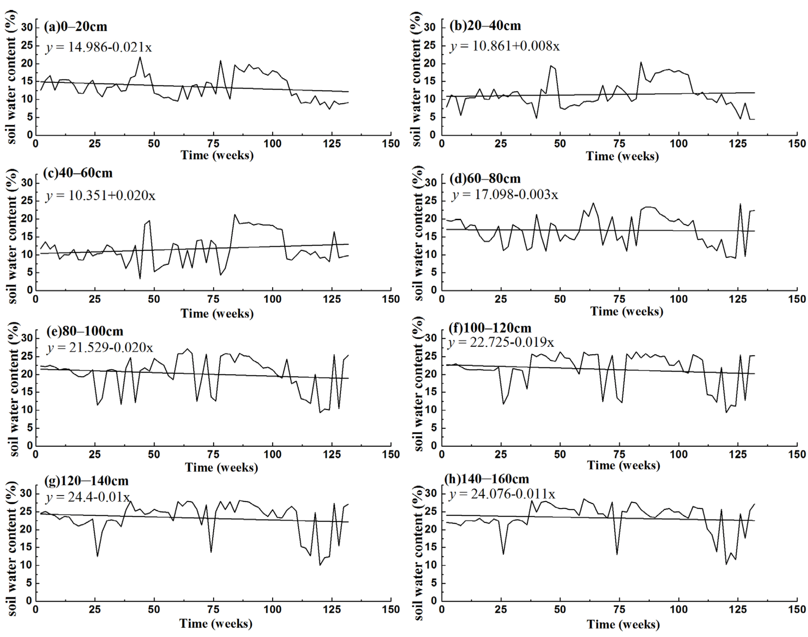
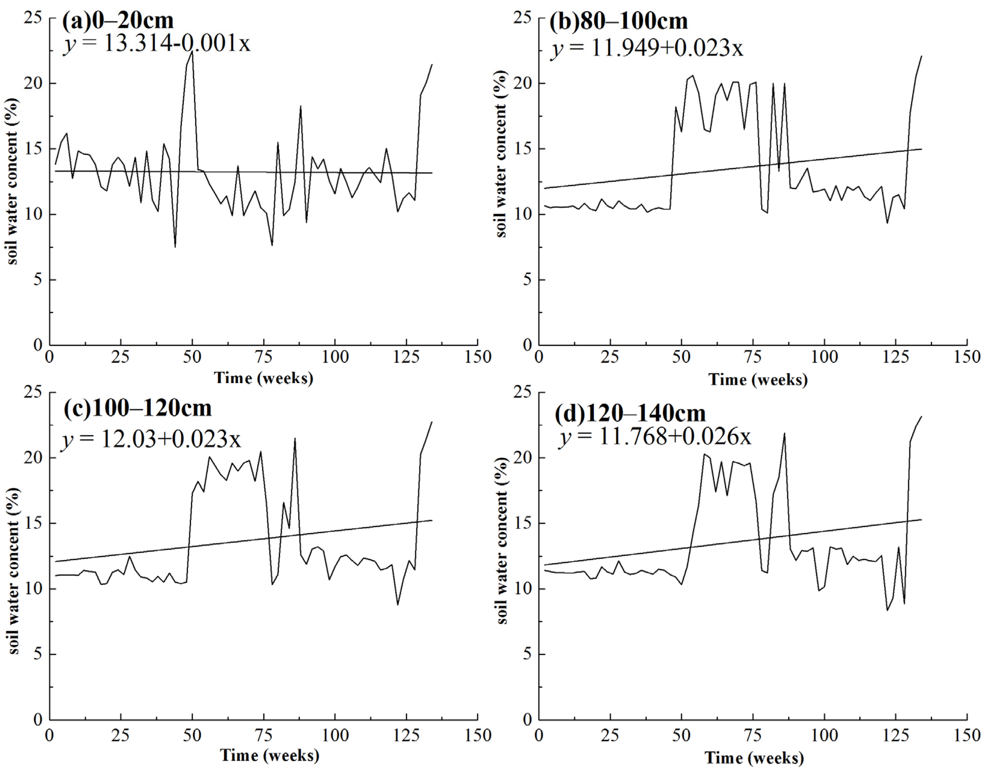
3.2. Trend Analysis of the SWC Series

The M–K test and linear regression were applied to analyze the trends in the SWC of the selected typical vegetation; the results of these tests are presented in

Table 3. Statistical analysis of the SWC trends during the monitoring period.

Vegetation Types	Test	Soil Layer (cm)
		0–20	20–40	40–60	60–80	80–100	100–120	120–140	140–160
Pinus tabulaeformis Carr. plantation	Zs	2.50 *	3.02 **	2.79 **	2.73 **	2.60 **	3.32 **	4.36 **	3.45 **
	b (%/weeks)	0.067	0.069	0.054	0.048	0.038	0.031	0.028	0.021
Prunus sibirica L. plantation	Zs	1.62	2.45 *	2.01 *	1.93	2.04 *	3.27 **	3.05 **	3.65 **
	b (%/weeks)	0.026	0.060	0.040	0.038	0.038	0.042	0.046	0.046
Hippophae rhamnoides Linn. shrub	Zs	−0.23	2.24 *	3.46 **	2.07 *	1.51	1.46	1.82	2.06 *
	b (%/weeks)	−0.001	0.036	0.047	0.027	0.023	0.023	0.026	0.028
Natural grassland	Zs	−1.66	−0.44	0.66	−0.26	−0.31	−0.52	−0.95	−1.17
	b (%/weeks)	−0.021	−0.008	0.020	−0.003	−0.002	−0.019	−0.01	−0.011

Zs: Mann–Kendall (M–K) test; b: slope of linear regression; * statistically significant trends at the 5% significance level; ** statistically significant trends at the 1% significance level.

. For the results that were statistically significant, both the M–K test result (Z_s) and the slope of the linear regression equation (b) for the SWC series of the three types of artificial vegetation were positive, indicating that the SWC series exhibited an increasing tendency during the research period (August 2010–June 2013). For the Pinus tabulaeformis Carr. plantation, a significant increasing trend was observed for the SWC series along the whole research profile; the 0–20 cm soil layer is significant at the 5% level, and the 20–160 cm layer is significant at the 1% level. For the Prunus sibirica L. plantation, the SWC series exhibited a significant increasing tendency (i.e., at the 5% level for the 20–100 cm soil layer and at the 1% level for the 100–160 cm soil layer). For the Hippophae rhamnoides Linn. shrub, the SWC series only increased in the 20–80 cm layer (significant at the 5% level) and the 40–60 cm soil layer (significant at the 1% level). However, in the natural grassland, there was no significant tendency found for the SWC at the whole soil layers. In addition, the coefficients of the regression for the natural grassland are negative for almost of soil layers, which may indicate a decreasing tendency of SWC during the research period.

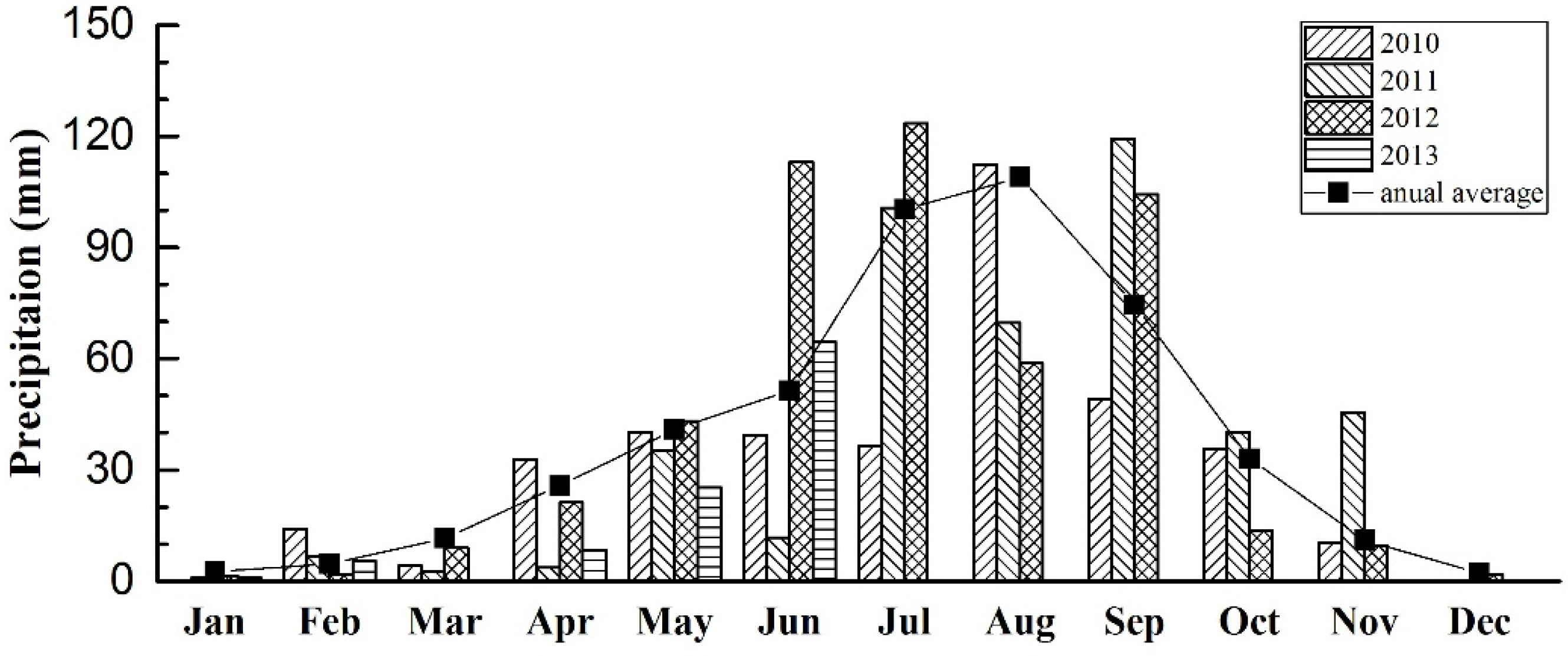
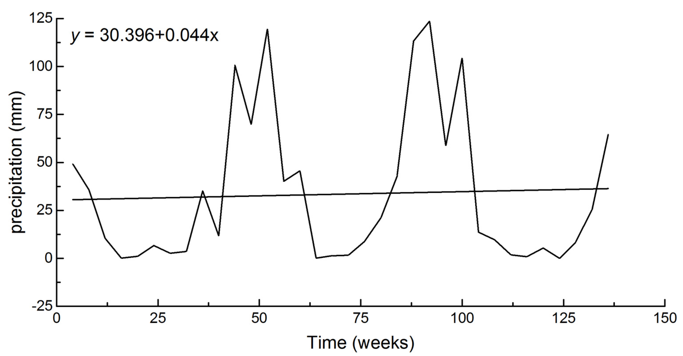
3.3. Trend Analysis of the Precipitation Series

To determine whether the increasing tendency of the SWCs of the three artificial vegetation systems was influenced by precipitation, serial autocorrelation and the PW–MK and M–K trend tests were used to analyze the monthly precipitation series from August 2010 to June 2013. The results show that Z_s = 1.25, and the precipitation series did not exhibit a significant trend during the research period. In addition, Figure 2 shows nonsignificant precipitation increase tendency during the monitoring period. This further verified that the increasing or decreasing trend of the SWC of the artificial vegetation was not caused by precipitation.

3.4. Dynamic Variation Ratio Analysis of SWC Series

The SWC series of the three artificial monovegetation systems that had a significant increasing tendency at the 5% level were chosen to analyze their potential to increase in the 0–160 cm soil layers over the period from August 2010 to June 2013. The results are presented in Figure 3, Figure 4 and Figure 5. Other layers of the plantations and the natural grassland that had no significant variation in SWC during the monitoring period are also shown in Figure 6, Figure 7 and Figure 8.

For the Pinus tabulaeformis Carr. plantation, the SWC had a significant increasing tendency in the 0–160 cm profile, with an increase ratio between 0.021% and 0.069% per week (Figure 3). The results also showed that the SWC increase ratio had an obvious and gradually decreasing tendency as the soil depth changed from 0 to 160 cm. The 20–40 cm layer exhibited the highest increase potential at 0.069% per week compared to only 0.021% for the 140–160 cm layer during the monitoring period.

For the Prunus sibirica L. plantation (Figure 4), a significant increasing tendency in the SWC was also observed over depths of 20–160 cm. The 20–40 cm layer exhibited a higher ratio, 0.060%, and the other layers had a similar ratio of approximately 0.040%. For the artificial shrub Hippophae rhamnoides Linn. (Figure 5), a significant increasing tendency in the SWC occurred in the 20–80 cm and 140–160 cm layers. In addition, the maximum SWC increase ratio was only approximately 0.050% in the 40–60 cm layer compared with 0.030% for the other layers.

As shown in Figure 6, the SWC of the natural grassland has just a slight decreasing tendency in most of the soil layers and without obvious statistical significance. On the other hand, the SWC with nonsignificant trends of Prunus sibirica L. plantation and Hippophae rhamnoides Linn. shrub have a slight increasing tendency in most of the soil layer (Figure 7 and Figure 8).

4. Discussion

Numerous studies focused on the relationship between revegetation and soil water scarcity have suggested that soil water scarcity has become increasingly common in the semiarid regions of China, especially where inappropriate vegetation type, planting density, and land preparation methods have been used. However, the phenomenon of soil water scarcity aggravation did not hold true in the selected research area. During the research period, all the soil water in the revegetation area appeared to exhibit a significant accumulate tendency, while the natural grassland seems to have a slight decreasing trend (without statistical significance).

In the Pinus tabulaeformis Carr. plantation, vegetation construction did not result in soil water loss, and there was a significant tendency for the soil water to accumulate in the 0–160 cm profile. However, previous studies found that the Pinus tabulaeformis Carr. plantation depleted the soil water [14,40]. Chen et al. [14] investigated soil water dynamics without land preparation under Pinus tabulaeformis Carr. plantation and found that pine woodland induced the largest water loss from May to September of 1986–1999 in Dingxi Gansu province, China. Wang et al. [40] studied the depletion depth of different planted vegetation and found that pine forest had depleted deep soil water that accumulated in the previous year; this effect extended to the 21.5 m soil layer in Suide County, Shannxi Province, during late October to early November in 2007. Many factors affect the SWC, such as climate, soil texture, site condition, vegetation density, human activities, and land preparation methods. In our selected area, level bench land preparation method was used, which plays a role in the redistribution of runoff and is beneficial to the SWC. On the other hand, monitoring was usually conducted over several months of a year in previous research, whereas in this paper, the SWC was studied over the entire year, which better reflects the dynamic trend of soil water.

In the Prunus sibirica L. plantation (19 years, 1600 per ha), an accumulation in the SWC was also observed in the 20–60 cm and 80–160 cm layers; the SWCs gradually increased during the monitoring period at ratio of 0.040%–0.060% and 0.038%–0.046% per week, respectively. Nevertheless, other studies showed that soil water scarcity existed under Prunus sibirica L. plantation [41]. Yang et al. [42] investigated the SWC in the 0–2.0 m profile of Prunus sibirica L. plantation (1600 per ha) without land preparation in Dingxi, Gansu Province, China, during late April to early October in 2009. These authors observed that the soil water scarcity phenomenon was particularly severe under the depth of 100 cm. They also stated that the primary reasons for the soil water scarcity may be the unreasonable planting density and vegetation pattern. In our selected plots, the land preparation methods, planting density, climate condition, and soil texture may have had a complex influence on the SWC.

Under the Hippophae rhamnoides Linn. shrub (12 years, 3000 per ha), the SWCs in the 20–80 cm and 140–160 cm layers also showed a significant gradual increasing trend with rates of 0.027%–0.047% per week. However, previous research suggested that soil water was scarce under the Hippophae rhamnoides Linn. shrub [43,44]. Xiao et al. [43] investigated the SWC variability under different land uses during April and October of 2004–2010 in Ansai County, Shaanxi Province, China, and found that SWC decreased annually. Duan et al. [44] measured the SWCs under Hippophae rhamnoides Linn. shrub without any management practices in the Wangdonggou watershed at the Changwu Agro-ecological Experimental Station from April to November in 2013 and May to October in 2014. These authors reported soil water deficits. The difference might due to the effects of the level bench adopted and the planting density, and these results were also confirmed by Cheng [45].

The significant increasing tendency of the SWC was found under the Pinus tabulaeformis Carr. plantation, Prunus sibirica L. plantation and Hippophae rhamnoides Linn. shrub, with the ratios of 0.021%–0.069%, 0.038%–0.06%, and 0.027%–0.047% per week, respectively. Only a slight decreasing tendency in the SWC was found under the natural grassland in 0–160 cm soil layers. The increasing tendency of the Pinus tabulaeformis Carr. plantation was more significant than the other vegetation with respect to extent and amount. This difference was probably caused by different vegetation species and its vertical root distributions characteristics. Studies have found that 50% of the Pinus tabulaeformis Carr. fine roots system is concentrated in the top soil layer (i.e., 0–40 cm [46]); approximately 97% of that is concentrated in the first 0.75 m versus 91% in the first 0.50 m [47]. For Hippophae rhamnoides Linn., the majority of its root system is concentrated in the upper 1.00 m of soil [48,49]. For natural grassland, the majority of its root system is concentrated in the 0–20 cm soil layer [50]. In the Loess Plateau, soil water mainly originates from precipitation. Root systems can improve the soil porosity, create more macropores, and offer access for precipitation infiltration which would be beneficial for soil water content accumulation [2]. These results are consistent with those of previous studies, which reported that forest cover might mitigate drought [20]. The artificial forests/shrub have an obvious canopy structure, and the litter layer and canopy can intercept and collect precipitation [2]. In addition, the litter layer under the artificial forests/shrub can prevent raindrops from directly damaging the soil crust, jamming soil porosity and decreasing the infiltration ratio.

Even though a significant increasing tendency of the SWC was found under the plantation and shrub, and a nonsignificant decreasing tendency found under the natural grassland, the absolute value of SWC in the natural grassland is higher than that of the three kinds of artificial vegetation in some soil layers. To this point, however, it is not reasonable to speculate that the natural grassland is more suitable than the other vegetation types for revegetation in this area. It is because the SWC dynamic processes will reach relative equilibrium values with the progress of population size tending toward stability. Different vegetation types will maintain different equilibrium values due to discrepant root systems, canopy structures, and so on. In the monitoring plots, the population size of three typical artificial monovegetation systems has reached a stable stage and the growth is well. Thus the present SWC condition would meet the water demands of the three kinds of selected artificial vegetation growth, although their SWC keeps a lower level at present.

For the three kinds of artificial vegetation, there is an obvious variation between the first 50 weeks and the subsequent 50 weeks in SWC absolute value for most soil layers. However, the variation was not found under the natural grassland. The obvious variation of the SWC absolute value for the selected artificial vegetation seems to be consistent with the precipitation dynamics during that period. It may indicate that the precipitation amount could influence the SWC absolute value variation of the selected vegetation but have no influence on the SWC dynamic accumulation trend. The difference between the natural grassland and the plantation may come from the different types of root systems and canopy structures.

5. Conclusions

This study systematically investigated the effects of artificial forest/shrub construction on the SWC in 0–160 cm profiles in the Loess Plateau from August 2010 to June 2013. In the study area, the three types of artificial forests/shrub show a soil water accumulation tendency, and the Pinus tabulaeformis Carr. plantation shows the most significant increasing tendency for all of the measured soil layers. At the same time, the natural grassland, used as a contrast group, has no obvious variation in SWC during the monitoring period. This suggests that the phenomenon of soil water accumulation has commonly occurred under the artificial vegetation, such as Pinus tabulaeformis Carr. plantation, Prunus sibirica L. plantation, and Hippophae rhamnoides Linn. Shrub described in this paper.

For the three selected artificial vegetation, the level bench was adopted, but not for the natural grassland. Many factors affect the SWC. Land preparation methods, planting density, and proper species may play an important role in the water accumulation process in this research area. This accumulation phenomenon would benefit plant growth in terms of the sustainable utilization of soil water, as well as soil and water conservation. Therefore, the land preparation methods, plantation species, and its density should be paid much more attention for revegetation in the Loess Plateau.

References

1. Feng, X.M.; Wang, Y.F.; Chen, L.D.; Fu, B.J.; Bai, G.S. Modeling soil erosion and its response to land-use change in hilly catchments of the Chinese Loess Plateau. Geomorphology 2010, 118, 239–248. [Google Scholar] [CrossRef]
2. Zhou, J.; Fu, B.J.; Gao, G.Y.; Lü, Y.H.; Liu, Y.; Lü, N.; Wang, S. Effects of precipitation and restoration vegetation on soil erosion in a semi-arid environment in the Loess Plateau, China. Catena 2016, 137, 1–11. [Google Scholar] [CrossRef]
3. She, D.L.; Zhang, W.J.; Jan, W.H.; Luis, C.T. Area representative soil water content estimations from limited measurements at time-stable locations or depths. J. Hydrol. 2015, 530, 580–590. [Google Scholar] [CrossRef]
4. Gómez-Plaza, A.; Alvarez-Rogel, J.; Albaladejo, J.; Castillo, V.M. Spatial patterns and temporal stability of soil moisture across a range of scales in a semi-arid environment. Hydrol. Processes 2000, 14, 1261–1277. [Google Scholar] [CrossRef]
5. Huang, X.; Shi, Z.H.; Zhu, H.D.; Zhang, H.Y.; Ai, L.; Yin, W. Soil moisture dynamics within soil profiles and associated environmental controls. Catena 2016, 136, 189–196. [Google Scholar] [CrossRef]
6. Pellegrino, A.; Lebon, E.; Voltz, M.; Wery, J. Relationships between plant and soil water status in vine (Vitis vinifera L.). Plant Soil 2004, 266, 129–142. [Google Scholar] [CrossRef]
7. Champagne, C.; Berg, A.A.; McNairn, H.; Drewitt, G.; Huffman, T. Evaluation of soil moisture extremes for agricultural productivity in the Canadian prairies. Agric. For. Meteorol. 2012, 165, 1–11. [Google Scholar] [CrossRef]
8. Wang, S.; Fu, B.J.; Gao, G.Y.; Zhou, J.; Jiao, L.; Liu, J.B. Linking the soil moisture distribution pattern to dynamic processes along slope transects in the Loess Plateau, China. Environ. Monit. Assess. 2015, 187, 778. [Google Scholar] [CrossRef] [PubMed]
9. Liu, Y.X.; Zhao, W.W.; Wang, L.X.; Zhang, X.; Daryanto, S.; Fang, X.N. Spatial variations of soil moisture under Caragana korshinskii Kom. from different precipitation zones: Field based analysis in the Loess Plateau, China. Forests 2016, 7, 31. [Google Scholar] [CrossRef] [Green Version]
10. Wang, Y.Q.; Shao, M.A.; Shao, H.B. A preliminary investigation of the dynamic characteristics of dried soil layers on the Loess Plateau of China. J. Hydrol. 2010, 381, 9–17. [Google Scholar] [CrossRef]
11. Wang, S.; Fu, B.J.; He, C.S.; Sun, G.; Gao, G.Y. A comparative analysis of forest cover and catchment water yield relationships in northern China. For. Ecol. Manag. 2011, 262, 1189–1198. [Google Scholar] [CrossRef]
12. Chen, H.S.; Shao, M.A.; Li, Y.Y. The characteristics of soil water cycle and water balance on steep grassland under natural and simulated rainfall conditions in the Loess Plateau of China. J. Hydrol. 2008, 360, 242–251. [Google Scholar] [CrossRef]
13. Yao, X.L.; Fu, B.J.; Lü, Y.H.; Chang, R.Y.; Wang, S.; Wang, Y.F.; Su, C.H. The multi-scale spatial variance of soil moisture in the semi-arid Loess Plateau of China. J. Soils Sediments 2010, 12, 694–703. [Google Scholar] [CrossRef]
14. Chen, L.D.; Huang, Z.L.; Gong, J.; Fu, B.J.; Huang, Y.L. The effect of land cover/vegetation on soil water dynamic in the hilly area of the loess plateau, China. Catena 2007, 70, 200–208. [Google Scholar] [CrossRef]
15. Liu, B.X.; Shao, M.A. Response of soil water dynamics to precipitation years under different vegetation types on the northern Loess Plateau, China. J. Arid Land 2016, 8, 47–59. [Google Scholar] [CrossRef]
16. Miralles, D.G.; Teuling, A.J.; van Heerwaarden, C.C.; de Arellano, J.V.G. Mega-heatwave temperatures due to combined soil desiccation and atmospheric heat accumulation. Nat. Geosci. 2014, 7, 345–349. [Google Scholar] [CrossRef]
17. Jiao, Q.; Li, R.; Wang, F.; Mu, X.M.; Li, P.F.; An, C.C. Impacts of re-vegetation on surface soil moisture over the Chinese Loess Plateau based on remote sensing datasets. Remote Sens. 2016, 8, 156. [Google Scholar] [CrossRef]
18. Wang, Y.Q.; Shao, M.A.; Zhu, Y.J.; Liu, Z.P. Impacts of land use and plant characteristics on dried soil layers in different climatic regions on the Loess Plateau of China. Agric. For. Meteorol. 2011, 151, 437–448. [Google Scholar] [CrossRef]
19. She, D.L.; Liu, D.D.; Xia, Y.Q.; Shao, M.A. Modeling effects of land use and vegetation density on soil water dynamics: Implications on water resource management. Water Resour. Manag. 2014, 28, 2063–2076. [Google Scholar] [CrossRef]
20. Feng, H.H.; Liu, Y.B. Combined effects of precipitation and air temperature on soil moisture in different land covers in a humid basin. J. Hydrol. 2015, 531, 1129–1140. [Google Scholar] [CrossRef]
21. Luo, Y.; Lei, Z.D.; Zheng, L.; Yang, S.X.; Ouyang, Z.; Zhao, Q.J. A stochastic model of soil water regime in the crop root zone. J. Hydrol. 2007, 335, 89–97. [Google Scholar] [CrossRef]
22. Ford, C.R.; Goranson, C.E.; Mitchell, R.J.; Will, R.E.; Teskey, R.O. Modeling canopy transpiration using time series analysis: A case study illustrating the effect of soil moisture deficit on Pinus taeda. Agric. For. Meteorol. 2005, 130, 163–175. [Google Scholar] [CrossRef]
23. Tarpanelli, A.; Brocca, L.; Lacava, T.; Melone, F.; Moramarco, T.; Faruolo, M.; Pergola, N.; Tramutoli, T. Toward the estimation of river discharge variations using MODIS data in ungauged basins. Remote Sens. Environ. 2013, 136, 47–55. [Google Scholar] [CrossRef]
24. Ghannam, K.; Nakai, T.; Paschalis, A.; Oishi, C.A.; Kotani, A.; Igarashi, Y.; Kumagai, T.; Katul, G.G. Persistence and memory timescales in root-zone soil moisture dynamics. Water Resour. Res. 2016, 52, 1427–1445. [Google Scholar] [CrossRef]
25. Rahmani, A.; Golian, S.; Brocca, L. Multiyear monitoring of soil moisture over Iran through satellite and reanalysis soil moisture products. Int. J. Appl. Earth Obs. Geoinf. 2016, 48, 85–95. [Google Scholar] [CrossRef]
26. Box, G.E.P.; Jenkins, G.M.; Reinsel, G.C.; Ljung, G.M. Time Series Analysis: Forecasting and Control, 5th ed.; Wiley: London, UK, 2015; pp. 2–14. [Google Scholar]
27. Mann, H.B. Nonparametric tests against trend. Econometrica 1945, 13, 245–259. [Google Scholar] [CrossRef]
28. Kendall, M.G. Rank Correlation Methods; Oxford University: Oxford, UK, 1975. [Google Scholar]
29. Barco, J.; Hogue, T.S.; Girotto, M.; Kendall, D.R.; Putti, M. Climate signal propagation in southern California aquifers. Water Resour. Res. 2010, 46, W00F05. [Google Scholar] [CrossRef]
30. Chaudhuri, S.; Dutta, D. Mann–Kendall trend of pollutants, temperature and humidity over an urban station of India with forecast verification using different ARIMA models. Environ. Monit. Assess. 2014, 186, 4719–4742. [Google Scholar] [CrossRef] [PubMed]
31. Kendall, M.; Gibbons, J.D. Rank Correlation Methods, 5th ed.; Oxford University: Oxford, UK, 1990; p. 272. [Google Scholar]
32. Ribeiro, S.; Caineta, J.; Costa, A.C.; Henriques, R.; Soares, A. Detection of inhomogeneities in precipitation time series in Portugal using direct sequential simulation. Atmos. Res. 2016, 171, 147–158. [Google Scholar] [CrossRef]
33. Gado, T.A.; Nguyen, V.T.V. An at-site flood estimation method in the context of nonstationarity II. Statistical analysis of floods in Quebec. J. Hydrol. 2016, 535, 722–736. [Google Scholar] [CrossRef]
34. De Jong, R.; de Bruin, S.; de Wit, A.; Schaepman, M.E.; Dent, D.L. Analysis of monotonic greening and browning trends from global NDVI time-series. Remote Sens. Environ. 2011, 115, 692–702. [Google Scholar] [CrossRef] [Green Version]
35. Sheffield, J.; Wood, E.F. Global trends and variability in soil moisture and drought characteristics, 1950–2000, from observation-driven Simulations of the terrestrial hydrologic cycle. J. Clim. 2008, 21, 432–458. [Google Scholar] [CrossRef]
36. Gao, J.; Williams, M.W.; Fu, X.D.; Wang, G.Q.; Gong, T.L. Spatiotemporal distribution of snow in eastern Tibet and the response to climate change. Remote Sens. Environ. 2012, 121, 1–9. [Google Scholar] [CrossRef]
37. Mediero, L.; Santillan, D.; Garrote, L.; Granados, A. Detection and attribution of trends in magnitude, frequency and timing of floods in Spain. J. Hydrol. 2014, 517, 1072–1088. [Google Scholar] [CrossRef]
38. Zhang, D.W.; Cong, Z.T.; Ni, G.H. Comparison of three Mann-Kendall methods based on the China’s meteorological data. Adv. Water Sci. 2013, 24, 490–496. (In Chinese) [Google Scholar]
39. Zhao, W.J.; Yu, X.Y.; Ma, H.; Zhu, Q.K.; Zhang, Y.; Qin, W.; Ai, N.; Wang, Y. Analysis of precipitation characteristics during 1957–2012 in the semi-arid Loess Plateau, China. PLoS ONE 2015, 10, e0141662. [Google Scholar] [CrossRef] [PubMed]
40. Wang, Z.Q.; Liu, B.Y.; Liu, G.; Zhang, Y.X. Soil water depletion depth by planted vegetation on the Loess Plateau. Sci. China Ser. D Earth Sci. 2009, 52, 835–842. [Google Scholar] [CrossRef]
41. Pérez-Pastor, A.; Ruiz-Sánchez, M.A.C.; Domingo, R. Effects of timing and intensity of deficit irrigation on vegetative and fruit growth of apricot trees. Agric. Water Manag. 2014, 134, 110–118. [Google Scholar] [CrossRef]
42. Lei, Y.; Wei, W.; Baoru, M.; Chen, L.D. Soil water deficit under different artificial vegetation restoration in the semi-arid hilly region of the Loess Plateau. Acta Ecol. Sin. 2011, 31, 3060–3068. (In Chinese) [Google Scholar]
43. Xiao, L.; Xue, S.; Liu, G.B.; Zhang, C. Soil moisture variability under different land uses in the Zhifanggou catchment of the Loess Plateau, China. Arid Land Res. Manag. 2014, 28, 274–290. [Google Scholar] [CrossRef]
44. Duan, L.X.; Huang, M.B.; Zhang, L.D. Differences in hydrological responses for different vegetation types on a steep slope on the Loess Plateau, China. J. Hydrol. 2016, 537, 356–366. [Google Scholar] [CrossRef]
45. Cheng, J.M.; Wan, H.E.; Yong, S.P.; Wang, J. Soil water dynamic of Hippophae rhamnoides in Loess Hilly Region. Acta Bot. Boreal. Occident. Sin. 2003, 23, 1352–1356. (In Chinese) [Google Scholar]
46. Zhang, C.B.; Chen, L.H.; Jiang, J. Vertical root distribution and root cohesion of typical tree species on the Loess Plateau, China. J. Arid Land 2014, 6, 601–611. [Google Scholar] [CrossRef]
47. Ruiz-Sánchez, M.C.; Plana, V.; Ortuño, M.F.; Tapia, L.M.; Abrisquet, J.M. Spatial root distribution of apricot trees in different soil tillage practices. Plant Soil 2005, 272, 211–221. [Google Scholar] [CrossRef]
48. Cong, H.X.; Liang, Y.M.; Li, D.Q. The root system characteristics and soil moisture dynamics of Hippophae rhamnoides in the semi-arid Loess Plateau. Bull. Soil Water Conserv. 1990, 10, 98–103. (In Chinese) [Google Scholar]
49. Liu, C.W.; Du, T.S.; Li, F.S.; Kang, S.Z.; Li, S.; Tong, L. Trunk sap flow characteristics during two growth stages of apple tree and its relationships with affecting factors in an arid region of northwest China. Agric. Water Manag. 2012, 104, 193–202. [Google Scholar] [CrossRef]
50. Wu, C.H.; Chen, Y.M.; Wang, G.L.; Lu, J.L. Vertical distribution characters of typical communities root system in relation to environmental factors in the Hill-gully region of Loess Plateau. Sci. Soil Water Conerv. 2008, 6, 65–70. (In Chinese) [Google Scholar]
Figure 1. Average monthly rainfall of Wuqi County.
Forests 07 00236 g001
Figure 2. The precipitation characteristics for the studied area during the monitoring period.
Forests 07 00236 g002
Figure 3. The SWC increasing ratio for the Pinus tabulaeformis Carr. plantation in different soil layers during the monitoring period.
Forests 07 00236 g003
Figure 4. The SWC increasing ratio for the Prunus sibirica L. plantation in different soil layers during the monitoring period.
Forests 07 00236 g004
Figure 5. The SWC increasing ratio for the shrub Hippophae rhamnoides Linn. in different soil layers during the monitoring period.
Forests 07 00236 g005
Figure 6. The SWC characteristics for the natural grassland in different soil layers during the monitoring period.
Forests 07 00236 g006
Figure 7. The SWC increasing ratio (with no significance trend) for the Prunus sibirica L. plantation in different soil layers during the monitoring period.
Forests 07 00236 g007
Figure 8. The SWC increasing ratio (with no significance trend) for the shrub Hippophae rhamnoides Linn. in different soil layers during the monitoring period.
Forests 07 00236 g008