
Enriching ALS-Derived Area-Based Estimates of Volume through Tree-Level Downscaling


Abstract
:1. Introduction
2. Methods
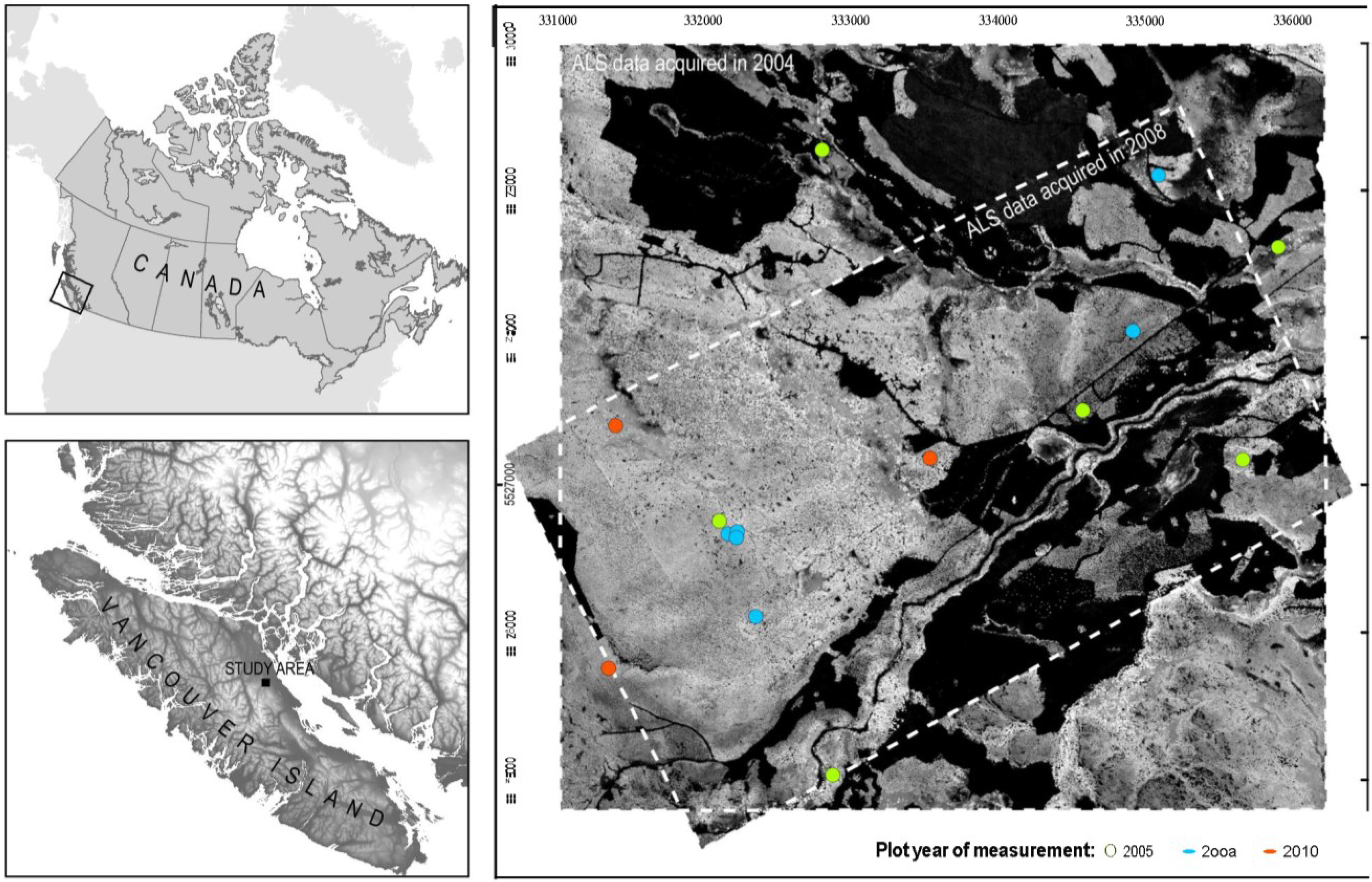
2.1. Study Area

| Study | Study Area | Species Composition | Point Density [points * m−2] | Approach Description | Modelling | Accuracy Assessment |
|---|---|---|---|---|---|---|
| Gobakken and Næsset, 2004 [35] | Norway (6500 ha) | NS, SP | 1 | Weibull parameters estimated with parameter recovery; 24th and 93rd percentile | Linear regression | Based on total plot volume; bias −4.7%–6.6%; SD of differences 11.4%–24.2% |
| Gobakken and Næsset, 2005 [42] | Norway (1000 ha) | NS, SP | 1 | Weibull parameters estimated with parameter recovery; two methods compared: (1) two percentiles and (2) ten percentile system | Linear regression | Based on total plot volume; SD of differences 15.1%–16.4% |
| Maltamo et al., 2007 [37] | Finland (1200 ha) | SP, NS | 0.7 | Parameter prediction; Calibration estimation used to ensure compatibility with plot-level ALS estimates | Maximum likelihood; seemingly unrelated regression | Stem frequency distribution (volume) RMSE: 20.6% |
| Mehtätalo et al., 2007 [41] | Finland (10000 ha) | SP | 0.6 | Parameter recovery based on stand description (volume, height, DBH) | Solution of formulated equation system | Based on total plot volume; bias −0.67%; RMSE 16.7% |
| Packalén and Maltamo, 2008 [43] | Finland (20 km2) | NS, SP; unspec. decid. species | 0.7 ** | Two approaches: (1) nearest neighbor-based predictions; (2) Weibull distribution parameters predicted with k-MSN | k-MSN | Based on DBH distribution; Error index (eP: 0.21–0.34) |
| Thomas et al., 2008 [36] | Ontario, Canada (13,000 km2) | natural hardwood and conifer stands * | (not reported) | Weibull parameters estimated with parameter recovery | Linear regression, finite mixture modelling | R2: 0.65–0.88, RMSE: 0.09–6.05 |
| Peuhkurinen et al., 2008 [47] | Finland (1200 ha) | NS, SP | 0.7 ** | Imputed with kNN | kNN | Based on DBH distribution; Error index (eR: 450.8–605.8) |
| Maltamo et al., 2009 [48] | Norway (960 km2) | NS, SP | 0.7 | Imputed with k-MSN | k-MSN | Based on DBH distribution; Error indices (eR: 75.4–93.2; eP: 0.35–0.39) |
2.2. Plot Selection and Inventory Measurements
| ID | Year of Measurement | Species Percentage | Tree Count | DBH | Height | Total Volume | |||||||
|---|---|---|---|---|---|---|---|---|---|---|---|---|---|
| Fd | Cw | Hw | Dr | Per Plot | Per ha | Mean | SD | Mean | SD | Per Plot | Per ha | ||
| 1 | 2010 | 46.0 | 49.2 | 1.6 | 3.2 | 63 | 700.0 | 21.8 | 9.1 | 22.6 | 6.3 | 29.4 | 421.7 |
| 2 | 2010 | 67.4 | 14.0 | 18.6 | 43 | 477.8 | 27.1 | 6.5 | 27.1 | 5.7 | 30.3 | 465.1 | |
| 3 | 2010 | 12.9 | 87.1 | 31 | 344.4 | 25.0 | 7.3 | 20.0 | 4.4 | 14.3 | 150.4 | ||
| 4 | 2008 | 71.0 | 27.5 | 1.5 | 69 | 766.7 | 29.3 | 10.6 | 27.3 | 8.6 | 62.5 | 974.9 | |
| 5 | 2008 | 76.7 | 16.4 | 6.9 | 73 | 811.1 | 21.6 | 8.0 | 17.9 | 6.3 | 24.0 | 306.5 | |
| 6 | 2008 | 84.3 | 2.0 | 13.7 | 51 | 566.7 | 34.7 | 13.9 | 31.8 | 4.8 | 67.9 | 1018.1 | |
| 7 | 2008 | 81.3 | 15.0 | 3.8 | 80 | 888.9 | 25.7 | 9.2 | 26.1 | 7.9 | 54.7 | 863.0 | |
| 8 | 2008 | 55.8 | 36.4 | 7.8 | 77 | 855.6 | 29.4 | 13.1 | 25.4 | 9.7 | 71.7 | 1079.4 | |
| 9 | 2008 | 86.6 | 8.5 | 4.9 | 82 | 911.1 | 26.5 | 7.7 | 26.4 | 7.3 | 54.7 | 858.5 | |
2.3. ALS Point Clouds
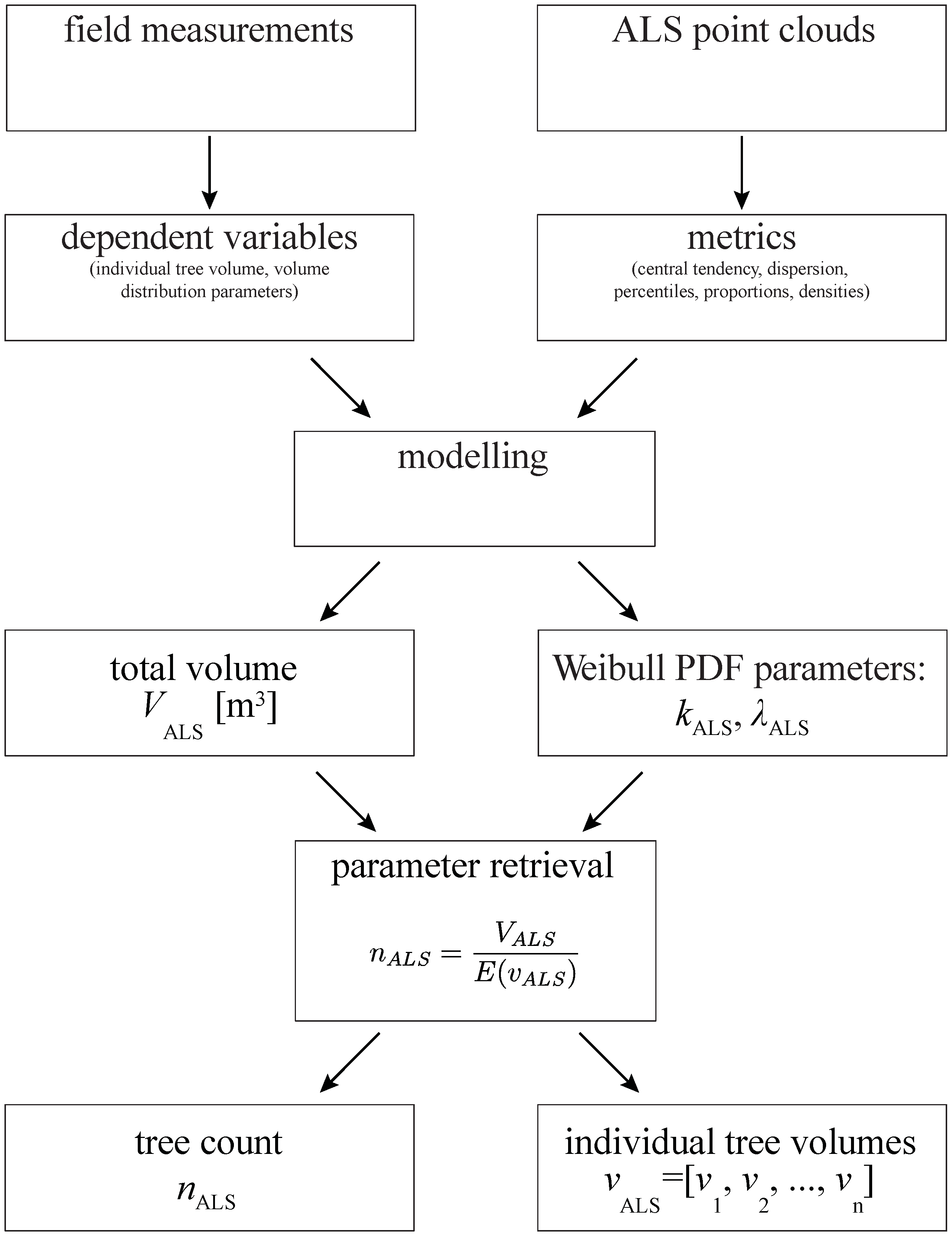
2.4. Modelling Approach

2.5. Modelling Total Plot Volume Using ABA
2.6. Modelling Individual Tree Volume Distribution
2.7. Estimating Tree Count and Individual Tree Volumes
2.8. Validation
3. Results
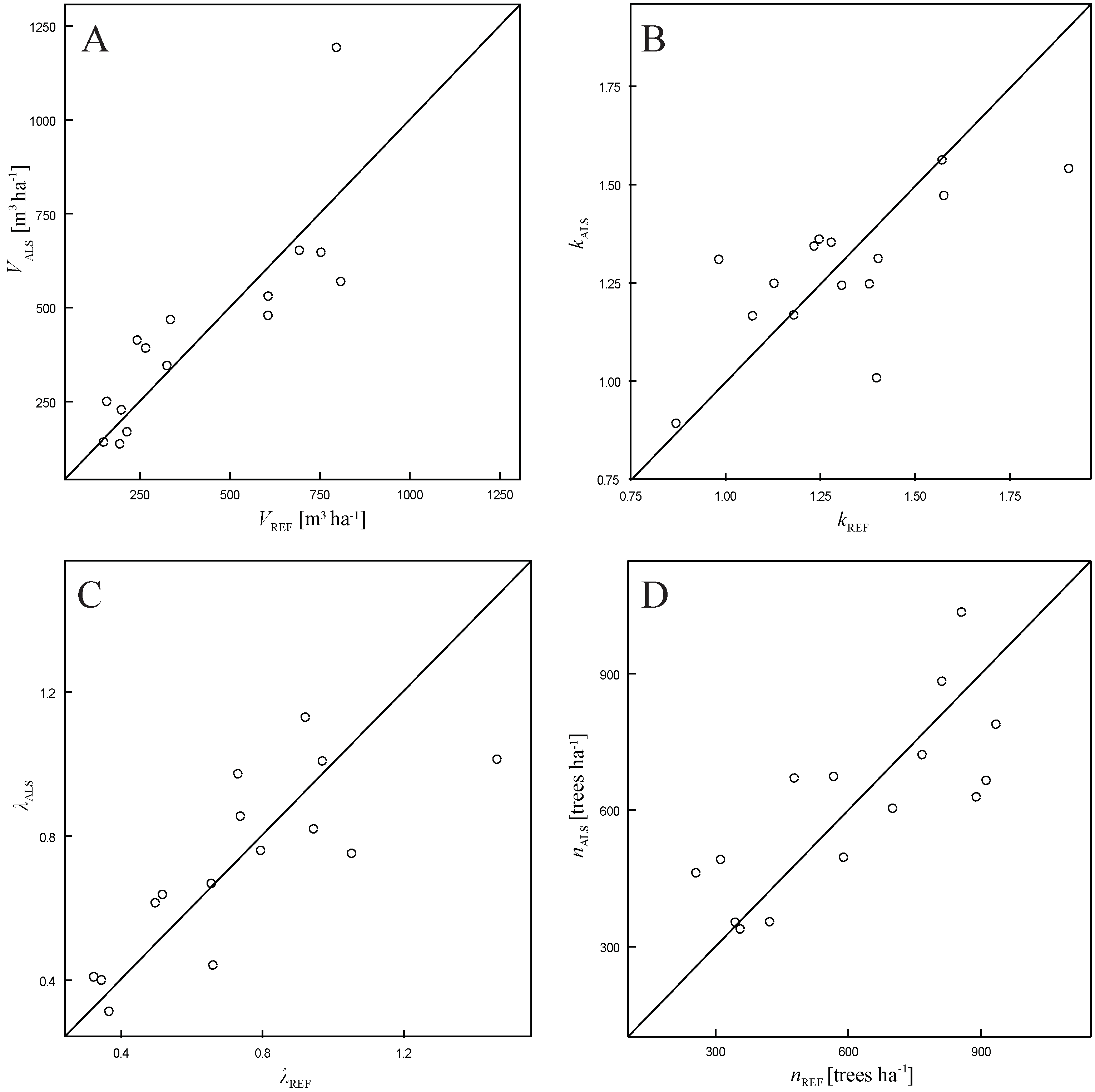
3.1. Total Plot Volume
| Dependent Variable | Predictive Model | R2 (Adjusted) | p-Value |
|---|---|---|---|
| V | 0.867 | 0.00004 | |
| k | 0.562 | 0.00078 | |
| λ | 0.770 | 0.00001 |
| Variable | Bias | Bias% | RMSE | RMSE% | p-Value (Paired Wilcoxon Test) |
|---|---|---|---|---|---|
| V [m3·ha−1] * | 17.2 | 9.55 | 148.0 | 34.8 | 0.89 |
| k * | −0.01 | 0.55 | 0.18 | 13.90 | 0.93 |
| λ * | −0.01 | 2.39 | 0.19 | 25.4 | 0.98 |
| n [trees·ha−1] | −1.60 | 6.81 | 149.5 | 24.4 | 0.97 |

3.2. Weibull Parameters
| Plot Number | Bias | Bias% | RMSE | RMSE% | p-Value (Paired Wilcoxon Test) |
|---|---|---|---|---|---|
| 1 | 0.004 | 92.8 | 0.080 | 91.5 | 0.016 |
| 2 | −0.002 | 216.6 | 0.081 | 408.2 | 0.598 |
| 3 | 0.002 | 768.9 | 0.112 | 1168.3 | 0.038 |
| 4 | 0.005 | −0.5 | 0.039 | 10.5 | 0.146 |
| 5 | 0.013 | −23.7 | 0.068 | 34.3 | 0.598 |
| 6 | 0.011 | −9.8 | 0.106 | 35.4 | 0.700 |
| 7 | 0.005 | 45.9 | 0.109 | 45.0 | 0.047 |
| 8 | 0.020 | 15.4 | 0.114 | 21.6 | 0.006 |
| 9 | 0.000 | 132.5 | 0.064 | 183.1 | 0.416 |
| 10 | −0.024 | 13496.2 | 0.122 | 32599.4 | 0.229 |
| 11 | −0.001 | −14.6 | 0.052 | 18.3 | 0.152 |
| 12 | 0.000 | −28.3 | 0.129 | 41.8 | 0.262 |
| 13 | 0.002 | 80.8 | 0.059 | 76.1 | 0.008 |
| 14 | −0.001 | −48.8 | 0.138 | 44.4 | 0.073 |
| 15 | 0.003 | −13.5 | 0.031 | 19.3 | 0.968 |

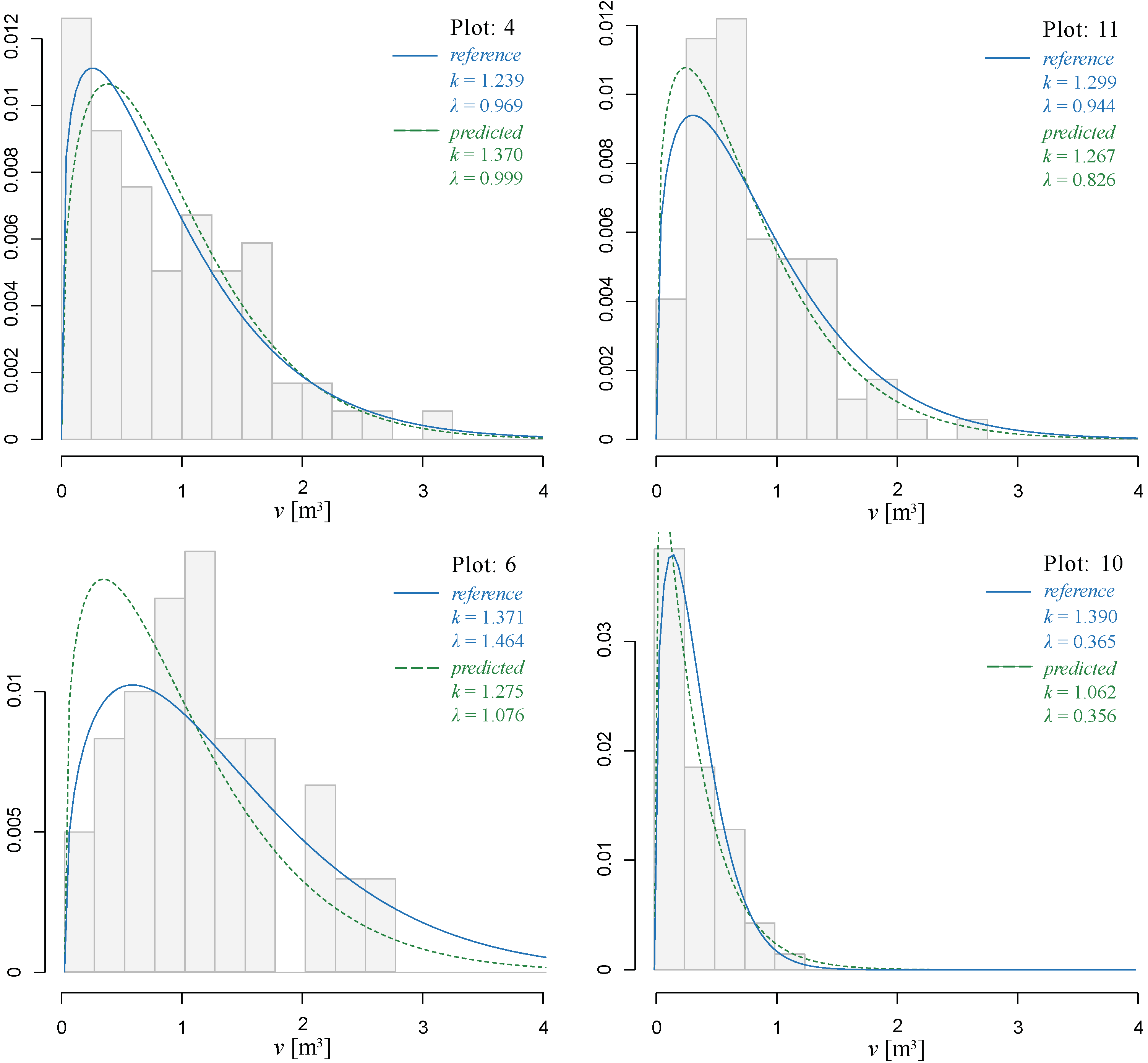
3.3. Individual Tree Volume Frequency Distribution
| Plot Number | eR | eP |
|---|---|---|
| 1 | 62.3 | 0.311 |
| 2 | 72.8 | 0.364 |
| 3 | 53.4 | 0.267 |
| 4 | 83.4 | 0.417 |
| 5 | 43.0 | 0.215 |
| 6 | 76.4 | 0.382 |
| 7 | 102.3 | 0.511 |
| 8 | 131.3 | 0.656 |
| 9 | 82.9 | 0.415 |
| 10 | 71.7 | 0.358 |
| 11 | 55.4 | 0.277 |
| 12 | 65.7 | 0.328 |
| 13 | 58.7 | 0.294 |
| 14 | 66.5 | 0.333 |
| 15 | 49.4 | 0.247 |
| Mean | 71.7 | 0.358 |
4. Discussion
5. Conclusions
Acknowledgements
Author Contributions
Conflicts of Interest
References
- Brosofske, K.D.; Froese, R.E.; Falkowski, M.J.; Banskota, A. A review of methods for mapping and prediction of inventory attributes for operational forest management. For. Sci. 2014, 60, 733–756. [Google Scholar] [CrossRef]
- Corona, P. Integration of forest mapping and inventory to support forest management. IForest 2010, 3, 59–64. [Google Scholar] [CrossRef]
- Brandt, J.P.; Flannigan, M.D.; Maynard, D.G. An introduction to Canada’s boreal zone: Ecosystem processes, health, sustainability, and environmental issues 1. Environ. Rev. 2013, 226, 207–226. [Google Scholar] [CrossRef]
- Watts, S.B.; Tolland, L. Forestry Handbook for British Columbia, 5th ed.; The University of British Columbia: Vancouver, BC, Canada, 2005. [Google Scholar]
- Avery, T.E.; Burkhart, H. Forest Measurements; McGraw-Hill: New York, NY, USA, 2002. [Google Scholar]
- Coops, N.C.; Hilker, T.; Wulder, M.A.; St-Onge, B.; Newnham, G.J.; Siggins, A.; Trofymow, J.A. Estimating canopy structure of Douglas-fir forest stands from discrete-return LiDAR. Trees-Struct. Funct. 2007, 21, 295–310. [Google Scholar] [CrossRef]
- Martinuzzi, S.; Vierling, L.A.; Gould, W.A.; Falkowski, M.J.; Evans, J.S.; Hudak, A.T.; Vierling, K.T. Mapping snags and understory shrubs for a LiDAR-based assessment of wildlife habitat suitability. Remote Sens. Environ. 2009, 113, 2533–2546. [Google Scholar] [CrossRef]
- Andrew, M.E.; Wulder, M.A.; Nelson, T.A. Potential contributions of remote sensing to ecosystem service assessments. Prog. Phys. Geog. 2014, 38, 328–353. [Google Scholar] [CrossRef]
- Froese, R.E.; Shonnard, D.R.; Miller, C.A.; Koers, K.P.; Johnson, D.M. An evaluation of greenhouse gas mitigation options for coal-fired power plants in the US Great Lakes States. Biomass Bioenergy 2010, 34, 251–262. [Google Scholar] [CrossRef]
- Stone, C.; Coops, N.C. Assessment and monitoring of damage from insects in Australian eucalypt forests and commercial plantations. Aust. J. Entomol. 2004, 43, 283–292. [Google Scholar] [CrossRef]
- Wulder, M.A.; Bater, C.C.W.; Coops, N.C.; Hilker, T.; White, J.C. The role of LiDAR in sustainable forest management. For. Chron. 2008, 84, 807–826. [Google Scholar] [CrossRef]
- Lefsky, M.A.; Cohen, W.B.; Acker, S.A.; Parker, G.G.; Spies, T.A.; Harding, D. Lidar remote sensing of the canopy structure and biophysical properties of Douglas-fir western hemlock forests. Remote Sens. Environ. 1999, 70, 339–361. [Google Scholar] [CrossRef]
- Woods, A.J.; Heppner, D.; Kope, H.H.; Burleigh, J.; Maclauchlan, L. Forest health and climate change: A British Columbia perspective. For. Chron. 2010, 86, 412–422. [Google Scholar] [CrossRef]
- White, J.C.; Wulder, M.A.; Buckmaster, G. Validating estimates of merchantable volume from airborne laser scanning (ALS) data using weight scale data. For. Chron. 2014, 90, 378–385. [Google Scholar] [CrossRef]
- Næsset, E.; Bollandsas, O.M.; Gobakken, T.; Bollandsås, O.M. Comparing regression methods in estimation of biophysical properties of forest stands from two different inventories using laser scanner data. Remote Sens. Environ. 2005, 94, 541–553. [Google Scholar] [CrossRef]
- Hudak, A.T.; Haren, A.T.; Crookston, N.L.; Liebermann, R.J.; Ohmann, J.L. Imputing Forest Structure Attributes from Stand Inventory and Remotely Sensed Data in Western Oregon, USA. For. Sci. 2014, 60, 253–269. [Google Scholar] [CrossRef]
- White, J.C.; Wulder, M.A.; Varhola, A.; Vastaranta, M.; Coops, N.C.; Cook, B.D.; Pitt, D.; Woods, M.; Wulder, A.; Cook, D. A best practices guide for generating forest inventory attributes from airborne laser scanning data using an area-based approach. For. Chron. 2013, 89, 722–723. [Google Scholar] [CrossRef]
- Næsset, E.; Økland, T. Estimating tree height and tree crown properties using airborne scanning laser in a boreal nature reserve. Remote Sens. Environ. 2002, 79, 105–115. [Google Scholar] [CrossRef]
- Hyyppä, J.; Inkinen, M. Detecting and estimating attributes for single trees using laser scanner. Photogramm. J. Finl. 1999, 16, 27–42. [Google Scholar]
- Næsset, E. Predicting forest stand characteristics with airborne scanning laser using a practical two-stage procedure and field data. Remote Sens. Environ. 2002, 80, 88–99. [Google Scholar] [CrossRef]
- Breidenbach, J.; Næsset, E.; Lien, V.; Gobakken, T.; Solberg, S. Prediction of species specific forest inventory attributes using a nonparametric semi-individual tree crown approach based on fused airborne laser scanning and multispectral data. Remote Sens. Environ. 2010, 114, 911–924. [Google Scholar] [CrossRef]
- Vastaranta, M.; Holopainen, M.; Yu, X.; Hyyppä, J.; Mäkinen, A.; Rasinmäki, J.; Melkas, T.; Kaartinen, H.; Hyyppä, H. Effects of Individual Tree Detection Error Sources on Forest Management Planning Calculations. Remote Sens. 2011, 3, 1614–1626. [Google Scholar] [CrossRef]
- Vauhkonen, J.; Mehtätalo, L. Matching remotely sensed and field-measured tree size distributions. Can. J. For. Res. 2015, 363, 353–363. [Google Scholar] [CrossRef]
- Reitberger, J.; Schnörr, C.; Krzystek, P.; Stilla, U. 3D segmentation of single trees exploiting full waveform LIDAR data. ISPRS J. Photogramm. Remote Sens. 2009, 64, 561–574. [Google Scholar] [CrossRef]
- Popescu, S.C.; Wynne, R.H. Seeing the trees in the forest: Using lidar and multispectral data fusion with local filtering and variable window size for estimating tree height. Photogramm. Eng. Remote Sens. 2004, 70, 589–604. [Google Scholar] [CrossRef]
- Solberg, S.; Naesset, E.; Bollandsas, O.M. Single tree segmentation using airborne laser scanner data in a structurally heterogeneous spruce forest. Photogramm. Eng. Remote Sens. 2006, 72, 1369–1378. [Google Scholar] [CrossRef]
- Maltamo, M.; Eerikainen, K.; Pitkanen, J.; Hyyppa, J.; Vehmas, M. Estimation of timber volume and stem density based on scanning laser altimetry and expected tree size distribution functions. Remote Sens. Environ. 2004, 90, 319–330. [Google Scholar] [CrossRef]
- Mehtätalo, L.; Virolainen, A.; Tuomela, J.; Packalen, P. Estimating Tree Height Distribution Using Low-Density ALS Data With and Without Training Data. IEEE J. Sel. Top. Appl. Earth Obs. Remote Sens. 2015, 8, 1432–1441. [Google Scholar] [CrossRef]
- Breidenbach, J.; Næsset, E.; Gobakken, T. Improving k-nearest neighbor predictions in forest inventories by combining high and low density airborne laser scanning data. Remote Sens. Environ. 2012, 117, 358–365. [Google Scholar] [CrossRef]
- Wulder, M.A.; Coops, N.C.; Hudak, A.T.; Morsdorf, F.; Nelson, R.; Newnham, G.; Vastaranta, M. Status and prospects for LiDAR remote sensing of forested ecosystems. Can. J. Remote Sens. 2013, 39, 1–5. [Google Scholar] [CrossRef]
- Bergseng, E.; Ørka, H.O.; Næsset, E.; Gobakken, T. Assessing forest inventory information obtained from different inventory approaches and remote sensing data sources. Annals For. Sci. 2014, 72, 33–45. [Google Scholar] [CrossRef]
- Lindberg, E.; Holmgren, J.; Olofsson, K.; Wallerman, J.; Olsson, H. Estimation of tree lists from airborne laser scanning by combining single-tree and area-based methods. Int. J. Remote Sens. 2010, 31, 1175–1192. [Google Scholar] [CrossRef]
- Vastaranta, M.; Kankare, V.; Holopainen, M.; Yu, X.; Hyyppä, J.; Hyyppä, H. Combination of individual tree detection and area-based approach in imputation of forest variables using airborne laser data. ISPRS J. Photogramm. Remote Sens. 2012, 67, 73–79. [Google Scholar] [CrossRef]
- Xu, Q.; Hou, Z.; Maltamo, M.; Tokola, T. Calibration of area based diameter distribution with individual tree based diameter estimates using airborne laser scanning. ISPRS J. Photogramm. Remote Sens. 2014, 93, 65–75. [Google Scholar] [CrossRef]
- Gobakken, T.; Næsset, E. Estimation of diameter and basal area distributions in coniferous forest by means of airborne laser scanner data. Scand. J. For. Res. 2004, 19, 529–542. [Google Scholar] [CrossRef]
- Thomas, V.; Oliver, R.D.; Lim, K.; Woods, M. LiDAR and Weibull modeling of diameter and basal area. For. Chron. 2008, 84, 866–875. [Google Scholar] [CrossRef]
- Maltamo, M.; Suvanto, A.; Packalén, P. Comparison of basal area and stem frequency diameter distribution modelling using airborne laser scanner data and calibration estimation. For. Ecol. Manag. 2007, 247, 26–34. [Google Scholar] [CrossRef]
- Burkhart, H.; Tome, M. Modeling Forest Trees and Stands; Springer: Berlin, Germany, 2012. [Google Scholar]
- Maltamo, M.; Gobakken, T. Predicting Tree Diameter Distributions. In Forestry Applications of Airborne Laser Scanning—Concepts and Case Studies; Maltamo, M., Næsset, E., Vauhkonen, J., Eds.; 2014; pp. 177–191. [Google Scholar]
- Bollandsås, O.M.; Maltamo, M.; Gobakken, T.; Næsset, E. Comparing parametric and non-parametric modelling of diameter distributions on independent data using airborne laser scanning in a boreal conifer forest. Forestry 2013, 86, 493–501. [Google Scholar] [CrossRef]
- Mehtätalo, L.; Maltamo, M.; Packalén, P. Recovering plot-specific diameter distribution and height- diameter curve using als based stand characteristics. In Proceedings of the ISPRS Workshop on Laser Scanning and Silvilaser, Espoo, Finland, 12–14 September 2007; pp. 288–293.
- Gobakken, T.; Næsset, E. Weibull and percentile models for lidar-based estimation of basal area distribution. Scand. J. For. Res. 2005, 20, 490–502. [Google Scholar] [CrossRef]
- Packalén, P.; Maltamo, M. Estimation of species-specific diameter distributions using airborne laser scanning and aerial photographs. Can. J. For. Res. 2008, 38, 1750–1760. [Google Scholar] [CrossRef]
- Humphreys, E.R.; Black, T.A.; Morgenstern, K.; Cai, T.; Drewitt, G.B.; Nesic, Z.; Trofymow, J.A. Carbon dioxide fluxes in coastal Douglas-fir stands at different stages of development after clearcut harvesting. Agric. For. Meteorol. 2006, 140, 6–22. [Google Scholar] [CrossRef]
- Meidinger, D.V.; Pojar, J. Ecosystems of British Columbia; British Columbia: Victoria, BC, Canada, 1991. [Google Scholar]
- Tsui, O.W.; Coops, N.C.; Wulder, M.A.; Marshall, P.L.; Mccardle, A. Using multi-frequency radar and discrete-return LiDAR measurements to estimate above-ground biomass and biomass components in a coastal temperate forest. ISPRS J. Photogramm. Remote Sens. 2012, 69, 121–133. [Google Scholar] [CrossRef]
- Peuhkurinen, J.; Maltamo, M.; Malinen, J. Estimating species-specific diameter distributions and saw log recoveries of boreal forests from airborne laser scanning data and aerial photographs: A distribution-based approach. Silva Fenn. 2008, 42, 625–641. [Google Scholar] [CrossRef]
- Maltamo, M.; Næsset, E.; Bollandsås, O.M.; Gobakken, T.; Packalén, P. Non-parametric prediction of diameter distributions using airborne laser scanner data. Scand. J. For. Res. 2009, 24, 541–553. [Google Scholar] [CrossRef]
- Ung, C.-H.; Bernier, P.; Guo, X.-J. Canadian national biomass equations: New parameter estimates that include British Columbia data. Can. J. For. Res. 2008, 38, 1123–1132. [Google Scholar] [CrossRef]
- Gonzalez, J.S. Wood Density of Canadian Tree Species; Information Report NOR-X-31Forestry Canada; Northwest Region, Northern Forestry Centre: Edmonton, AB, Canada, 1990. [Google Scholar]
- Hilker, T.; Wulder, M.A.; Coops, N.C. Update of forest inventory data with lidar and high spatial resolution satellite imagery. Can. J. Remote Sens. 2008, 34, 5–12. [Google Scholar] [CrossRef]
- Axelsson, P. DEM generation from laser scanner data using adaptive TIN models. Int. Arch. Photogramm. Remote Sens. 2000, 33, 111–118. [Google Scholar]
- McGaughey, R.J. FUSION/LDV: Software for LIDAR Data Analysis and Visualization; US Department of Agriculture, Forest Service, Pacific Northwest Research Station: Seattle, WA, USA, 2014. [Google Scholar]
- R Core Team. R: A Language and Environment for Statistical Computing; R Foundation for Statistical Computing: Vienna, Austria, 2014. [Google Scholar]
- Bouvier, M.; Durrieu, S.; Fournier, R.A.; Renaud, J.-P. Generalizing predictive models of forest inventory attributes using an area-based approach with airborne LiDAR data. Remote Sens. Environ. 2015, 156, 322–334. [Google Scholar] [CrossRef]
- Hollaus, M.; Wagner, W.; Maier, B.; Schadauer, K. Airborne Laser Scanning of Forest Stem Volume in a Mountainous Environment. Sensors 2007, 7, 1559–1577. [Google Scholar] [CrossRef]
- Latifi, H.; Nothdurft, A.; Koch, B. Non-parametric prediction and mapping of standing timber volume and biomass in a temperate forest: Application of multiple optical/LiDAR-derived predictors. Forestry 2010, 83, 395–407. [Google Scholar] [CrossRef]
- Tompalski, P. Wykorzystanie wskaźników przestrzennych 3D w analizach cech roślinności miejskiej na podstawie danych z lotniczego skanowania laserowego. Archi. Fotogram. Kartogr. Teledetekcji 2012, 23, 443–456. [Google Scholar]
- Kane, V.R.; Bakker, J.D.; McGaughey, R.J.; Lutz, J.A.; Gersonde, R.F.; Franklin, J.F. Examining conifer canopy structural complexity across forest ages and elevations with LiDAR data. Can. J. For. Res. 2010, 40, 774–787. [Google Scholar] [CrossRef]
- Kane, V.R.; McGaughey, R.J.; Bakker, J.D.; Gersonde, R.F.; Lutz, J.A.; Franklin, J.F. Comparisons between field- and LiDAR-based measures of stand structural complexity. Can. J. For. Res. 2010, 40, 761–773. [Google Scholar] [CrossRef]
- Means, J.E.; Acker, S.A.; Harding, D.J.; Blair, J.B.; Lefsky, M.A.; Cohen, W.B.; Harmon, M.E.; Mckee, W.A. Use of large-footprint scanning airborne LiDAR to estimate forest stand characteristics in the western Cascades of Oregon. Remote Sens. Environ. 1999, 67, 298–308. [Google Scholar] [CrossRef]
- Sprugel, D. Correcting for bias in log-transformed allometric equations. Ecology 1983, 64, 209–210. [Google Scholar] [CrossRef]
- Westphal, C.; Tremer, N.; von Oheimb, G.; Hansen, J.; von Gadow, K.; Härdtle, W. Is the reverse J-shaped diameter distribution universally applicable in European virgin beech forests? For. Ecol. Manag. 2006, 223, 75–83. [Google Scholar] [CrossRef]
- Bailey, R.L.; Dell, T. Quantifying diameter distributions with the Weibull function. For. Sci. 1973, 19, 97–104. [Google Scholar]
- Delignette-Muller, M.L.; Pouillot, R.; Denis, J.B.; Dutang, C. Fitdistrplus: Help to fit of a parametric distribution to non-censored or censored data. R package version 1.0–3. 2014. Available online: http://cran.r-project.org/web/packages/fitdistrplus/fitdistrplus.pdf (accessed on 1 July 2015).
- Kangas, A.; Maltamo, M. Calibrating predicted diameter distribution. For. Sci. 2000, 46, 390–396. [Google Scholar]
- Deville, J.-C.; Sarndal, C.-E. Calibration Estimators in Survey Sampling. J. Am. Stat. Ass. 1992, 87, 376–382. [Google Scholar] [CrossRef]
- Reynolds, M.R.J.; Burk, T.E.; Huang, W.-C. Goodness-of-FiT tests and Model Selection procedures for diameter distribution models. For. Sci. 1988, 34, 373–399. [Google Scholar]
- Hartigan, J.A.; Hartigan, P.M. The dip test of unimodality. Ann. Stat. 1985, 13, 70–84. [Google Scholar] [CrossRef]
- Kaartinen, H.; Hyyppä, J.; Yu, X.; Vastaranta, M.; Hyyppä, H.; Kukko, A.; Holopainen, M.; Heipke, C.; Hirschmugl, M.; Morsdorf, F.; et al. An international comparison of individual tree detection and extraction using airborne laser scanning. Remote Sens. 2012, 4, 950–974. [Google Scholar] [CrossRef]
- Persson, A.; Holmgren, J.; Söderman, U. Detecting and measuring individual trees using an airborne laser scanner. Photogramm. Eng. Remote Sens. 2002, 68, 925–932. [Google Scholar]
- Van Leeuwen, M.; Nieuwenhuis, M. Retrieval of forest structural parameters using LiDAR remote sensing. Eur. J. For. Res. 2010, 129, 749–770. [Google Scholar] [CrossRef]
- Lindberg, E.; Hollaus, M. Comparison of methods for estimation of stem volume, stem number and basal area from airborne laser scanning data in a hemi-boreal forest. Remote Sens. 2012, 4, 1004–1023. [Google Scholar] [CrossRef]
© 2015 by the authors; licensee MDPI, Basel, Switzerland. This article is an open access article distributed under the terms and conditions of the Creative Commons Attribution license (http://creativecommons.org/licenses/by/4.0/).
Share and Cite
Tompalski, P.; Coops, N.C.; White, J.C.; Wulder, M.A. Enriching ALS-Derived Area-Based Estimates of Volume through Tree-Level Downscaling. Forests 2015, 6, 2608-2630. https://doi.org/10.3390/f6082608
Tompalski P, Coops NC, White JC, Wulder MA. Enriching ALS-Derived Area-Based Estimates of Volume through Tree-Level Downscaling. Forests. 2015; 6(8):2608-2630. https://doi.org/10.3390/f6082608
Chicago/Turabian StyleTompalski, Piotr, Nicholas C. Coops, Joanne C. White, and Michael A. Wulder. 2015. "Enriching ALS-Derived Area-Based Estimates of Volume through Tree-Level Downscaling" Forests 6, no. 8: 2608-2630. https://doi.org/10.3390/f6082608
APA StyleTompalski, P., Coops, N. C., White, J. C., & Wulder, M. A. (2015). Enriching ALS-Derived Area-Based Estimates of Volume through Tree-Level Downscaling. Forests, 6(8), 2608-2630. https://doi.org/10.3390/f6082608