1. Introduction
In order to obtain competitive production costs, large saw mills are often assumed to be required in order to achieve economy-of-scale effects. For instance, the largest saw mills in Sweden had an annual production capacity of more than 400,000 m
3 of sawn wood products, which corresponds to a feed-stock requirement of approximately 800,000 m
3 of timber per year. Put differently, the largest sawmills each demand just under 3% of the total harvested volume of timber in Sweden per year. However, there are a number of challenges for a continued consolidation and expansion of the sawmill industry. For example, the large feed-stock requirements may lead to major logistical challenges. However, the integration of the timber markets also needs to be analyzed and understood in order to make appropriate decisions. According to Goletti
et al. [
1], market integration can be referred to as the co-movement of price, and more generally, to the smooth transmission of price signals and information across spatially separated markets. If the timber markets are integrated, timber is traded across markets and its price fluctuates less, which provides better investment conditions and reduces the need for regional policy decisions.
Regional markets can be said to be integrated if a spatial relationship exists between the regional prices. Studying price relationships between regional timber markets is also important for measuring potential future timber price fluctuations. For instance, since timber sales are the major revenue stream for non-industrial private forest owners, understanding the price fluctuations is of utmost interest to them [
2]. If the regional timber markets are integrated, a price change on one of the markets affects the price on the other markets and will tend to balance the price change across markets. If the market is efficiently integrated, then arbitrage opportunities will, in due course, be exhausted, and the prices will only differ by transaction costs. Contrary to this, with a weak degree of market integration, only an incomplete price transmission occurs. This could occur for a number of reasons, for example, infrastructure restrictions or high transaction costs [
3]. Thus, knowledge about market integration is essential for making appropriate decisions. The degree of market integration will inform the decision-maker on timber trade flows and suitable responses to changing market conditions. In this context, the spatial location of sawmills is also of importance. Not only is the proximity to shipping nodes for the finished products essential, but also the expected spatial impact on the timber markets. For instance, if the relevant timber market is geographically restricted, it is more likely that a local expansion of the sawmill capacity will have a significant effect on the timber price than otherwise. The extreme consequence of this is that capacity investments become uneconomical due to the increasing prices of timber.
The degree to which geographical markets are integrated is best understood by studying the relationship of market prices rather than trade flows. In addition, price can be seen as the best variable to reflect market development because price is a determinant of both demand and supply [
4]. Correlations of price movements have been used in analyses of timber market integration [
5]. A positive and statistically significant correlation coefficient close to one provides support to the hypothesis that two markets are linked. However, this method has been widely criticized for its simple specification and that it may suffer from inferences bias originating from serial correlation, omitted variables, or simultaneity among the prices [
6].
According to the law-of-one-price hypothesis (LOP), arbitrage ensures that timber prices on different markets are similar after necessary adjustments in transaction cost have been made. According to Richardson [
7], the following model can be used to test the LOP:
where
and
denote the prices for commodity
i in time
t in markets 1 and 2, respectively.
represents the transaction costs of trade in commodity
i between the two markets. Estimation is done by transforming Equation (1) into a linear specification using the natural logarithm as follows:
The LOP is evaluated by testing whether the price elasticity,
δ1, is equal to one, while assuming no transaction costs
(i.e.,
δ2 = 0). Consequently, if the LOP holds, the markets are considered to be fully integrated [
8].
However, several problems arise when using Equation (2) to test the LOP. Transaction costs are often unobservable and most of the time, the constant term
δ0 is used as a proxy. Also, if the market prices are determined simultaneously, it will cause endogeneity problems and biased estimates. In general, prices usually tend to follow a random walk. Furthermore, non-stationary properties of prices can also cause regression problems, resulting in a biased LOP test. Another issue is that the possible arbitrage profits may not occur instantly but after several months or years. In this case, the LOP will hold in the long-run rather than in the short-run [
9]. In other words, prices will not drift apart in the long-run and should be co-integrated. The strong form of LOP implies
δ0 = 0 and
δ1 = 1 and the weak form simply removes these restrictions [
10]. The residual term
μit is assumed to be identically and independently distributed. Market integration occurs when a cointegrating relationship is detected among the different timber prices.
The literature on market integration of forest products is quite extensive and summarized in
Table 1. Jung and Doroodian find support for the LOP hypothesis in four regional softwood lumber markets for the period 1950–1985 in the United States [
11]. Baharumshah and Habibullah find evidence of the LOP for Malaysian timber exports of plywood, sawn timber, and wooden moulding
vis-à-vis Singapore, United Kingdom, Germany, United States, Hong Kong, Japan, and Australia using monthly data between January 1985 to December 1992 [
10]. Riis finds evidence of market integration between the Danish and Swedish spruce timber over the period 1954–1992 [
12].
Table 1.
Summary of literature.
Table 1.
Summary of literature.
| Authors | Data/Variables | Main Testing Procedure | Summary of Findings |
|---|
| Jung and Doroodian [11] | Four regional US softwood lumber wood market annual data from 1950 to 1985. | ADF unit root and Johansen cointegration tests. | The LOP is supported. |
| Baharumshah and Habibullah [10] | Monthly data of price of plywood, sawnwood, and wooden moulding for Singapore, UK, Germany, US, Hong Kong, Japan, and Australia from January 1985 to December 1992. | ADF unit root and Engle and Yoo cointegration tests. | The LOP is supported. |
| Riis [12] | Annual data of timber prices over the period 1954–1992 for soft sawnwood for Denmark and Sweden. | ADF unit root and Johansen cointegration tests. | The Swedish and Danish markets are integrated. |
| Hänninen [13] | Quarterly data of import prices over the period 1978–1992 for soft sawnwood for UK, Finland, Sweden, Canada, and Russia. | ADF unit root and Johansen cointegration tests. | The LOP is not supported. |
| Thorsen [14] | Annual data over the period 1951–1991 for sawnwood price for Denmark, Finland, Norway, and Sweden | ADF unit root, Johansen cointegration and causality tests. | The Nordic market is found to be integrated with Finland and Sweden acting as price leaders. |
| Toppinen and Toivonen [15] | Monthly stumpage prices for the period 1958–1996 for roundwood in Finland. | ADF unit root and Johansen cointegration tests. | Markets for stumpage are found to be relatively well integrated. |
| Nanang [16] | Quarterly data over the period 1981–1997 for five regional Canadian softwood lumber markets. | ADF unit root and Johansen cointegration tests. | The LOP is not supported. |
| Toivonen et al. [17] | Annual data over the period 1980–1997 for pine and spruce sawlogs and pulpwood prices for Austria, Finland, and Sweden. | Wald and causality tests. | The Swedish and Finish markets are found to be integrated, with Finland acting as the price-leader. |
| Stevens and Brooks [18] | Quarterly data over the period 1989–1997 for Western hemlock and Sitka spruce logs prices for Alaska, US Pacific Northwest, and Canada. | ADF unit root and Johansen cointegration tests. | Their analysis supports the Western hemlock and Sitka spruce logs from Alaska share an integrated market (Japan) with logs produced in British Columbia and the US Pacific Northwest. |
| Yin and Xu [19] | Monthly data over the period January 1989 to December 1997 for domestic sawlogs, export sawlogs and lumber in the Pacific North-West. | ADF unit root, Johansen cointegration and causality tests. | Two log markets and the two lumber markets are found to be integrated. Yet, the two export log markets are not, nor is any cross-grade combination. |
| Toppinen et al. [20] | Monthly data over the period January 1996 to July 2004 for Estonian, Finnish, and Lithuanian prices of pine, spruce, and birch sawlogs and pulpwood. | ADF unit root and Johansen cointegration tests. | The roundwood markets in the Baltic Sea Area are found to be segmented, with the exception of spruce sawlogs. |
| Shahi et al. [21] | Monthly data over the period 1996–2004 North America. | DF-GLS unit root and Johansen cointegration tests. | The LOP is neither supported in the North American market nor in any combination of one regional market of Canada and all of the five regional markets of the United States, nor in one regional market of the US and all five regional markets of Canada. The regional markets of homogeneous softwood products in the two countries are found to be co-integrated. |
| Tang and Laaksonen-Craig [22] | Monthly data for the period 1988–2004 for five newsprint regional markets in Canada and the US | ADF unit root and Johansen cointegration tests. | The LOP is not supported for regional newsprint markets. For national markets the LOP was valid for the United States but not for Canada. |
| Hänninen et al. [2] | Quarterly data over the period 1995–2003 for sawnwood prices form Austria, the Czech Republic, Estonia, and Finland. | ADF unit root and Johansen cointegration tests. | This European markets tend to be integrated. |
| Mutanen and Toppinen [23] | Quarterly data over the period August 1998–August 2005 for prices of Finnish and Russian spruce sawlogs. | ADF and KPSS unit root and Johansen cointegration tests. | Market integration is not supported. |
| Niquidet and Manley [24] | Monthly price over the period January 1995–December 2006 for log prices in New Zealand. | DF-GLS and KPSS unit root and Johansen and Engle-Granger cointegration tests. | The LOP is supported. |
| Daniels [25] | Quarterly data of stumpage prices from 1984 to 2007 for Western US | ADF unit root and Johansen cointegration tests. | Apart from four regional forests, no evidence supporting the LOP is uncovered for national forest timber markets |
Hänninen tests the LOP for imports of soft sawn wood to the United Kingdom from Finland, Sweden, Canada, and Russia [
13]. The results do not support the LOP. Thorsen concludes that the coniferous timber markets in Denmark, Finland, Norway, and Sweden are integrated, with Sweden and Finland as price-leaders [
14]. Toppinen and Toivonen analyze the integration of roundwood markets in Finland using monthly stumpage prices for the period 1958–1996 and conclude that the markets are integrated [
15].
Nanang tests the LOP for five regional softwood markets in Canada (Atlantic Canada, Quebec, Ontario, Prairies, and British Columbia) using quarterly data for the period 1981–1997 [
16]. They reject the LOP hypothesis, implying that no single market for softwood exists. Toivonen
et al. examine roundwood markets in Austria, Finland, and Sweden by using annual delivery prices of pine and spruce sawlogs and pulpwood from 1980 to 1997 [
17]. The Swedish and Finish markets are found to be integrated, with Finland as price-leader, whilst the Austrian market is not.
Stevens and Brooks test whether the markets for Alaskan lumber and logs are integrated with those of similar products from the US Pacific Northwest and Canada [
18]. They use quarterly data over the period 1989 to 1997 and conclude that the Alaskan market for spruce logs is integrated with the log markets in British Columbia and the US Pacific Northwest. However, the lumber markets are not integrated. Yin and Xu study six sawlogs and lumber markets in the Pacific Northwest using monthly data over the period January 1989 to December 1997 and find evidence of integrated markets [
19]. Toppinen
et al. analyze the development of Estonian, Finnish and Lithuanian roundwood markets using nominal monthly time series of delivery prices of pine, spruce and birch sawlogs and pulpwood for the period January 1996 to July 2004 [
20]. Overall, the roundwood markets are found to be segmented with the exception of spruce sawlogs.
Shahi
et al. explore the existence of the LOP in North American markets (10 regions) for aggregate softwood lumber and homogeneous softwood lumber products [
21]. For this purpose, they make use of monthly price data for the period 1996–2004. They conclude that the LOP hypothesis can be rejected for aggregate softwood lumber markets, both in the North American market as well as in any combination of one regional market of Canada, all of the five regional markets of the United States, and in one regional market of the United States and all five regional markets of Canada. However, the regional markets of homogeneous softwood products are found to be co-integrated.
Tang and Laaksonen-Craig test the LOP for five Canadian and US regional markets of newsprint (British Columbia, Ontario, Quebec, US East, and US West) using monthly data for 1988–2004 [
22]. They reject the LOP hypothesis for the regional markets and the national Canadian market while the hypothesis could not be rejected for the national US market. Hänninen
et al. study the forest markets in Austria, the Czech Republic, Estonia, and Finland to determine the degree of market integration between old and new European Union countries [
2]. Their results suggest a gradual integration of the European forest markets. Mutanen and Toppinen examine the price dynamics in roundwood exports from Russia to Finland for sawlog and pulpwood prices over the quarterly period August 1998 to August 2005 [
23]. According to the cointegration tests, the prices of Finnish and Russian spruce sawlogs have moved closely together. The price changes of spruce sawlogs in the Finnish roundwood market are reflected in the Russian prices, but not
vice versa. Price co-movement and consequent market integration was not detected. Niquidet and Manley examine the integration of log prices in New Zealand using monthly price from January 1995 to December 2006 [
24]. Prices for exports display significant integration across regions and generally follow the LOP. Daniels studies market integration for 62 national forests in the Western US by using quarterly stumpage prices from 1984 to 2007 [
25]. Prices from only four regions are found to be linked and can thus be modeled as integrated stumpage markets. Aside from these four forests, the LOP hypotheses are rejected for national forest timber markets in the Western US.
As shown in
Table 1, several studies on market integration have been done for Sweden but in relation to other countries. The purpose of this paper is to add further empirical evidence to this literature by assessing the degree of market integration for timber markets within Sweden. The extent to which the markets are integrated is a vital indicator of efficiency and performance of its pricing.
2. Method and Materials
Unit root and co-integration tests are usually performed to appraise whether the regional prices follow a common or separate stochastic trend in the long-run. Unit root can be described as a feature of the underlying processes affecting the price level, which evolves through time. This process can either be stationary or non-stationary, that is, deviations from the long-term trend are either stationary or non-stationary. If timber price is found to be non-stationary, then the price effect from market shocks will tend to be persistent. That is, the timber price will not return to its previously long-run trend; instead, a new trend is established. On the contrary, if timber price is found to be stationary, then the price effect from the market shock is temporary and the price for timber will eventually return to its long-term level.
Evidence of a common trend lends support to the LOP hypothesis. To this end, a vector error-correction mechanism (VECM)-based causality test is conducted to identify whether a specific region is acting as a price-leader, transmitting its price across the other timber markets. Finally, variance decompositions and impulse response functions are employed to assess the dynamic properties of the timber markets. Conventional augmented Dickey-Fuller (ADF) unit root test, as developed by Dickey and Fuller [
26], are first computed. The ADF tests the null hypothesis (H
0) of non-stationarity and can be supplemented with a test of the H
0 of stationarity, such as the KPSS test (Kwaitkowski, Phillips, Schmidt and Shin test) [
27]. The joint testing is commonly known as confirmatory analysis [
28]. But when data of higher frequency, such as monthly or quarterly, are used, the spurious regression problem may arise due to seasonality in the series [
29]. Hylleberg
et al., [
30] recommend their own HEGY test (Hylleberg, Engle, Granger and Yoo test) which allows for the simultaneous testing for a unit root at frequency zero
; that is, a non-seasonal unit root when a unit root may be present at some or all of the seasonal frequencies.
The ADF, KPSS, and HEGY tests ignore the occurrence of structural breaks in the data, and this can result in reduced explanatory power of the tests to reject a unit root, even in the presence of a trend of stationarity [
31]. Breaks are usually associated with anomalous events and can occur due to economic, political, or climatic shocks. Phillips and Perron are amongst the firsts to account for a break when testing for a unit root in time-series [
32]. However, their test tends to suffer similar shortcomings to the ADF test and also makes use of an exogenous or known break. As indicated by Christiano [
33], such a feature can cause the invalidation of the sampling distribution theory underlying conventional time-series unit root tests. Zivot and Andrews recommend a test that allows for one break to be endogenously determined by the time-series [
34]. However, in the presence of two or more breaks, the Zivot-Andrews test tends to lose power. Narayan and Popp suggest a test which allows for the presence of two endogenous breaks [
35]. Their test is argued to have correct size, stable power, and is able to identify structural breaks accurately. Thus, their test will mainly be considered. Apart from Andersson [
36] and a few others, most of the studies done in relation to forest product prices have ignored the impact of breaks.
Two specifications are considered when testing for a unit root. One specification applies a regression which includes a constant term only, while the other contains both a constant term and a time trend. Since time-series data tend to exhibit a trend over time, it is more appropriate to consider a regression with both a constant term and a trend. First differencing is likely to remove any deterministic trends. In that case, the regression should include a constant only. For the sake of comparison, both specifications are estimated, underlying the importance of performing appropriate tests. Let a time-series variable, Pt, be integrated by the order of d; That is, Pt~I(d). If the variable is I(0), then it is said to be stationary. In general, time-series data tends to be non-stationary and I(1).
Series must be integrated of the same order to study a cointegrating relationship. Similar to unit root test, a cointegration test also tends to suffer from the presence of a structural break. Gregory and Hansen advocate an ADF co-integration test, which accounts for a break [
37]. The H
0 of no co-integration with a structural break is tested against the alternative hypothesis (H
1) of the existence of one break.
An integrated market should exhibit causal linkages among prices. Indeed, cointegration implies causality in at least one direction [
38]. The leader–follower connection is of particular interest when evaluating market integration. Granger causality test allows us to evaluate which market is leading others in terms of price adjustment. The VECM-based Granger-causality test, which makes use of the first-differenced stationary data, will be employed. The essence of the VECM lies in the use of co-integrated series to avoid the problem of spurious regressions. The
ρth order of the VECM structure can be represented as in the following equation:
where
t = 1, 2, …,
T,
and
are parameters to be estimated.
ECMt−1 represents the one period lagged error-term derived from the cointegrating vector, and the error terms
ε1,
ε2, and
ε3 are serially independent with a mean of zero and finite covariance matrix. The
LPN,
LPM, and
LPS are the timber prices for the three regional markets investigated. The coefficients on the
ECM represent how fast deviations from the long-run equilibrium are eliminated. Given the use of a VAR structure, all variables are treated as endogenous variables.
The VECM model is augmented by a dummy variable
D which is defined as:
where
b denotes the point at which the break occurs.
D captures any structural shocks arising at a given point in time,
t. The break dates are obtained from the Narayan-Popp time-series unit root tests of two breaks in the level and slope of a trending series for the
LPN,
LPS, and
LPM series. These dates are used to construct a proxy for the shocks. While the dummy variable controls for any shifts in the dependent variable, it also provides a means to minimize misspecification bias.
A Wald test for the joint significance can be exploited to examine the direction of any causal relationship among the variables. For instance, LPM does not Granger-cause LPN if and only if all the coefficients β12,1k; are not significantly different from zero in Equation (3). That is, the dependent variable reacts only to short-term shocks. This can be referred to as the short-run Granger causality test. Long-run causality can be investigated via a weak exogeneity test by testing for H0: = 0. This test can be referred to as the long-run Granger causality test. The statistical significance of the lagged error-correction term can be measured by applying separate t-tests on the adjustment coefficients. If the null is not rejected, then LPM and LPS do not Granger-cause LPN in the long-run. Moreover, it is necessary to check whether the two sources of causation are significant. For instance, if all the coefficients β12,1k; and are jointly not significantly different from zero, then LPM does not strongly Granger-cause LPN in the long-run. This test can be referred to as the strong Granger causality test. If no causality is found, then the neutrality hypothesis holds.
The goodness-of-fit of the VECM is based on the
R2. Conventional diagnostic tests include the omitted-variable bias regression equation specification error test (RESET) of DeBenedictis and Giles [
39], the Jarque and Bera normality test [
40], the Breusch and Pagan heteroskedasticity test [
41], and the Breush and Godfrey serial correlation test [
42,
43]. A variance inflation factor (VIF) of 5 or 10 indicates a multicollinearity problem [
44].
The VECM-based Granger causality test only indicates whether or not the dependent variable is exogenous. It does not provide any information about the dynamic properties of the system of equations and relative strength of a variable beyond the sample period. These properties can be indicated by computing the forecast error variance decompositions and impulse response functions. They can allow an examination of the short-run and long-run dynamics among the economic variables and inferences about the direction of causal flows among the variables. Variance decomposition refers to the breakdown of the change in value of a variable in a given period arising from its own shocks and shocks in other variables. To some extent, the quantification of any causal relationship can be fashioned through variance decompositions [
45].
Impulse response functions trace any persistent or transient temporal responses of a shock in one market as well as in other markets. If a shock dies out quickly and the impulse responses converge after a quarter or two, then the markets can be considered highly integrated but also highly independent from of each other. However, if the shocks accumulate over time, then the markets can be considered as interdependent. The two approaches are based on the Cholesky decomposition method to orthogonalize the exogenous shocks [
46].
Nominal quarterly delivery price data of spruce and pine timber for three regions over the period 1999Q1 to 2012Q4 are obtained from the Swedish Forest Agency [
47].Price data for the third quarter 2002 was not available for Northern Sweden. Consequently, price for the third quarter of 2002 was calculated by interpolating the prices for the second quarter of 2002 and the final quarter of 2002. According to the Timber Measurement Associations [
48], a total of 76.6 million m
3 (solid volume excluding bark) of roundwood was harvested in 2012, of which 32% came from the Northern region, 43.2% from the central region, and 24.8% from the Southern region. A brief description of the data is presented in
Table 1.
LPN,
LPM, and
LPS denote the natural logarithm of the real delivery prices of spruce and pine timber (in Swedish Krona, SEK) in the Northern, central, and Southern region, respectively. Quarterly producer price index data is used to compute the real prices.
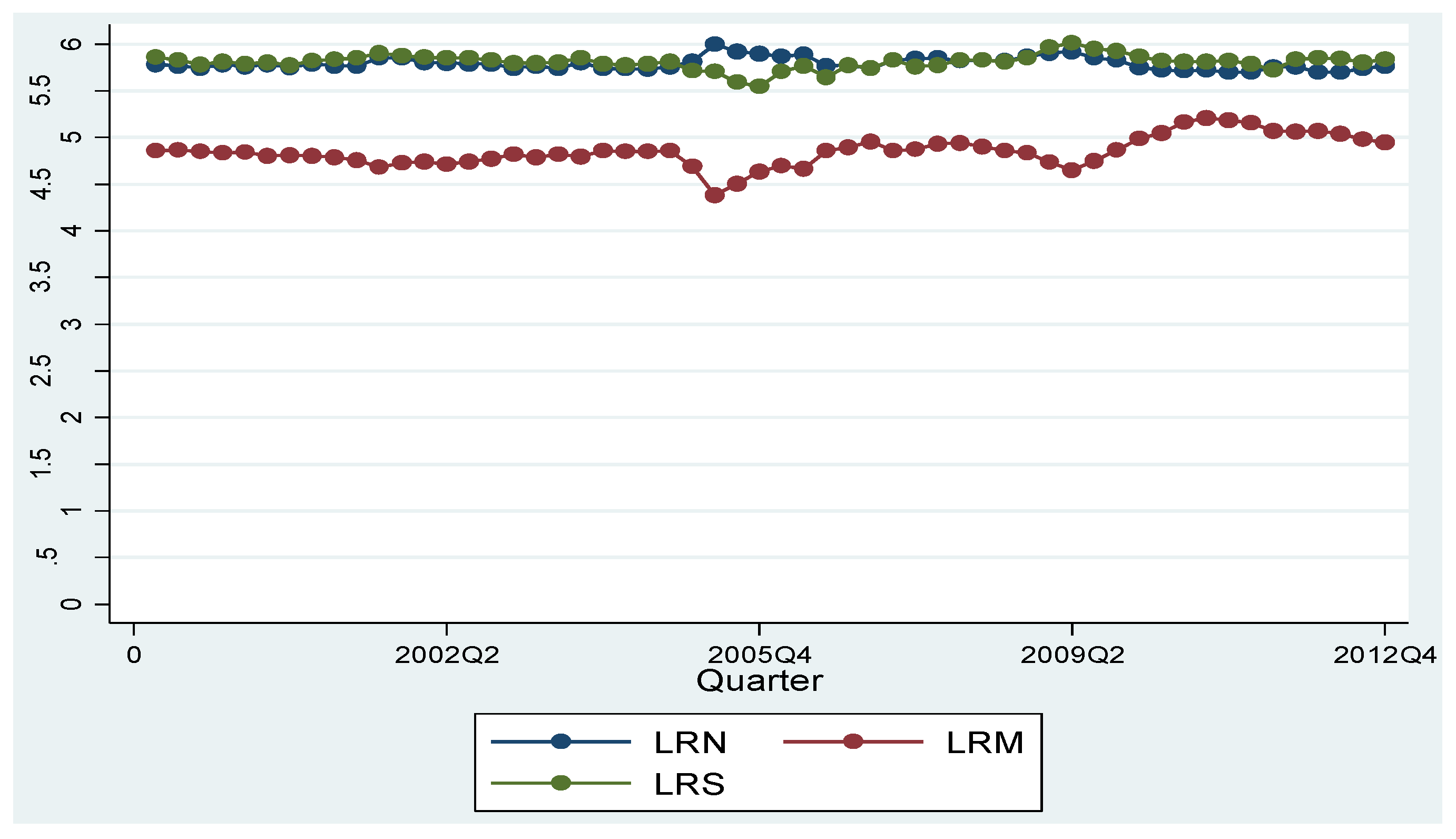
Figure 1 shows the trend of each variable over the time period.
Figure 1.
Prices of Spruce and Pine Sawlogs Trends. LPN, LPM, and LPS denote the natural logarithm of the real delivery prices of spruce and pine timber (in Swedish Krona, SEK) in the Northern, central, and Southern region, respectively.
Figure 1.
Prices of Spruce and Pine Sawlogs Trends. LPN, LPM, and LPS denote the natural logarithm of the real delivery prices of spruce and pine timber (in Swedish Krona, SEK) in the Northern, central, and Southern region, respectively.
When markets are poorly integrated, prices tend to be highly volatile. The degree of price volatility is measured by the standard deviation in
Table 2. The prices in the three regions tend to be moderately volatile, especially in the Northern and Southern regions.
Table 2.
Descriptive statistics of spruce and pine sawlogs.
Table 2.
Descriptive statistics of spruce and pine sawlogs.
| Series | Mean | Standard Deviation | Minimum | Maximum |
|---|
| LPN | 5.793 | 0.064 | 5.696 | 5.994 |
| LPM | 4.851 | 0.159 | 4.383 | 5.211 |
| LPS | 5.810 | 0.078 | 5.549 | 6.010 |
3. Results
Preliminary results can be obtained by investigating the degree of correlation among the timber prices.
Table 3 reports the pairwise correlation coefficients. Only the correlation between
LPN and
LPM is found to be statistically significant.
The maximum lag length (
kmax) for all unit root and co-integration tests is chosen according to the Bartlett kernel, that is, 4(
T/100)
2/9 where
T = 56. Since the metric is computed to less than four,
kmax is set to three. Following the discussion above on the order of integration of a time-series, the ADF tests reveal an I(1) process for the
LPN and
LPS series, while
LPM is found to be stationary. However, the KPSS tests confirm a non-stationary and I(1) process for all three price series. The ADF and KPSS statistics are reported in
Table 4.
Table 3.
Pairwise correlation matrix.
Table 3.
Pairwise correlation matrix.
| Series | LPN | LPM | LPS |
|---|
| LPN | 1.000 | - | - |
| | | |
| LPM | −0.780 | 1.000 | - |
| (0.000) * | | |
| LPS | −0.059 | 0.159 | 1.000 |
| (0.667) | (0.242) | |
Table 4.
Time series unit root tests without break.
Table 4.
Time series unit root tests without break.
| Series | ADF | KPSS |
|---|
| Level Form | First Difference | Level Form | First Difference |
|---|
| Without Trend | With Trend | Without Trend | With Trend | Without Trend | With Trend | Without Trend | With Trend |
|---|
| LPN | −2.806(0) ‡ | −2.842(0) | −7.673(0) * | −7.610(0) * | 0.220(2) | 0.210(2) + | 0.043(3) | 0.037(3) |
| LPM | −2.429(1) | −3.219(1) ‡ | −5.318(0) * | −5.268(0) * | 0.847(2) * | 0.216(2) + | 0.054(2) | 0.042(2) |
| LPS | −2.686(0) ‡ | −2.690(0) | −8.180(0) * | −8.096(0) * | 0.210(2) | 0.190(2) + | 0.071(3) | 0.054(3) |
Table 5 presents the HEGY
t-statistics of
π1 for all the price series, which are insignificant at the 5% significance level. Hence, the H
0 of non-stationarity cannot be rejected and these series are found to be I(1). Furthermore, the
t-statistics of
π2 and the joint
F-statistics of
π3 and
π4 are significant at the 5% significance level. This implies an absence of seasonal unit roots in the
LPN,
LPS, and
LPM series. Next, unit root tests which control for structural breaks are considered.
Referring to the M2
B,L tests for the price series at level form in
Table 6, the break dates tend to fall mainly around the 2005–2006 period. The Gregory-Hansen test also reveals a break occurring in the 2006 period. These breaks tend to coincide with the passing of hurricane Gudrun and its aftermaths over Sweden in early January 2005. The storm hit mainly the Southern parts of Sweden, and about 70 million m
3 trees fell after its passage, equivalent to twice the annual cut in the damaged areas [
50]. Most probably, the aftermath of Gudrun had been root breakage of spruce and pine trees, which caused a fall in the vitality of these trees and an increased susceptibility to spruce bark beetle in the following periods [
51]. A break can also be detected for the
LPN series in the fourth quarter of 2009. The great recession in the United States during the 2007–2009 period resulted in an international financial crisis and a sharp drop in global economic activity. However, the Swedish forest industry benefited from the weak SEK during this recession. The demand for sawn products fell but raw material shortages, production cutbacks, and mill closures caused even further supply contractions. Consequently, sawn product prices rose during the second quarter of 2009, to the benefits of Swedish sawmills [
52].
Table 5.
Seasonal time series unit root tests.
Table 5.
Seasonal time series unit root tests.
| Parameters | HEGY |
|---|
| Series | Critical Values |
|---|
| LPNt | LPMt | LPSt | 5% | 10% |
|---|
| Level Form: | | | | | |
| π1 | −2.621 | −3.042 | −2.191 | −3.696 | −3.358 |
| π2 | −4.186 + | −4.534 + | −4.350 + | −3.069 | −2.722 |
| π3 | −3.520 ‡ | −2.789 | −4.337 + | −3.646 | −3.269 |
| π4 | −3.714 + | −4.489 + | −2.796 + | −1.912 | −1.482 |
| π3 = π4 | 18.642 + | 19.229 + | 18.094 + | 6.554 | 5.382 |
| First Difference: | | | | | |
| π1 | −3.826 + | −3.372 + | −3.784 + | −3.700 | −3.361 |
| π2 | −3.499 + | −3.655 + | −3.705 + | −3.072 | −2.724 |
| π3 | −4.433 + | −4.559 + | −4.546 + | −3.650 | −3.272 |
| π4 | −0.818 | −1.986 + | 0.474 | −1.912 | −1.482 |
| π3 = π4 | 10.528 + | 14.720 + | 10.588 + | 6.553 | 5.379 |
Table 6.
Time-series unit root test with two breaks.
Table 6.
Time-series unit root test with two breaks.
| Series | Narayan-Popp |
|---|
| Level Form | First Difference |
|---|
| t-Value | TB1 | TB2 | t-Value | TB1 | TB2 |
|---|
| M1B,L | LPNt | −3.224(0) | 2005Q1 | 2006Q2 | −9.932(0) * | 2004Q4 | 2006Q4 |
| LPMt | −3.594(0) | 2005Q1 | 2006Q2 | −7.734(0) * | 2004Q4 | 2006Q4 |
| LPSt | −2.841(0) | 2005Q2 | 2005Q4 | −9.486(0) * | 2005Q3 | 2006Q1 |
| M2B,L | LPNt | −3.641(2) | 2005Q1 | 2009Q4 | −9.288(0) * | 2004Q4 | 2006Q4 |
| LPMt | −2.734(1) | 2005Q1 | 2006Q2 | −3.133(0) * | 2005Q1 | 2006Q1 |
| LPSt | −1.881(0) | 2005Q4 | 2006Q3 | −8.120(0) * | 2005Q3 | 2006Q2 |
Since the variables are I(1), a co-integration test can be performed. As shown in
Table 7, the optimal order of lag for the co-integration test and VECM is chosen according to the SBIC and is found to be one. Three model specifications, denoted by level, trend, and regime, are used to compute the co-integration test. Hence, evidence of a long-run relationship among the spatial prices is obtained after controlling for a structural break. This result is consistent with the weak form of the LOP.
Given evidence of co-integration, we next proceed to testing causality using the VECM model.
Table 8 presents the co-integration test statistics, while
Table 9 presents the estimates of the VECM-based trivariate causality test. The VECM displays reasonable goodness-of-fit based on the
R2 and passes most of the diagnostic tests. In most cases, the null hypothesis cannot be rejected at the conventional levels. The variance inflation factor (VIF) is found to be lower than five, implying no multicollinearity. Some potential econometric problems are nonetheless detected. The RESET test rejects the null hypothesis of no omitted variables for the
LPN equation at the 5% significance level. However, given the availability of data—according to Toda [
53], even 100 observations may not ensure good performance of time-series testing)—the results obtained from the causality test should be considered with some caution [
54]. Heteroskedasticity is detected for
LPM but does not cause bias or inconsistency estimators. Although the normality assumption of residuals for equation
LPM is rejected at the 1% significance level, asymptotic results can still hold for a wider class of distributions [
55]. The structural break dummy is found to be statistically significant for the
LPM equation, which shows the importance of capturing structural shocks.
Table 7.
Cointegration test with one break.
Table 7.
Cointegration test with one break.
| Model | Gregory-Hansen |
|---|
| Minimum t-Statistics | TB1 | Critical Values |
|---|
| 1% | 5% | 10% |
|---|
| Level | −5.74(0) * | 2006Q4 | −5.44 | −4.92 | −4.69 |
| Trend | −5.87(0) * | 2006Q4 | −5.80 | −5.29 | −5.03 |
| Regime | −5.62(0) + | 2006Q4 | −5.97 | −5.50 | −5.23 |
Table 8.
VECM estimates.
| Independent Variable | Dependent Variable |
|---|
| ∆LPNt | ∆LPMt | ∆LPSt |
|---|
| ∆LPNt−1 | −0.361 | 0.856 | −0.356 |
| (0.246) | (0.101) + | (0.225) |
| ∆LPMt−1 | −0.297 | 0.650 | 0.076 |
| (0.142) + | (0.243) + | (0.136) |
| ∆LPSt−1 | −0.150 | −0.037 | 0.158 |
| (0.118) | (0.199) | (0.168) |
| ECMt−1 | −0.304 | −0.036 | −0.318 |
| (0.167) ‡ | (0.111) | (0.118) + |
| Dtk | −0.004 | 0.034 | −0.077 |
| (0.021) | (0.035) | (0.030) + |
| Constant | 0.006 | −0.003 | 0.007 |
| (0.006) | (0.011) | (0.007) |
| Observations | 54 | 54 | 54 |
| R2 | 0.24 | 0.17 | 0.31 |
| DeBenedictis-Giles | 2.92 | 1.10 | 1.63 |
| (0.018) + | (0.377) | (0.162) |
| Jarque-Bera Test | 3.27 | 15.65 | 3.53 |
| (0.195) | (0.000) * | (0.171) |
| Breush-Pagan LM Test | 0.74 | 0.47 | 0.23 |
| (0.389) | (0.494) | (0.631) |
| Breusch-Godfrey Test | 3.77 | 5.17 | 0.20 |
| (0.287) | (0.160) | (0.977) |
| VIF | 2.15 | 2.08 | 2.12 |
Table 9.
VECM-based trivariate granger causality test.
Table 9.
VECM-based trivariate granger causality test.
| Equation | Short-Run | Long-Run |
|---|
| F-Statistics | t-Statistics | Joint F-Statistics |
|---|
| LPN | LPM | LPS | ECM | LPN, ECM | LPM, ECM | LPS, ECM |
|---|
| LPN | - | 4.36 | 1.63 | −1.83 | - | 5.16 | 2.78 |
| (0.042) + | (0.207) | (0.074) ‡ | (0.009) * | (0.072) ‡ |
| LPM | 4.56 | - | 0.04 | −0.33 | 2.29 | - | 0.08 |
| (0.038) + | (0.852) | (0.744) | (0.112) | (0.924) |
| LPS | 1.80 | 0.26 | - | −3.31 | 5.67 | 6.26 | - |
| (0.187) | (0.616) | (0.002) * | (0.006) * | (0.004) * |
Table 9 presents the causality results obtained from the VECM. A bi-directional causality between
LPN and
LPM is found to prevail in the short-run. However,
LPS is found to have no impact on the two other prices in the short-run. The coefficients of the ECM variables are found to be statistically significant for the
LPN and
LPS equations. Both
LPM and
LPS are found to Granger-cause
LPN while
LPN and
LPS Granger-cause
LPS in the long-run. The joint short-run and long-run joint causality test shows a strong bi-directionality between
LPN and
LPS. A strong unidirectional causality running from
LPM to
LPN prevails. Similarly,
LPM is also found to strongly Granger-cause
LPS.
Table 10 presents the results for the variance decompositions. In the case of
LPN, about 74% of the forecast error variance is explained by its own innovations or shocks while
LPM and
LPS account for about 5% and 21% of the in the forecast error of
LPN, respectively. Next,
LPM explains most of their own forecast error variance by about 68%, while
LPN and
LPS contribute roughly 25% and 7%, correspondingly. Finally,
LPM and
LPN contribute respectively 16% and 8% in the forecast error variance of
LPS while 76% is explained by its own innovations.
Table 10.
Orthogonalized forecast error variance decomposition.
Table 10.
Orthogonalized forecast error variance decomposition.
| Error in: | Time Horizon | Explained by Innovations in: |
|---|
| LPN | LPM | LPS |
|---|
| LPN | 0 | 1.000 | 0.000 | 0.000 |
| 8 | 0.827 | 0.042 | 0.131 |
| 16 | 0.757 | 0.044 | 0.199 |
| 24 | 0.742 | 0.049 | 0.209 |
| 32 | 0.741 | 0.050 | 0.209 |
| 40 | 0.741 | 0.050 | 0.209 |
| LPM | 0 | 0.650 | 0.350 | 0.000 |
| 8 | 0.306 | 0.673 | 0.021 |
| 16 | 0.259 | 0.684 | 0.057 |
| 24 | 0.253 | 0.681 | 0.066 |
| 32 | 0.253 | 0.680 | 0.067 |
| 40 | 0.253 | 0.680 | 0.067 |
| LPS | 0 | 0.130 | 0.004 | 0.866 |
| 8 | 0.084 | 0.100 | 0.816 |
| 16 | 0.081 | 0.149 | 0.771 |
| 24 | 0.079 | 0.156 | 0.765 |
| 32 | 0.079 | 0.156 | 0.764 |
| 40 | 0.079 | 0.156 | 0.764 |
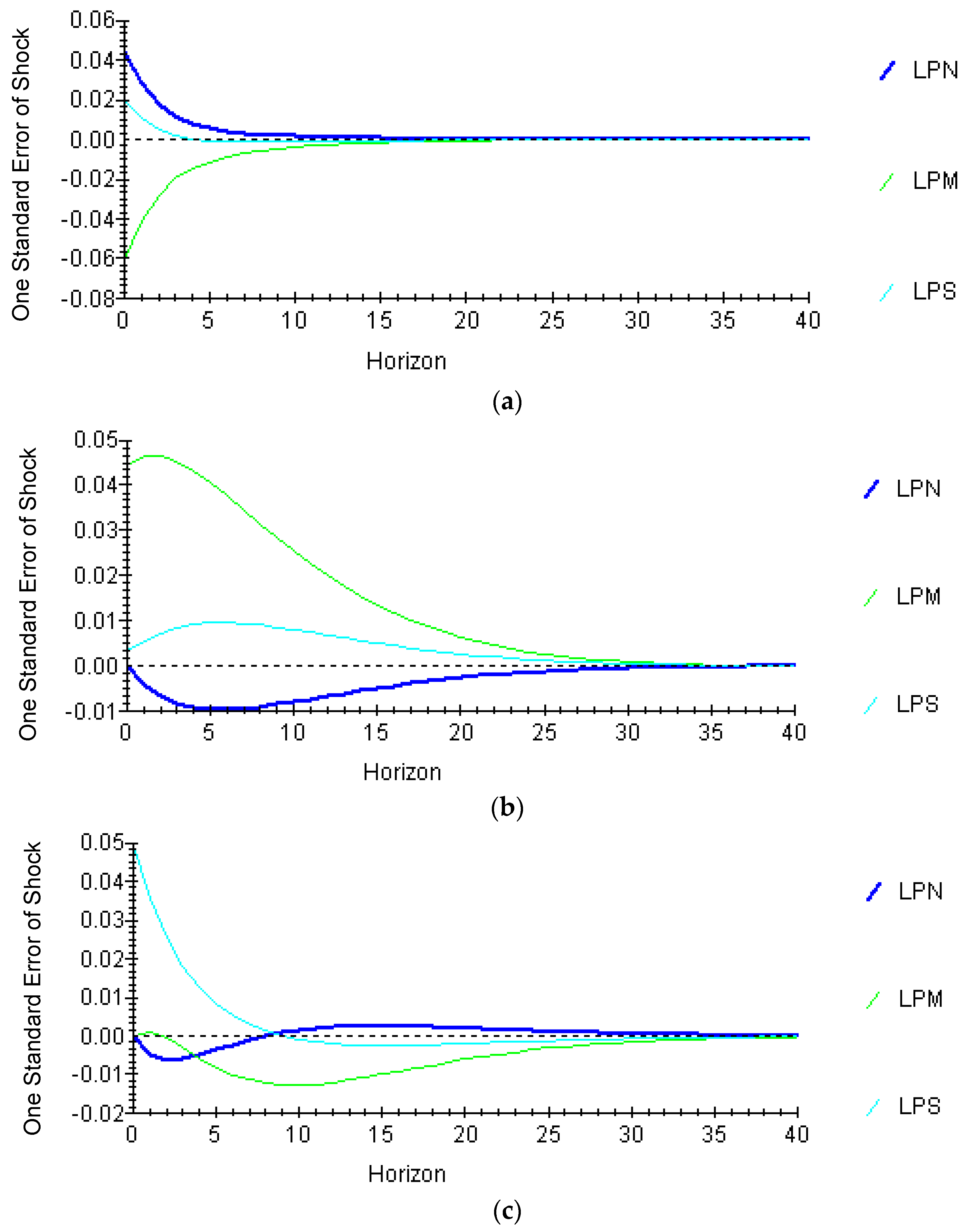
The impulse response functions are graphically illustrated in
Figure 2a–c. In
Figure 2a, a one standard-error (SE) shock to
LPN has an initial positive effect on
LPN and
LPS, while it has a negative effect on
LPM. The effect of
LPM and
LPN dissipates after 10 to 14 quarters, and the effect of
LPS by three quarters. In
Figure 2b, one SE shock on
LPM has an immediate positive effect on
LPM, which reaches a peak after two quarters then starts to decline steadily. The shock has also a positive impact on
LPS, which increases for about five quarters and then begins to fall. However, the shock has only small effects on
LPN. The shock on the prices tends to die out after 30 quarters. In
Figure 2c, one SE shock on
LPS also tends to die out after approximately 30 quarters, but the large initial effect is from
LPS compared to
Figure 2b.
Figure 2.
(a) Orthogonalized Impulse Responses to one Standard Error Shock in the LPN Equations; (b) Orthogonalized Impulse Responses to one Standard Error Shock in the LPM Equations; (c) Orthogonalized Impulse Responses to one Standard Error Shock in the LPS Equations.
Figure 2.
(a) Orthogonalized Impulse Responses to one Standard Error Shock in the LPN Equations; (b) Orthogonalized Impulse Responses to one Standard Error Shock in the LPM Equations; (c) Orthogonalized Impulse Responses to one Standard Error Shock in the LPS Equations.
4. Discussion
The direction of causality among the price variables has significant policy implications, especially for the design of price stabilization policies. For instance, if there is no causality, a price control can be implemented without the concern of any impact across regions. If a unidirectional causality running from at least one price to another exists, the interpretation is that the market with the unchanged price is the price-leader. As such, some form of price regulations on the price-leaders market will have an impact on the other markets. Obviously, price regulations will have an overall affect in case of bidirectional causality.
The general insight form the tests conducted reveals that the timber price variables are non-stationary and integrated by the first order. The structural break dummy is found to be statistically significant for the LPS equation. By and large, since the market is integrated, the effects of shocks tend to be mitigated because it induces trade between surplus and deficit areas. The scope for arbitrage across markets results in the spatial cancelling of harvest disturbances. Since the timber market is integrated and a harvest failure leads to a rise in one region, then producers exploit arbitrage opportunities by selling their goods in such regions. This will eventually lower the price in the latter region, while prices in other regions rise until equilibrium is reached. But even with an integrated market, a major disturbance like the storm Gudrun can severely disrupt the price equilibrium and lead to drastic shortages. Consequently, this displays the importance of controlling for shocks when performing the causality test.
As per the VECM-based causality, the central timber markets therefore occupy the leadership position in price formation and transmission. This result is not too surprising as the central market is the largest of the three in terms of harvesting volumes and will therefore exert significant influence in the evolution of other market prices [
47]. The variance decomposition and impulse response functions provide evidence that the markets are integrated and there is a certain degree of interdependency among them.
In general, the results which support the LOP hypothesis and market integration at the national level is in line with the Toppinen and Toivonen [
15] and Niquidet and Manley [
24] study of the wood market in Finland and New Zealand, respectively, but is in contrast to Daniels [
25], where no evidence of the LOP hypothesis was found for timber markets in the Western US. Since the Swedish timber markets are regionally integrated, they will be open to international integration and it could be expected that they develop a certain magnetism attracting trade from neighboring markets. Several studies have reported an integrated international Swedish timber market with other Scandinavian countries like Denmark [
12] and Finland [
12]).
5. Conclusions
The purpose of this paper was to assess the spatial price linkages in the spruce and pine markets in central, Northern, and Southern Sweden, using quarterly data over the period 1999Q1–2012Q4. Several unit root and cointegration tests have been computed. No evidence of seasonal effects is found and the variables are found to be integrated of first order and co-integrated, especially after controlling for a structural break. As such, the weak form of the LOP hypothesis is supported. Following, according to the VECM-based Granger-causality test, the central market emerges as the price-leader while variance decompositions and impulse response functions confirm the results about an integrated market and provide further evidence of price interdependency across markets.
This has interesting implications for the forecasted expansion of forest-based biofuel production. Firstly, since the LOP hypothesis cannot be rejected, the regional price effects from increased utilization will diffuse and will thus not be as large as expected if the regional markets were not integrated. Secondly, the geographical importance for establishing new production capacity, utilizing timber or its derivatives as feed-stock, is reduced, at least from a feed-stock procurement perspective.
Furthermore, it has implications for public and private decision-makers that need to understand market behavior and price determination mechanisms. For instance, since the timber markets in Sweden are integrated, they can be aggregated into a single national timber market. This will simplify the understanding on how the timber markets function in Sweden and facilitate general policies applied on a national level. That is, the use of aggregation is more appropriate for decision-makers since the timber markets are integrated.
These results can assist policy-makers in understanding the dynamics of the behavior of the timber market. Aggregation at the regional, national, or international level is often unavoidable. Since the markets are integrated, long-run aggregate market analysis is feasible [
19]. Moreover, the causality results have shed light on the process of price formation across regions and could be used in forecasting. Since the central market is acting as the price-leader, timber prices can be used to predict future prices in the Northern and Southern markets. Such knowledge can also be helpful in designing price stabilization programs whereby policies affecting the central market will affect the other two markets and not vice versa. In essence, market integration analysis can assist policy-makers in efficient long-term decision making.


