Accounting for a Diverse Forest Ownership Structure in Projections of Forest Sustainability Indicators

Eggers, Jeannette; Holmström, Hampus; Lämås, Tomas; Lind, Torgny; Öhman, Karin

doi:10.3390/f6114001

Open AccessArticle

Accounting for a Diverse Forest Ownership Structure in Projections of Forest Sustainability Indicators

Department of Forest Resource Management, Swedish University of Agricultural Sciences, Skogsmarksgränd, Umeå 90183, Sweden

^*

Author to whom correspondence should be addressed.

^†

These authors contributed equally to this work.

Forests 2015, 6(11), 4001-4033; https://doi.org/10.3390/f6114001

Submission received: 12 August 2015 / Revised: 29 October 2015 / Accepted: 30 October 2015 / Published: 6 November 2015

(This article belongs to the Special Issue Ecosystem Services from Forests)

Download

Browse Figures

Versions Notes

Abstract

:

In this study, we assessed the effect of a diverse ownership structure with different management strategies within and between owner categories in long-term projections of economic, ecological and social forest sustainability indicators, representing important ecosystem services, for two contrasting Swedish municipalities. This was done by comparing two scenarios: one where the diversity of management strategies was accounted for (Diverse) and one where it was not (Simple). The Diverse scenario resulted in a 14% lower total harvested volume for the 100 year period compared to the Simple scenario, which resulted in a higher growing stock and a more favorable development of the ecological indicators. The higher proportion of sparse forests and the lower proportion of clear-felled sites made the Diverse scenario more appropriate for delivering access to common outdoor recreation activities, while the Simple scenario projected more job opportunities. Differences between the scenarios were considerable already in the medium term (after 20 years of simulation). Our results highlight the importance of accounting for the variety of management strategies employed by forest owners in medium- to long-term projections of the development of forest sustainability indicators.

Keywords:

ecosystem services; forest management strategy; ownership structure; simulation

1. Introduction

Projections of forest resource development are important tools used for impact assessment; they provide both information about potential future resource supply and input into policy processes. Such projections are undertaken on the local, regional, national or larger scale [1,2,3,4]. In projections of future forest resource development, models are commonly used to simulate the possible development of forest resources and other forest ecosystem services over long time frames. Often, a number of different scenarios are compared, in order to gain an idea of possible future forest conditions given different assumptions about, for example, environmental and social drivers, such as growth impacts due to environmental changes, policy changes, or changes in management [5,6,7,8,9]. In recent years, ecosystem services, i.e., the benefits humans obtain from ecosystems, have received considerable attention in the scientific literature and in policy development [10], and efforts have been undertaken to develop indicators in order to map and evaluate different services [11]. Besides wood production, other ecosystem services, such as carbon sequestration and recreational value, have been allocated greater importance recently and are increasingly included in impact assessments [6]. However, in the majority of national or regional forest development studies, there are differences between the management guidelines that drive harvesting activities and actual management practices, and these may cause large discrepancies between expected and observed harvest, as well as other ecosystem services, even in short-term projections [12,13]. One reason for this is that, even though forest management objectives are known to vary substantially between owners [14,15], ownership structure is rarely taken into account in projections of forest resource development, and the impact of different ownership types and their inherent management schemes on forest ecosystems has been poorly studied so far [16,17]. Nonetheless, several studies indicate that ownership structure has a substantial impact on forest management. For example, Schaich and Plieninger [16] found that forests owned by small-scale private owners differed significantly from forests owned by the state and municipalities in terms of higher levels of structural diversity, deadwood and carbon storage capacity. The authors attribute this fact to less intensive and more diverse forest management in private forests, driven by the multitude of different objectives and management schemes of small-scale private forest owners. Arano and Munn [18] investigated landowners’ investment in forestry, as a proxy for management intensity, for different owner categories in Mississippi, USA. They found that non-industrial private forest (NIPF) owners spent significantly less money on silvicultural activities than industrial owners, implying that NIPF owners’ management intensity is lower. Johnson et al. [19] applied different management strategies in modeling forest structure in the Coast Range of Oregon, USA, for industrial, non-industrial, state and federal forests, and found that forest structure diverged increasingly over time between the different ownership types. Zheng et al. [20] found indications that the proportion of forest with high aboveground biomass was unevenly distributed across broad ownership categories, indicating that ownership behaviors influence carbon storage and other ecosystem services. Rinaldi et al. [17] propose a concept for integrating forest resource assessment and economic modeling of harvesting behavior, using a pan-European forest modeling framework taking into account different attitudes and objectives among forest owners. However, the approach is less suitable for the landscape or regional level, as it is rather coarse and, so far, only based on informed estimates. Further, the focus of the modeling approach is on timber yields, while its ability to quantify and project other forest ecosystem services is very limited.

In Sweden, about 23 million ha, i.e., half of the land area, is covered by productive forest (production capacity > 1 m³/ha/year), and forestry and the forest industry constitute an important part of the Swedish economy, making up 11% of the Swedish total export value and 2.2% of Swedish GDP [21]. Forestry was traditionally production-oriented in Sweden, but in 1994, a new Forestry Act came into force, giving environmental and production goals equal importance, and requiring all forest owners to take some nature consideration in their forest management, such as retaining trees/tree groups and buffer zones [22]. In 1999, the Swedish Parliament adopted several environmental objectives, including “Sustainable Forests” [23], aiming to preserve forest’s biodiversity, as well as cultural and social values. Social values, with a focus on recreation, have received increased attention during the last years [22,24].

In Sweden, about half of the productive forest area belongs to NIPF owners (i.e., individual owners, excluding privately-owned enterprises), with a higher proportion of NIPF owners in southern Sweden compared to northern Sweden. Private-owned enterprises hold 25% of the productive forest area, while the rest belongs to other owners such as the state and the Church [21]. In Sweden, forest owners are responsible for management decisions on their land, and forest legislation gives owners considerable freedom in their choice of forest management. Eggers et al. [25] showed that there is considerable variety in management strategies between NIPF owners, and that the single most important factor influencing choice of management strategy for NIPF owners in Sweden was property size. Despite this difference in management strategies between forest owners, regional and national assessments, such as forest impact analysis and future wood supply projections [2,26], regularly undertaken in Sweden, largely neglect the heterogeneous forest ownership structure and its impact on forest management. On the other hand, knowledge of potential development of forest ecosystem services is important for planning, including municipal planning, given municipalities’ responsibilities for maintaining a good environment for residents, and their commitment to Sweden’s environmental objectives. Municipalities play an important role in working towards these aims, by translating national and regional objectives to local objectives and action plans. Therefore, there is a need for forest scenario development, taking ownership considerations and their impact on management into account.

In this study, we describe a method for and assess the effect of taking into account the diversity of management strategies among different forest owner types. Two scenarios of forest resource development were compared: one where the diverse ownership pattern and resulting diversity in management practices was taken into account as much as feasible, and one simple scenario, only differentiating between protected forest, industrial and non-industrial forest, based on national assessments of forest resources in Sweden [2]. Differences in the modeled outcomes based on these two scenarios were then compared for a number of economic, ecological and social indicators representing important forest ecosystem services, for two municipalities in Sweden. As we encompass the difference in growing conditions and ownership structure between the northern and southern parts of Sweden in our choice of municipalities, we expect our outcomes to be relevant for other regions as well.

2. Material and Methods

2.1. Input Data

Growing conditions and forest ownership structure vary considerably on a north–south gradient in Sweden [21]. In the south, productivity is generally higher, due to a longer vegetation period, and the majority of the forest is owned by non-industrial private forest owners. In northern Sweden, a higher share of the productive forest area is owned by large private forest enterprises, and forest productivity is lower due to the harsh climate. Thus, rotations periods are generally longer in the north, and tree species composition differs—in the north, the main tree species are Scots pine, Norway spruce and birch, while in the southernmost part of Sweden, almost 30% of the growing stock consists of valuable broadleaved species, in particular beech and oak. In order to encompass these differences, we selected one municipality in northern Sweden (Vilhelmina) and one in southern Sweden (Hässleholm) as case study areas (Figure 1). In Hässleholm, belonging to the continental zone, the average length of the vegetation period is about 200 days, while it is only about 120 days in Vilhelmina, which is situated in the boreal/alpine zone (Table 1). Thus, forest productivity is much higher in Hässleholm compared to Vilhelmina, and there is a higher number of broadleaved species in Hässleholm.

Figure 1. Location of the Hässleholm and Vilhelmina municipalities within Sweden.

Table 1. Key facts about Hässleholm and Vilhelmina.

**Table 1.** Key facts about Hässleholm and Vilhelmina.
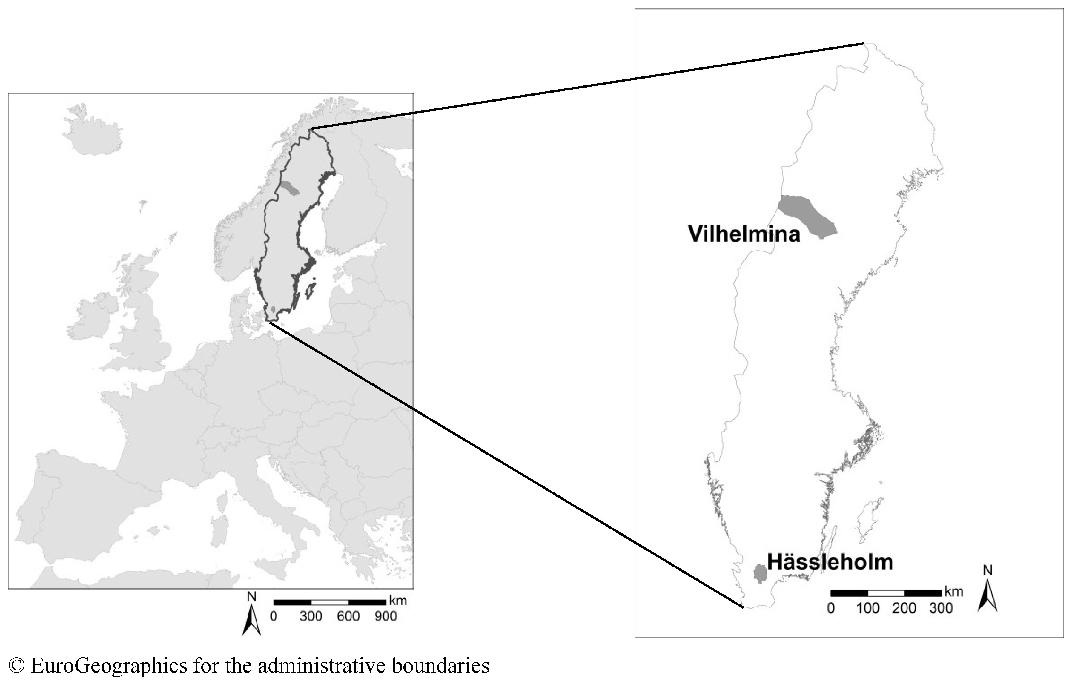
	Hässleholm	Vilhelmina	Source
Size (km²)	1306	8741	SCB [27]
Inhabitants (2014)	50,565	6848	SCB [28]
Biogeographical region	Continental	Boreal/Alpine	EEA [29]
Average length of vegetation period (days with average temperature > 5 °C)	200	120	SMHI [30]

Input data for the simulations were created using a country-wide forest map (raster format 25 × 25 m²) based on satellite data and field data of the national forest inventory (NFI) [31], divided into forest stands, and complementary data from NFI plots (such as site index, stem density and basal area) [32]. For Vilhelmina, the forest map of 2005 (SPOT 4 satellite) was used and complemented with information from NFI plots gathered during the years 2001–2005, while for Hässleholm the forest map of 2010 (SPOT 5 satellite) was available and in turn complemented with information from inventory plots gathered during 2005–2009. Thus, the input data for Vilhelmina represent the year 2003, and for Hässleholm, 2007. The input data was combined with cadastral maps (vector format) that provided information on ownership and property sizes [33], as well as a number of relevant environmental and administrative layers: key biotopes, nature reserves, Natura 2000 areas, bog forests, and zones where only continuous cover forestry is permitted, all in vector format, available at the data portals of the Swedish Forest Agency and the Swedish Environmental Protection Agency [34,35,36].

In Hässleholm, the productive forest area covers almost 73,000 ha. The majority of the forest (86%) is owned by NIPF owners (Table 2). The mean forest age is 45 years, with the majority of the forest being younger than 60 years, and very little forest (<2%) older than 120 years (Figure 2). The main tree species are Norway spruce (50%), European beech (14%), birch (11%) and Scots pine (9%) (Table 3).

Table 2. Ownership structure in Hässleholm and Vilhelmina.

**Table 2.** Ownership structure in Hässleholm and Vilhelmina.
Owner	Hässleholm		Vilhelmina
Owner	Productive Forest Area (ha)	Share (%)	Productive Forest Area (ha)	Share (%)
NIPF owners	62,721	86	121,534	39
Municipality ¹	2,937	4	5,969	2
Church	2,636	4	1,694	1
Forest enterprise	2,270	3	70,705	22
Foundations	2,006	3	0	0
National Property Board	0	0	80,450	26
Forest commons	0	0	34,487	11
Total	72,570	100	314,839	100

¹ Including HIBAB, a municipality-owned enterprise.

In Vilhelmina, there are about 315,000 ha of productive forest area. Almost 40% of the productive forest is owned by NIPF owners, while the remaining area is owned by various forest enterprises (including Sveaskog, a state-owned enterprise), forest commons, the state and the church (Table 2). For municipality forest, the original input data were updated with more detailed forest stand descriptions from Nilsson (2014) [37]. For the National Property Board of Sweden, four different forest management objective classes, available from their website [38], were added to the stand description. The mean age of the forest is 73 years, with a relatively even distribution over age classes, and 24% of the forest is older than 120 years (Figure 2). The main tree species in Vilhelmina are Norway spruce (57%), Scots pine (27%) and birch (13%) (Table 3).

Figure 2. Initial age class distribution in Hässleholm (left) and Vilhelmina (right). NB: different scales on y-axes.

Table 3. Initial tree species distribution in Hässleholm and Vilhelmina.

**Table 3.** Initial tree species distribution in Hässleholm and Vilhelmina.
Tree species	Volume (1000 m³)		Share (%)
Tree species	Hässleholm	Vilhelmina	Hässleholm	Vilhelmina
Scots pine (Pinus sylvestris)	1,035	7,548	9	27
Norway spruce (Picea abies)	5,528	15,793	50	57
Birch (Betula pubescens and B. pendula)	1,187	3,713	11	13
Aspen (Populus tremula)	100	236	1	1
Oak (Quercus robur)	806	0	7	0
European beech (Fagus sylvatica)	1,571	0	14	0
Other valuable broadleaves	249	0	2	0
Lodgepole pine (Pinus contorta)	0	127	0	0
Other broadleaves	587	215	5	1
Total	11,063	27,633	100	100

2.2. The Heureka Forest Model

In this study, the Heureka forestry decision support system was used to project the development and output of goods and services from the forest for 100 years in steps of five years, from the start year 2003 or 2007 in Vilhelmina and Hässleholm, respectively. The Heureka system, recently developed at the Swedish University of Agricultural Sciences [39], is widely used in Sweden for the analysis and planning of forest management, both by scientists and forestry professionals. In this study, the RegWise module of the Heureka system (version 2.2.0.9) was used. RegWise is a simulation model especially suited for impact analysis on a regional or national level. Data on present forest condition (including age-class and tree-species distribution) as well as ecosystem processes are used to predict the future forest condition, given a set of user-defined management actions and taking legal requirements into account. RegWise was here applied in a spatially explicit mode projecting the development of individual stands. The central drivers of the Heureka system are empirical growth models, mainly developed using data from the NFI and applicable on all Swedish tree species. The models are applicable also on mixed species stands and have been shown to provide reliable growth predictions for up to 100 years [40]. The growth models are complemented by models regulating, inter alia, natural mortality [32] and in-growth [41]. Logistic regression functions are used to calculate the probability of silvicultural activities being undertaken, based on the analysis of permanent NFI plots [42]. At the same time, the user has great freedom to direct and constrain management activities, for example by specifying the minimum age for final felling, the type of regeneration, the timing and intensity of thinnings, the maximum share of net annual growth to be harvested, as well as the amount of forest set-aside for nature conservation.

2.3. Model Set-Up

Two different scenarios were constructed: Diverse and Simple. In both scenarios, sets of different management actions were defined. In the Simple scenario, we assigned different management strategies to protected areas, NIPF owners, and other owners. In the Diverse scenario, we differentiated in more detail, and implemented five different management strategies for NIPF owners (based on [25]), and applied more differentiation to other owners (e.g., municipalities, forest commons, forest enterprises). Eggers et al. [25] found that the single most important factor influencing NIPF owners in their choice of management strategy was property size, with owners of larger properties more frequently adopting production-oriented management strategies. We therefore differentiated between three different property size classes for NIPF owners, and for each size class, forest stands were randomly assigned a management strategy, based on proportions from Eggers et al. [25]. The strategies were as follows:

•: Passive (“I thin and clear-cut only on a small scale. I let the forest grow old, but I do not expect the harvest to increase in the future.”),
•: Conservation (“I harvest only on a small scale, so that the amount of old forest remains constant or increases. My management practices are oriented towards nature protection, for example to increase the proportion of broadleaved forest.”),
•: Intensive (“I harvest a lot of wood by thinning, and I clear-cut as soon as the forest age permits.”),
•: Productivity (“I manage the forest for increased productivity and future harvest opportunities. Examples of my management practices are planting with soil scarification, pre-commercial thinning, ditching and fertilization.”), and
•: Save (“I harvest carefully and my management practices aim to increase harvest opportunities in the medium term.”).

For both scenarios, forest in key biotopes, nature reserves and Natura 2000 areas was left unmanaged irrespective of owner type. The default pricelists within the Heureka system were updated with prices from the Södra forest owners’ association [43] for Hässleholm, and with prices from the Norra forest owners’ association for Vilhelmina [44], and cost functions based on Brunberg (1995, 1997, 2004) [45,46,47] were used. For forests dominated by selected valuable broadleaved species (oak, beech, ash, elm, lime, maple), harvesting costs for final fellings were doubled to account for the higher cost of motor-manual fellings, which is the common final felling method for these tree species. The discount rate, used to calculate the net present value, was set at 1.5% in both scenarios.

The distribution of forest area over the different management strategies in the Diverse scenario is given in Table 4 and Table 5. In the Simple scenario, protected areas were assigned to the no management strategy, non-industrial private forest owners to the Simple-NIPF strategy, and other owners to the Simple-other strategy in both municipalities. In Vilhelmina, forest above the final felling threshold was managed as in the Diverse scenario, with continuous cover forestry. Management focus is on recreation to a large extent in forest owned by the municipality and foundations in Hässleholm, which is why a shelterwood management strategy was assigned to a large proportion of this forest in the Diverse scenario. Also in Vilhelmina, some of the municipal forest is managed without clear-felling [37], which is why the forest dominated by spruce in this zone was assigned a continuous cover forestry regime, and the forest dominated by pine and birch was assigned to the shelterwood management strategy in the Diverse scenario. The management strategies are described in Table 6. For all management strategies (unless otherwise stated), nature conservation was set as demanded by certification: 5% of the productive area was set-aside with no management (randomly allocated), and 10 live trees and 3 high stumps per ha were left on final felling sites, with a priority on retaining large-diameter trees [48].

Table 4. Distribution of management strategies for the different owner and forest types in the Diverse scenario (Hässleholm).

**Table 4.** Distribution of management strategies for the different owner and forest types in the Diverse scenario (Hässleholm).
Owner	Forest Type/Size Class	Management Strategy
Owner	Forest Type/Size Class	No mgmt.	Passive	Conservation	Intensive	Productivity	Save	Shelterwood
All	Protected	100%	-	-	-	-	-	-
All	Bog forests	-	-	100%	-	-	-	-
NIPF	0–20 ha	-	37%	16%	4%	7%	36%	-
	21–50 ha	-	18%	10%	16%	25%	31%	-
	>50 ha	-	5%	4%	18%	49%	24%	-
Other	Forest enterprise	-	-	-	-	100%	-	-
	Municipality	-	-	50%	-	-	-	50%
	Foundations	-	-	50%	-	-	-	50%

Table 5. Distribution of management strategies for the different owner and forest types in the Diverse scenario (Vilhelmina).

**Table 5.** Distribution of management strategies for the different owner and forest types in the Diverse scenario (Vilhelmina).
Owner	Forest Type/Size Class	Management strategy
Owner	Forest Type/Size Class	No Mgmt.	Passive	Conservation	Intensive	Productivity	Save	Shelterwood	CCF
All	Protected	100%	-	-	-	-	-	-	-
All	Above final felling threshold	25%	-	-	-	-	-	-	75%
NIPF	0–20 ha	-	34%	10%	4%	12%	40%	-	-
	21–50 ha	-	33%	4%	10%	26%	27%	-	-
	>50 ha	-	15%	8%	7%	43%	27%	-	-
Other	Forest enterprise	-	-	-	-	100%	-	-	-
	Municipality ¹	-	-	-	-	85%	-	7%	8%
	Forest commons ²	-	100%	-	-	-	-	-	-
	National Property Board ³	-	-	12%	-	74%	-	-	14%

¹ Zones and management developed in another study were used [26]; ² For the forest commons in Vilhelmina, currently about one quarter of the net annual increment is harvested [37], which is why the passive management strategy was chosen; ³ Forest management was implemented according to the four different forest management objective classes available for this forest owner.

Table 6. Description of management strategies.

**Table 6.** Description of management strategies.
Management Strategy	Description
No management	The forest is left unmanaged for natural development.
Passive	The rotation period is extended by 20%, and only 30% of the net annual increment is harvested. No pre-commercial thinnings are implemented, and commercial thinnings are less common, with a maximum of only 10% of the total harvested volume coming from thinnings. Forest dominated by selected valuable broadleaved species was left unmanaged.
Conservation	The rotation period is extended by 50%, and at least 20% of the area is left for natural development (set-aside). During pre-commercial and commercial thinnings, a 30% minimum share of broadleaves is maintained.
Intensive	For this management strategy, the only change to the default configuration was that the minimum final felling age was set according to legislation, i.e., there was no rotation period extension.
Productivity	The forest is mostly regenerated through plantation with trees from breeding programs, largely spruce. Scots pine was used only on the driest sites. In Vilhelmina, fertilizer is applied and Lodgepole pine is planted to some extent where allowed.
Save	The rotation period is extended by 50%. Thinnings are allowed up to a maximum tree height of 30 m (instead of 25 m) and even in older forests (up to a relative age of 1.5).
Shelterwood	The forest is regenerated with shelterwood to a great extent, and the rotation period is extended by 50%.
CCF	Continuous cover forestry: No final fellings take place; instead the forest is managed through a continually repeated series of selective harvests.
Simple—NIPF	Parameters for the regeneration method, species and soil scarification method, tree breeding and set-aside for nature conservation were taken from the reference scenario of the latest available national forest impact analysis [2]. Minimum final felling age was set according to legislation, i.e., there was no rotation period extension. In addition to protected unmanaged forest (key biotopes, nature reserves and Natura 2000), 8.1% of the productive forest area was set-aside for nature conservation in Hässleholm, and 4.2% in Vilhelmina.
Simple—Other	Parameters for the regeneration method, species and soil scarification method, tree breeding and set-aside for nature conservation were taken from the reference scenario of the latest available national forest impact analysis [2]. In addition to protected unmanaged forest (key biotopes, nature reserves and Natura 2000), 18.1% of the productive forest area was set-aside for nature conservation in Hässleholm, and 3.7% in Vilhelmina.

2.4. Sensitivity Analysis

The sensitivity of the Diverse scenario to subjective interpretation of the NIPF owner’s management strategies from [19] was tested by changing the most influential parameters: rotation length, harvest level and proportion of set-aside, creating two alternatives for the Diverse scenario, one with more intensive management (Diverse_m) and one with less intensive management (Diverse_l) (Table 7). The applied parameter changes were meant to span a considerable, but still plausible range of parameter settings [49].

Table 7. Model parameters for the Diverse scenario and its alternatives for the sensitivity analysis: more intensive management (Diverse_m) and less intensive management (Diverse_l).

**Table 7.** Model parameters for the Diverse scenario and its alternatives for the sensitivity analysis: more intensive management (Diverse_m) and less intensive management (Diverse_l).
	Diverse	Diverse_m	Diverse_l
Passive
Harvest level	30%	50%	10%
Rotation extension	20%	-	40%
Nature conservation
Rotation extension	50%	30%	70%
Set-aside	20%	10%	30%
Intensive & Productivity
Rotation extension	-	-	20%
Save
Rotation extension	50%	30%	70%
Shelterwood
Rotation extension	50%	30%	70%

2.5. Scenario Comparison

The scenarios were compared for a number of economic, ecological and social indicators (Table 8). We considered differences in indicator outcome to be relevant when the difference between the Diverse (Diverse_m, Diverse_l) and the Simple scenario exceeded 10%, marked when the difference exceeded 25%, and large when the difference exceeded 50%. Most of the indicators can be coupled to one or several ecosystem services [11] that are highly relevant in the region [50]. The harvest level indicates how much raw wood is harvested and available to the forest industry. Harvested wood is an important ecosystem service in Sweden, as forest products correspond to 11% of the total Swedish export, while forestry and the forest industry comprise 2.2% of the Swedish gross domestic product [21]. Forest growth is a measure of the forest’s productivity and thus the sequestering of carbon, while growing stock is a basic indicator for the assessment of the sustainability of forest management [51], which can be converted to carbon stored in living trees by the use of biomass expansion factors [52]. Climate regulation through carbon sequestration and storage is an important forest ecosystem service, which is affected by forest management practices to a large extent [53]. Net present value (NPV) allows for scenario comparison in economic terms, with respect to management activities. In northern Sweden, forests are used both for wood production and reindeer herding. Modern forest management practices are often detrimental to reindeer husbandry and especially during the winter months, reindeer food availability (mostly lichen) can be a problem. The indicator “potential reindeer winter pasture” [54], only used in Vilhelmina, includes forest stands where ground lichen suitable for reindeer winter fodder may be found. Old forest, large trees and deadwood are important for maintaining biodiversity in a landscape [55,56], providing substrate and habitat for a large number of species, including many red-listed species [57]. Broadleaved trees are also highly associated with red-listed species in Sweden [57]. Boreal forests in a near-natural state have more large-diameter trees compared to managed forests [58], and the occurrence of large trees has been used as a biodiversity indicator in a number of studies [56,59]. Many species are deadwood-dependent, and deadwood is therefore widely used as a biodiversity indicator [60,61]. The indicators “mature forest with a high share of broadleaves”, “old forest” and “fresh deadwood” are also included as indicators for monitoring progress towards the Swedish environmental objective “Sustainable Forests” [23]. Some of the ecological indicators also serve as social indicators, such as old forests, which are valuable both for biodiversity and recreation. The social indicators include sparse forests, which are valuable for recreation, due to good visibility within them [62], and clear-cut areas. Large, fresh clear-cuts are considered a negative feature by the majority of forest visitors, while seed or retention trees can improve people’s perception of a felling site [63]. Recreational activities in forests, including walking, jogging, berry and mushroom picking, as well as hunting, are very common both in Sweden and other boreal countries [63,64]. Areas valuable for recreation are also important for nature-based tourism, a sector which is expected to grow in Sweden [65]. “Person-years” indicates employment potential in forest management, excluding the forest industry, which is especially important in rural areas.

Table 8. Description of the indicators that were used to compare the Simple and Diverse scenarios.

**Table 8.** Description of the indicators that were used to compare the Simple and Diverse scenarios.
Indicator	Description	Related Ecosystem Services
Economic
Total harvest (1000 m³ over bark/year)	Annual volume harvested in final fellings, thinnings, selective fellings, shelterwood fellings and seed tree removal	Raw materials
Net present value (SEK)	Sum of the present values of benefits and costs over 100 years with an interest rate of 1.5%
Growing stock (m³/ha)	Mean standing volume of living trees, above stump, over-bark	Climate regulation
Growth (m³/ha/year)	Net annual volume increment (growth—natural mortality)	Climate regulation
Potential reindeer winter pasture (%)	Share of productive forest area that is potentially available for reindeer winter grazing, according to an indicator developed in [39]	Food provision
Ecological
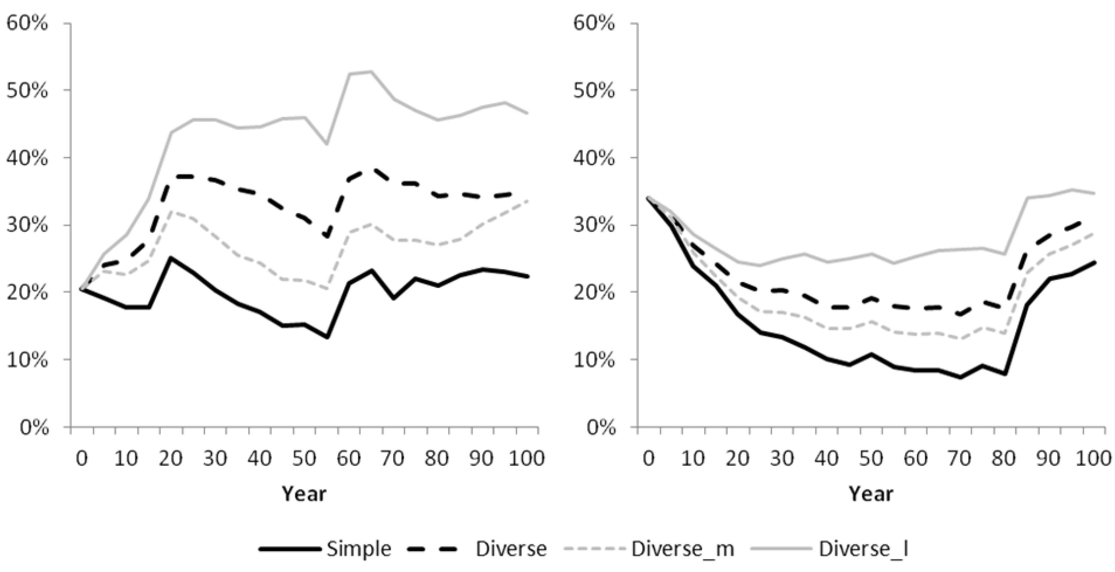
Mature forest with high share of broadleaves (%)	Proportion of productive forest area with a mean stand age of more than 60 years in Hässleholm, and more than 80 years in Vilhelmina, where broadleaves make up at least 25% of the basal area. Such forest is also valuable for recreation.	Lifecycle maintenance
Old forest (%)	Share of productive forest area with a mean stand age of more than 120 years in Hässleholm, and more than 140 years in Vilhelmina. Old forest is also valuable for recreation.	Lifecycle maintenance
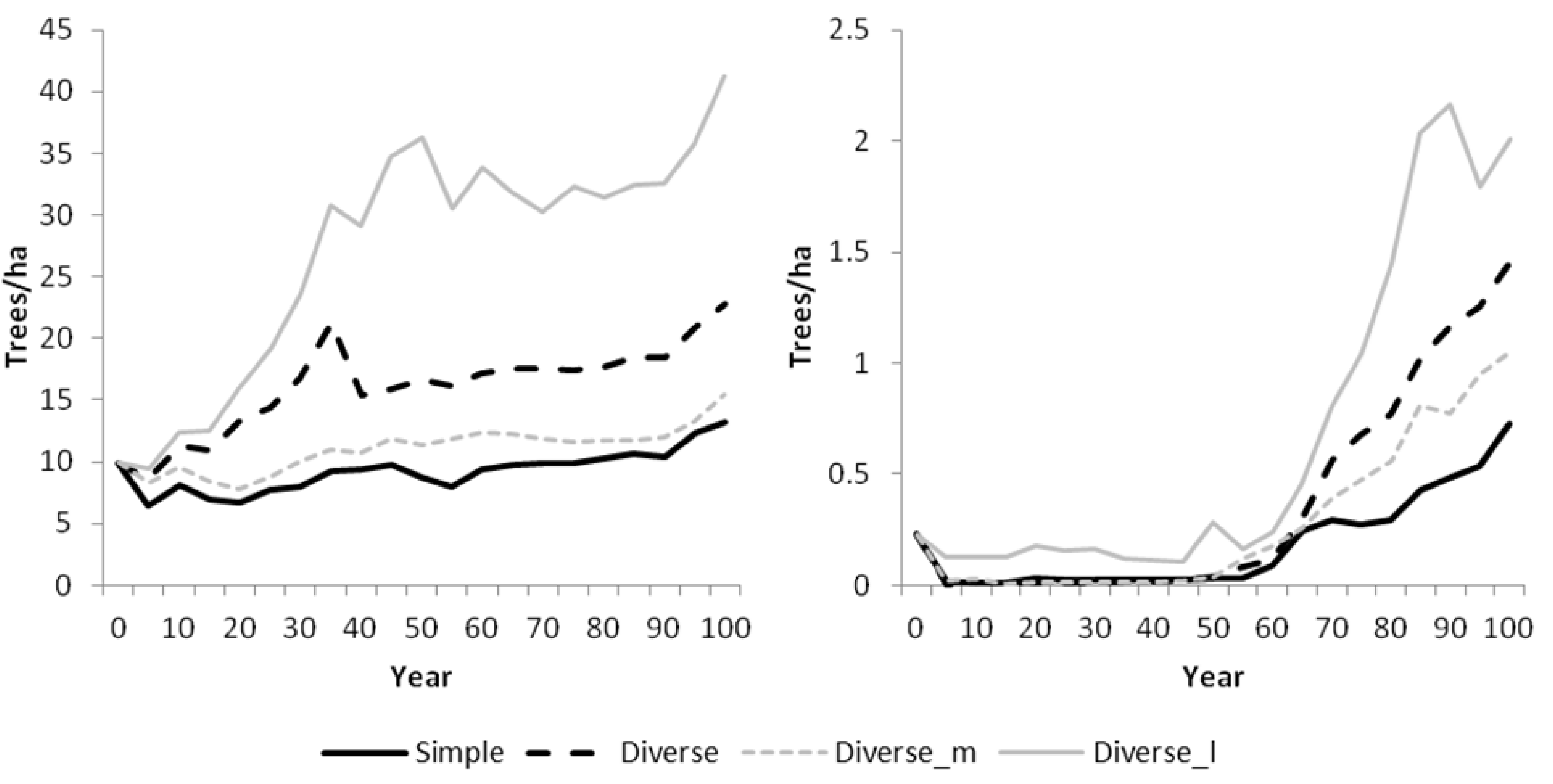
Large diameter trees (trees/ha)	Density of trees with a diameter >40 cm at breast height.	Lifecycle maintenance
Fresh deadwood (m³/ha)	Deadwood with a diameter >10 cm, with a very low level of decomposition: decay classes 0 and 1 according to the Swedish National Inventory [47].	Lifecycle maintenance
Social
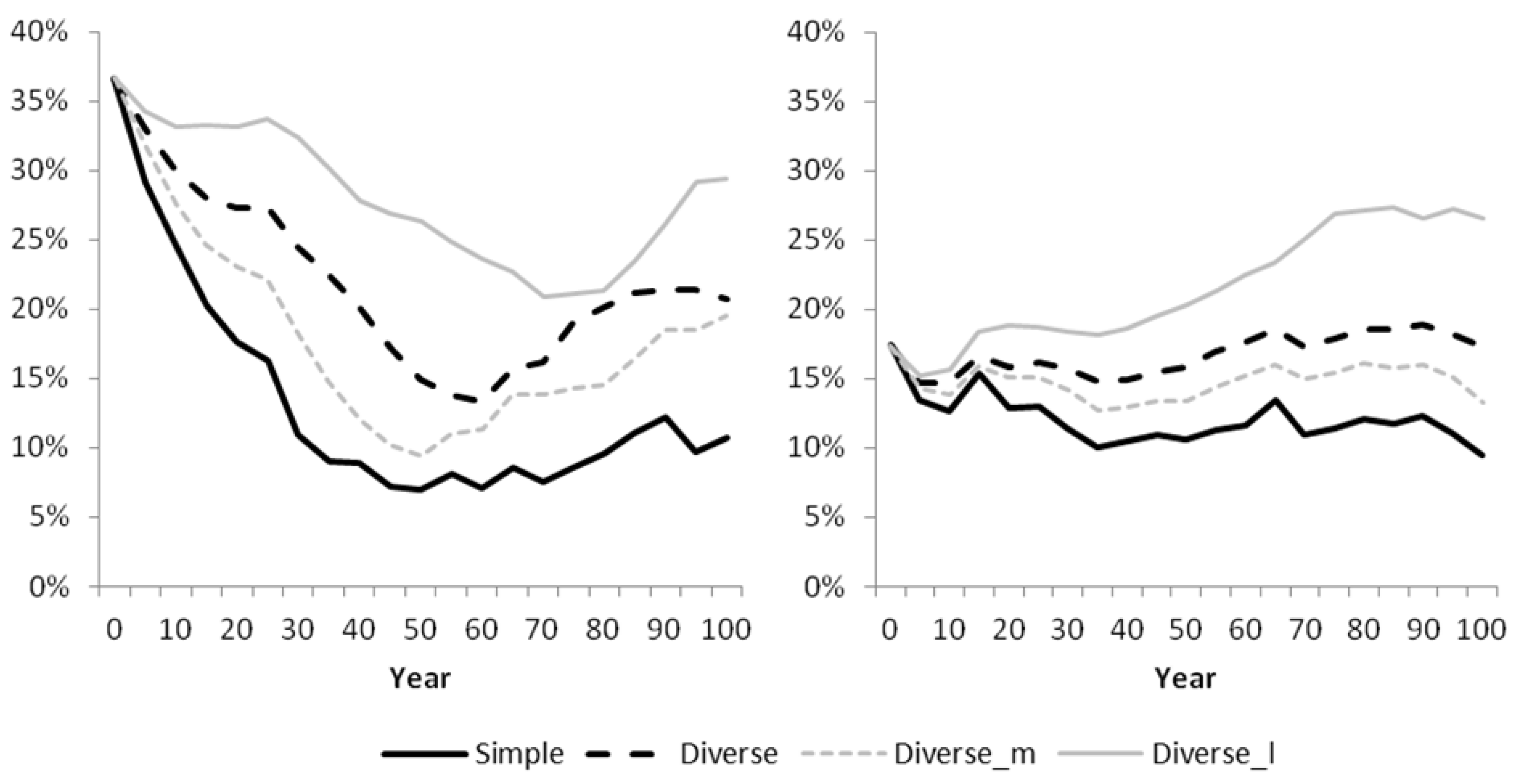
Sparse forest (%)	Proportion of productive forest area with less than 1000 stems per ha and a mean stand height > 10 m.	Aesthetic enjoyment, Recreation and tourism
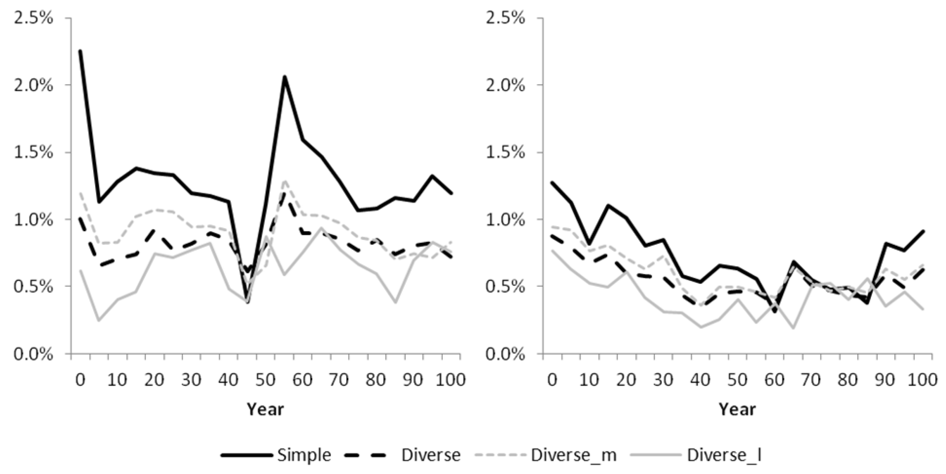
Clear-cut area (%)	Proportion of productive forest area that is subject to clearcutting annually (excluding regeneration areas with seed or shelter tree retention).	Aesthetic enjoyment, Recreation and tourism
Person-years (years)	Number of person-years (full-time employment, 1800 h work/year) needed for forest management activities (including soil scarification, planting, pre-commercial thinning, thinning, selective cutting, final felling, shelterwood/seed tree removal, timber transport to road-side)

3. Results

The results shown below are for productive forest area only, excluding protected, unmanaged areas such as nature reserves.

3.1. Economic Indicators

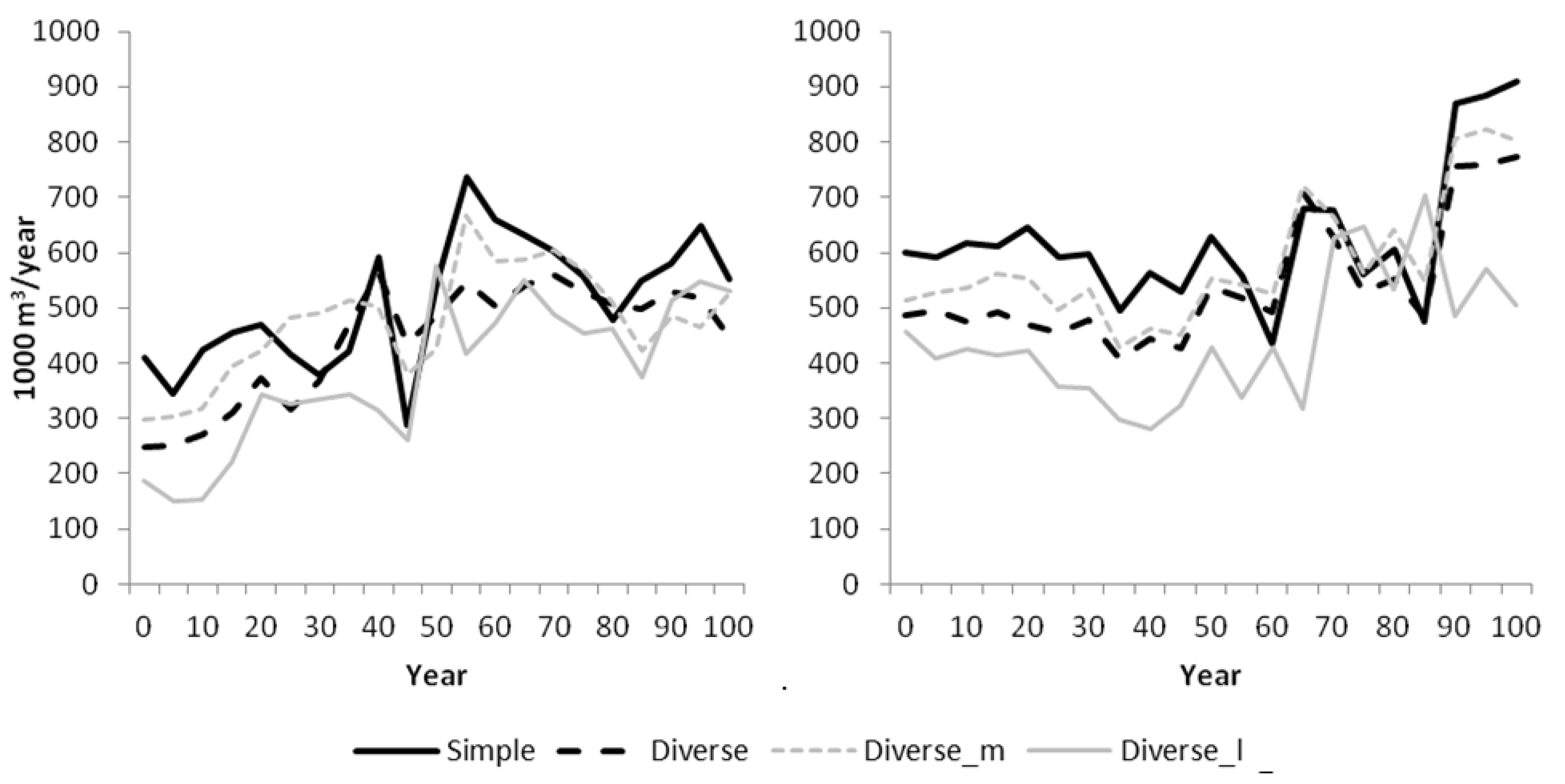
3.1.1. Total harvest Volume and NPV

In both scenarios, there was, in general, a rising trend in harvest levels over time. Total harvest was higher for the Simple scenario for most of the 100-year period compared to the Diverse scenario, both in Hässleholm and in Vilhelmina (Figure 3). In total, harvest levels were around 14% lower on average for the 100 year period, for the Diverse scenario, in both municipalities (Table 9). The lower harvest level in the Diverse scenario resulted in a lower NPV in that scenario (Table 9).

Figure 3. Development of total harvest volume (1000 m³/year) in Hässleholm (left) and Vilhelmina (right) for the Simple and Diverse scenarios, as well as the more intensive (Diverse_m) and less intensive (Diverse_l) variations of the Diverse scenario.

Table 9. Net present value (NPV) and mean annual harvest in Hässleholm and Vilhelmina.

**Table 9.** Net present value (NPV) and mean annual harvest in Hässleholm and Vilhelmina.
Scenario	NPV (SEK per ha)		Mean Annual Harvest (1000 m³)
Scenario	Hässleholm	Vilhelmina	Hässleholm	Vilhelmina
Simple	73954	14956	511	625
Diverse	64359	12254	441	541
Diverse_m	69161	13402	474	581
Diverse_l	55344	9710	382	443

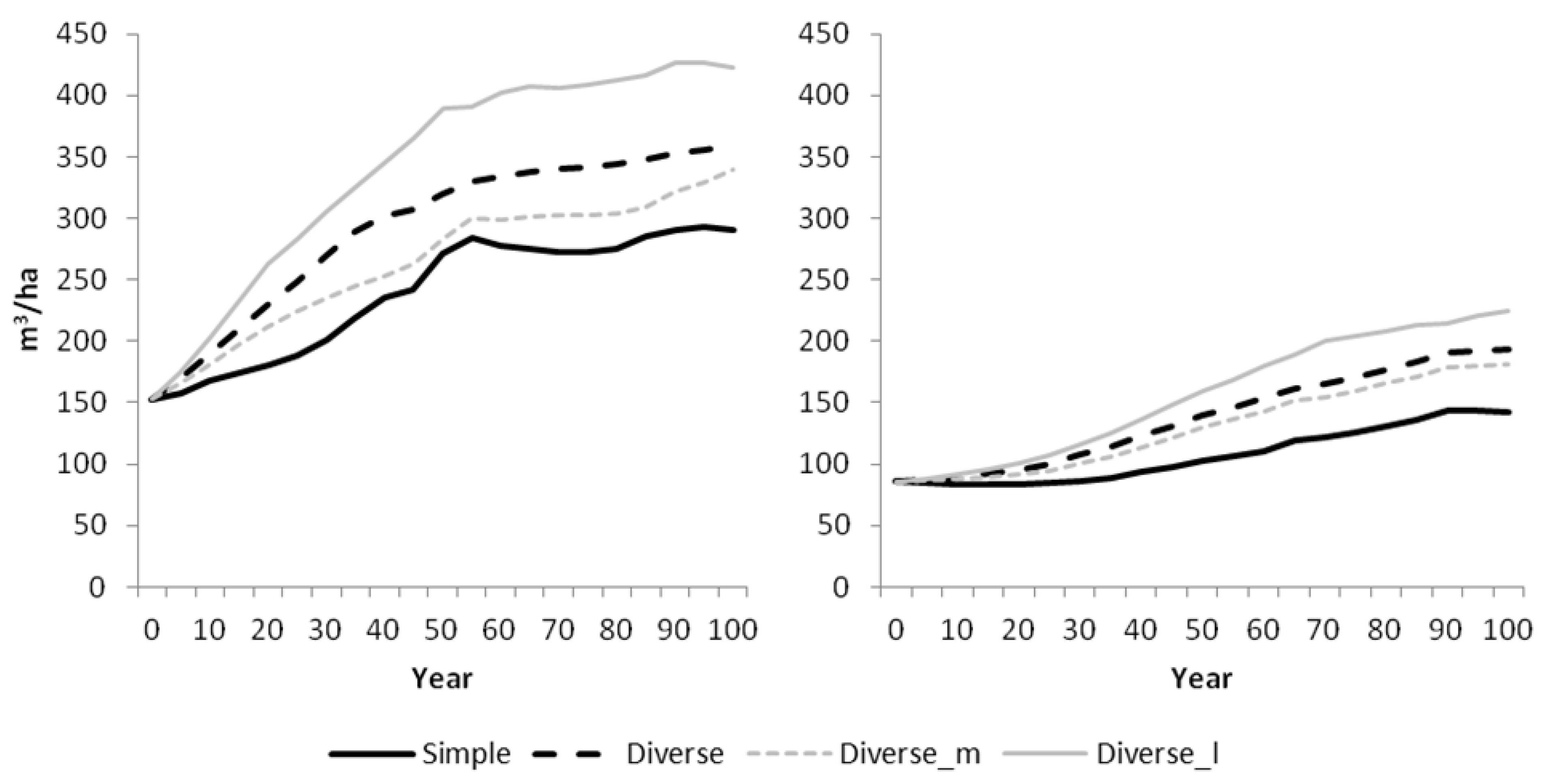
3.1.2. Growing Stock

For both scenarios, the growing stock increased markedly in both Hässleholm and Vilhelmina (Figure 4). However, the increase was more pronounced for the Diverse scenario and its alternatives, compared to the Simple scenario, due to the lower harvest level in the Diverse scenario. In Hässleholm, average growing stock increased to more than 350 m³/ha for the Diverse scenario, and to almost 300 m³/ha for the Simple scenario, after 100 years. In Vilhelmina, growing stock increased to almost 150 m³/ha in the Simple scenario, and almost to 200 m³/ha in the Diverse scenario, from its current level of 86 m³/ha.

Figure 4. Development of growing stock (m³/ha) in Hässleholm (left) and Vilhelmina (right) for the Simple and Diverse scenarios, as well as the more intensive (Diverse_m) and less intensive (Diverse_l) variations of the Diverse scenario.

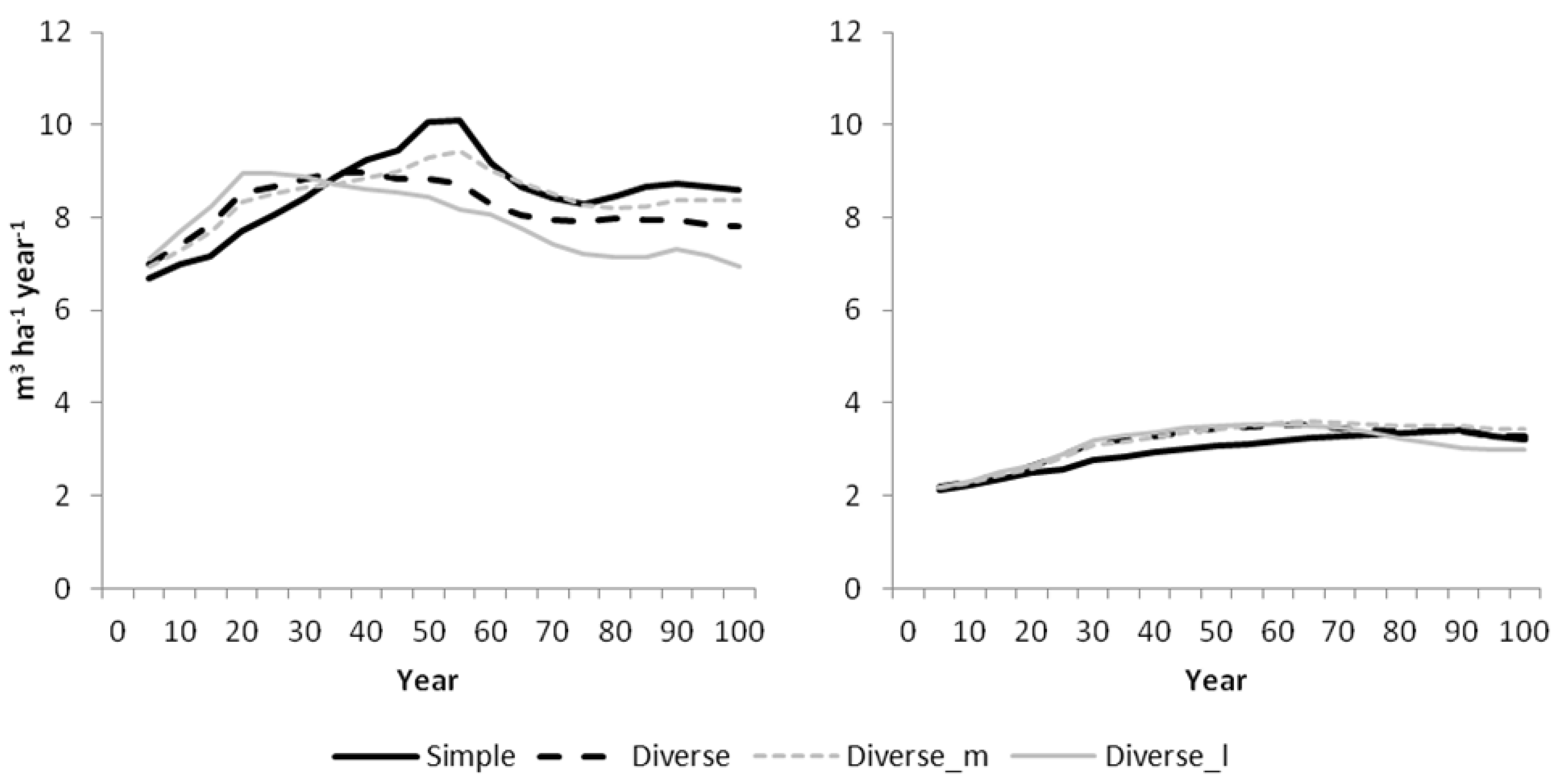
3.1.3. Growth

In both municipalities, differences in growth between the scenarios were quite small (Figure 5). In Hässleholm, growth increased in the first few decades, but for a longer time and to a higher level for the Simple scenario compared to the Diverse scenario. In contrast, annual growth was slightly higher for the Diverse scenario in Vilhelmina for most of the simulation period, even though the difference between the two scenarios decreased towards the end of the 100-year time span. For the low-intensity management alternative of the Diverse scenario, the increment dropped below the level of the Simple scenario towards the end of the simulation period, probably due to the large proportion of old forests in that scenario.

Figure 5. Development of the net annual volume increment (m³/ha/year) in Hässleholm (left) and Vilhelmina (right) for the Simple and Diverse scenarios, as well as the more intensive (Diverse_m) and less intensive (Diverse_l) variations of the Diverse scenario.

3.1.4. Potential Reindeer Winter Pasture

In both scenarios, potential reindeer winter pasture (defined as in [39]) decreased substantially, from around 14% at the beginning of the simulation to around 3%–4% at the end (Figure 6), with only small differences between the two scenarios, and between the two sensitivity runs. The most dramatic decrease occurred during the first 25 years.

Figure 6. Share of area that is potentially suitable for reindeer winter pasture in Vilhelmina, for the Simple and Diverse scenarios, as well as the more intensive (Diverse_m) and less intensive (Diverse_l) variations of the Diverse scenario.

3.2. Ecological Indicators

3.2.1. Mature Forest with a High Share of Broadleaves

The proportion of mature forest with a large proportion of broadleaves was higher in the Diverse scenario and its alternatives compared to the Simple scenario, throughout the simulation period for both Hässleholm and Vilhelmina (Figure 7). While the proportion of this type of forest remained largely constant (Simple scenario) or increased (Diverse scenario) in Hässleholm over time, it decreased in Vilhelmina for both scenarios for about 50 years, before increasing again towards the end of the simulation period.

Figure 7. Proportion of mature forest with large proportion of broadleaves, in Hässleholm (left) and Vilhelmina (right), for the Simple and Diverse scenarios, as well as the more intensive (Diverse_m) and less intensive (Diverse_l) variations of the Diverse scenario.

3.2.2. Old Forest

The proportion of old forest was projected to increase for both scenarios in Hässleholm, from below 2% at the beginning of the simulation, to 7% and 13% after 100 years, for the Simple scenario and the Diverse scenario, respectively (Figure 8). In Vilhelmina, the proportion of old forest decreased somewhat at the beginning of simulation for the Diverse scenario, remaining almost constant after 2025. In the Simple scenario, however, the share of old forest decreased to 3% in the middle of the 21st century, remaining almost constant thereafter. The difference in proportion of old forest between the two scenarios was considerable, with around three times more old forest under the Diverse scenario during the latter half of the simulation period in Vilhelmina.

Figure 8. Proportion of old forest in Hässleholm (left) and Vilhelmina (right), for the Simple and Diverse scenarios, as well as the more intensive (Diverse_m) and less intensive (Diverse_l) variations of the Diverse scenario.

3.2.3. Large Diameter Trees

In Hässleholm, the average number of large trees (diameter at breast height > 40 cm) changed only slightly in the simple scenario, while it increased markedly in the Diverse scenario (Figure 9). In Vilhelmina, there were hardly any large trees at the beginning, and their number started increasing only in the second half of the simulation period, more markedly for the Diverse scenario.

Figure 9. Average number of large trees per ha in Hässleholm (left) and Vilhelmina (right), for the Simple and Diverse scenarios, as well as the more intensive (Diverse_m) and less intensive (Diverse_l) variations of the Diverse scenario. NB: different scales on y-axes.

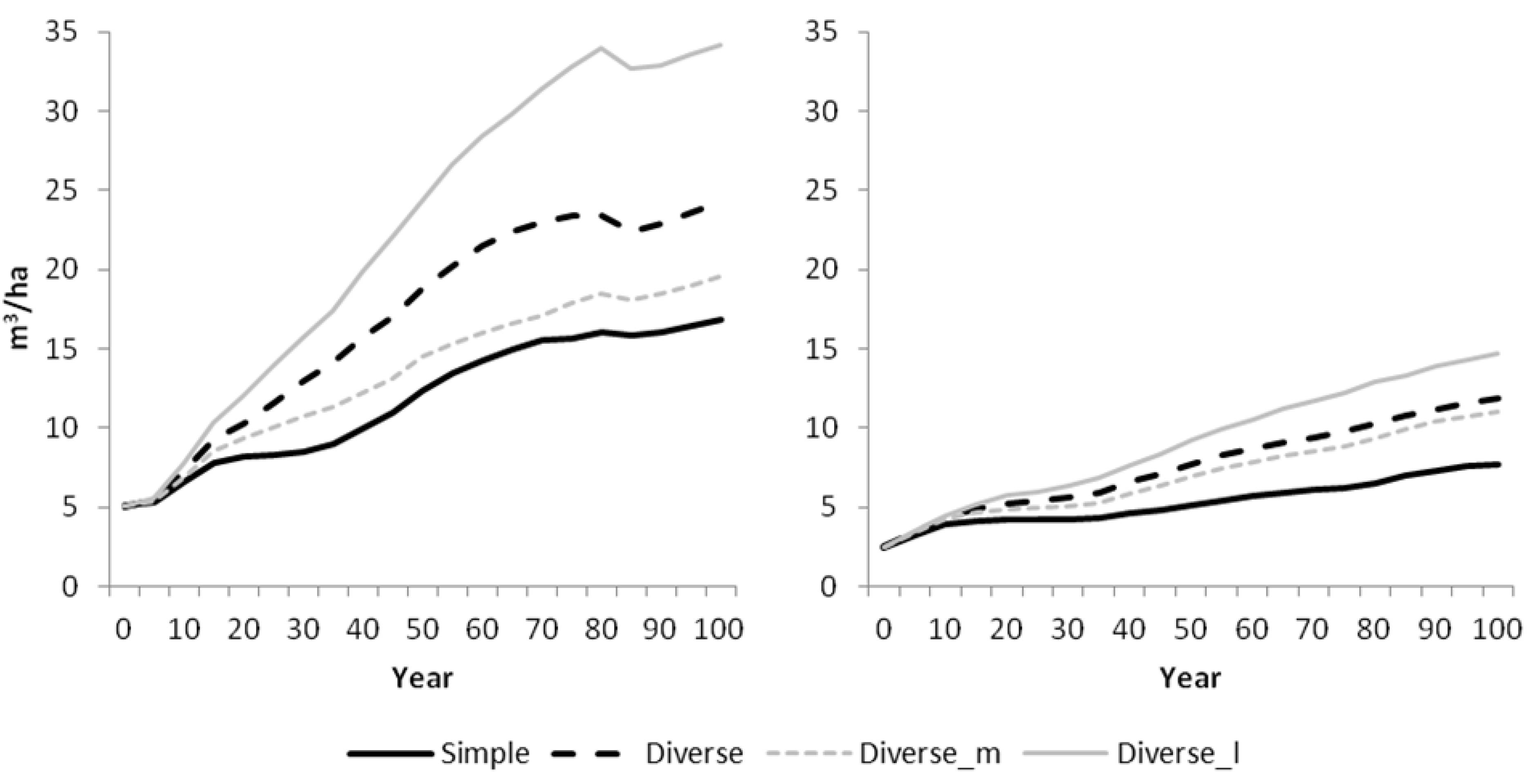
3.2.4. Fresh Deadwood

Fresh standing and lying deadwood was projected to increase in both Hässleholm and Vilhelmina, and for both scenarios, though more markedly for the Diverse scenario (Figure 10).

Figure 10. Fresh standing and lying deadwood (m³/ha) in Hässleholm (left) and Vilhelmina (right), for the Simple and Diverse scenarios, as well as the more intensive (Diverse_m) and less intensive (Diverse_l) variations of the Diverse scenario.

3.3. Social Indicators

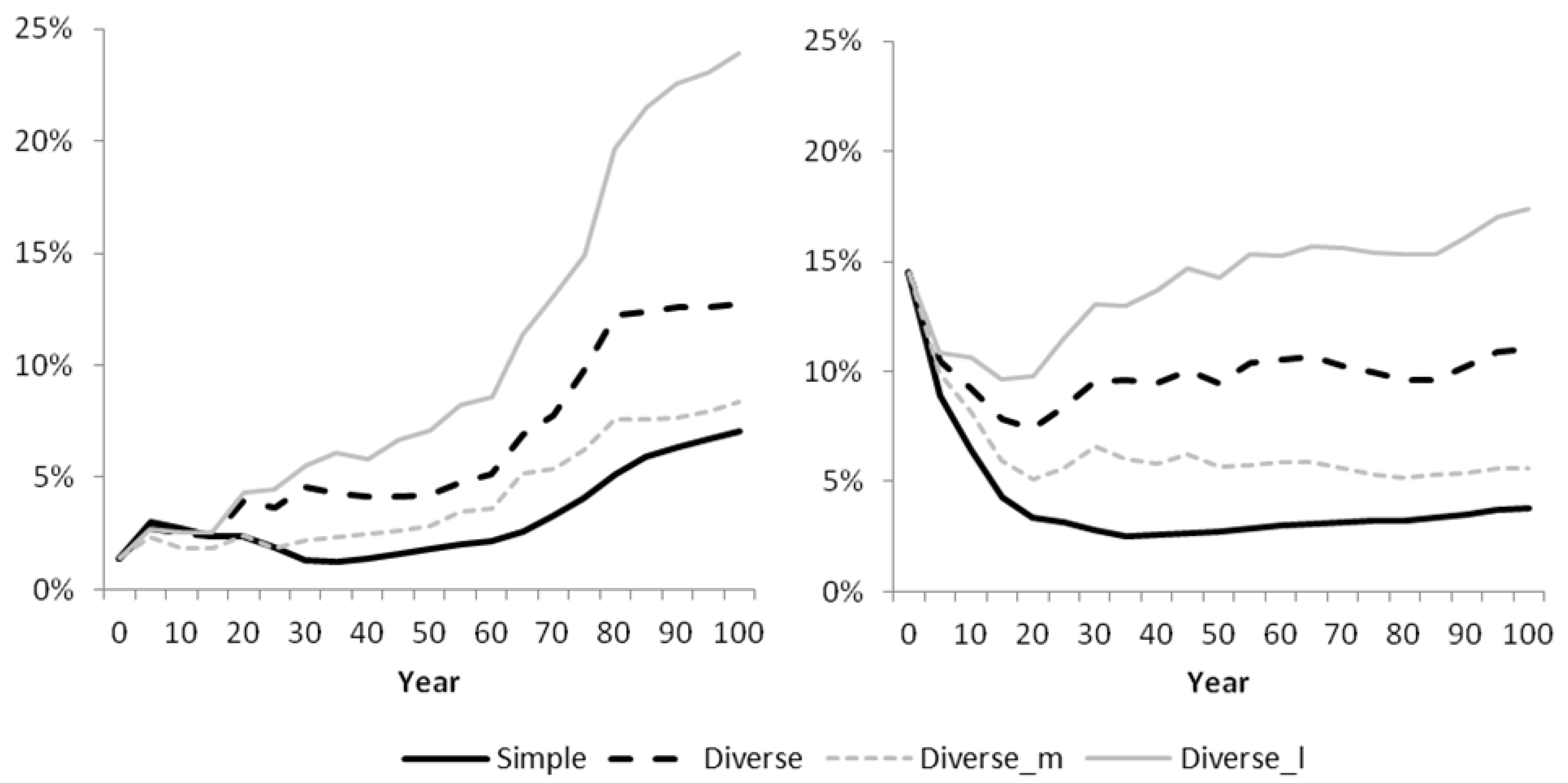
3.3.1. Sparse Forests

The proportion of sparse forest was projected to decrease considerably for both scenarios in Hässleholm during the first 50 years, from its start level of 37% (Figure 11). Even though the proportion of sparse forest increased somewhat in the latter half of the simulation period, it remained below the start level. The reduction was especially pronounced for the Simple scenario, where the proportion decreased to around 10% within only 30 years, and hardly changed thereafter. In Vilhelmina, the decrease in sparse forest was less pronounced, but even there the share almost halved over the simulation period for the Simple scenario, but remained nearly constant in the Diverse scenario (Figure 11).

Figure 11. Proportion of sparse forest in Hässleholm (left) and Vilhelmina (right) for the Simple and Diverse scenarios, as well as the more intensive (Diverse_m) and less intensive (Diverse_l) variations of the Diverse scenario. Sparse forest was defined as forest with less than 1000 stems per ha and a mean stand height of more than 10 m.

3.3.2. Clear-Cut Area

The proportion of clear-cut area was higher in the Simple scenario throughout the simulation period in both Hässleholm and Vilhelmina, with one exception in 2090 for Vilhelmina (Figure 12). The overall proportion of clear-cut area was higher in Hässleholm than in Vilhelmina, due to shorter rotation periods in southern Sweden.

Figure 12. Proportion of annual clear-cut area (excluding regeneration areas with seed or shelter tree retention) in Hässleholm (left) and Vilhelmina (right), for the Simple and Diverse scenarios, as well as the more intensive (Diverse_m) and less intensive (Diverse_l) variations of the Diverse scenario.

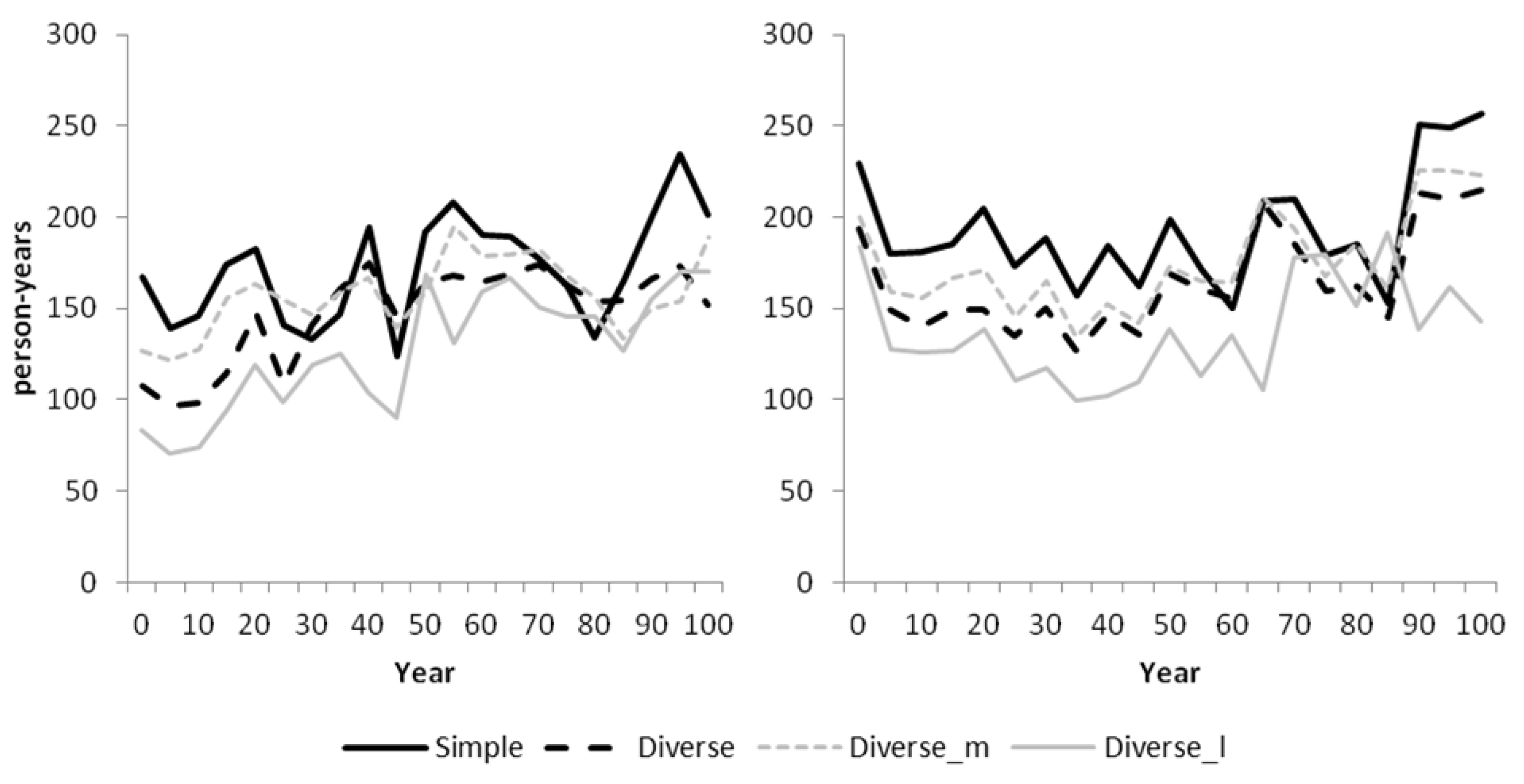
3.3.3. Person-Years

The number of person-years needed for forest management activities was higher in the Simple scenario, compared to the Diverse scenario and its alternatives (Figure 13). The majority of the working time was needed for different harvesting activities, only 5%–15% of the working time was used for soil scarification, planting and pre-commercial thinning. Therefore, the person-years reflect the development in harvest level (Figure 3) to a large degree.

Figure 13. Person-years needed for forest management activities in Hässleholm (left) and Vilhelmina (right), for the Simple and Diverse scenarios, as well as the more intensive (Diverse_m) and less intensive (Diverse_l) variations of the Diverse scenario.

3.4. Integrative Assessment

The relative medium and long-term differences between the Diverse (Diverse_m, Diverse_l) and the Simple scenario are illustrated in Table 10 (Hässleholm) and Table 11 (Vilhelmina). The medium term of 20 years corresponds to the average time of forest ownership for NIPF owners (i.e., the time between property acquisition and passing it on to the next owner) [67]. In Hässleholm (Table 10), the relative differences in scenarios were quite similar for the medium and long term. The Diverse scenario resulted in a smaller volume harvested, and thus a higher growing stock. Growth was the only indicator without relevant differences between the Diverse and Simple scenarios. In particular the ecological indicators profited from the lower felling rates in the Diverse scenario—they all increased substantially compared to the Simple scenario. Even after only 20 years of simulation, the difference between the Simple and Diverse scenarios exceeded 25% for all of the ecological indicators, with differences larger than 50% after 100 years for nearly all the ecological indicators. The effect on recreational suitability of the forests was also positive, with a higher share of sparse forests and less clear-cut area for the Diverse scenario compared to the Simple scenario. The number of person-years was somewhat lower for the Diverse scenario, due to the lower harvest level compared to the Simple scenario. The sensitivity runs revealed that some of the indicators were highly sensitive to changes in parameter settings, especially the ecological indicators, with a large difference in parameter outcome between the two sensitivity runs. However, even in the sensitivity run that was closest to the Simple scenario in indicator outcome (the Diverse_m run), most indicators were more than 10% different from the Simple scenario already after 20 years, the exceptions being growth and person-years for both time points, and the share of old forest after 20 years. The largest difference between the Simple and Diverse_m scenarios was noted for the indicator Mature forests with high share of broadleaves, with a 27% and 51% higher outcome for the Diverse_m scenario after 20 and 100 years, respectively.

Table 10. Ratio between the Diverse (Diverse_m, Diverse_l) and the Simple scenario (with Simple as reference; Simple = 1) after 20 and 100 years of simulation for Hässleholm (Simple = 1). For Total harvest, Growth and Clear-cut area, the ratio between the averages for the first and the last 20 years of simulation was used (Average 0–20 years[Diverse]/Average 0–20 years[Simple] for the first 20 years, and Average 80–100 years[Diverse]/Average 80–100 years[Simple] for the last 20 years). Differences not considered to be relevant (<10%) are presented in italics.

**Table 10.** Ratio between the Diverse (Diverse_m, Diverse_l) and the Simple scenario (with Simple as reference; Simple = 1) after 20 and 100 years of simulation for Hässleholm (Simple = 1). For Total harvest, Growth and Clear-cut area, the ratio between the averages for the first and the last 20 years of simulation was used (Average 0–20 years[Diverse]/Average 0–20 years[Simple] for the first 20 years, and Average 80–100 years[Diverse]/Average 80–100 years[Simple] for the last 20 years). Differences not considered to be relevant (<10%) are presented in italics.
Indicator	After 20 Years				After 100 Years
Indicator	Simple	Diverse	Diverse_m	Diverse_l	Diverse	Diverse_m	Diverse_l
Economic
Total harvest	1	0.71	0.85	0.51	0.86	0.82	0.84
Growing stock	1	1.28	1.18	1.45	1.23	1.17	1.45
Growth	1	1.08	1.06	1.12	0.91	0.96	0.83
Ecological
Mature forest with high share of broadleaves	1	1.48	1.27	1.74	1.57	1.51	2.09
Old forest	1	1.67	1.02	1.85	1.81	1.19	3.40
Large diameter trees	1	1.97	1.15	2.37	1.73	1.17	3.13
Fresh deadwood	1	1.26	1.15	1.48	1.44	1.16	2.03
Social
Sparse forest	1	1.54	1.30	1.88	1.94	1.83	2.76
Clear-cut area	1	0.59	0.73	0.36	0.64	0.69	0.55
Person-years	1	0.71	0.89	0.56	0.80	0.94	0.77

In Vilhelmina (Table 11), the general trends were similar as in Hässleholm. The only indicators without at least relevant (10%) differences between the scenarios were Growth and Potential reindeer winter pasture. Harvest level was lower in the Diverse scenario, resulting in a higher growing stock and a higher outcome for the ecological indicators compared to the Simple scenario, with the exception for large-diameter trees. The reason for the large difference for large-diameter trees between the scenarios was that there were very few such trees in the initial state, being present in a very small proportion (2%) of the productive forest area in the initial state, resulting in less than 0.5 trees per ha (compare Figure 9), so that even small differences in harvest location and volume in the first few years can have a great effect. Also in Vilhelmina, the recreational suitability of forests was increased in the Diverse scenario by a higher share of sparse forest and a lower share of clear-cut areas compared to the Simple scenario. As in Hässleholm, the sensitivity runs revealed that indicator outcomes were sensitive to parameter settings to some extent, especially for the Old forest indicator. However, even in Vilhelmina, the difference between the Diverse_m and the Simple scenarios exceeded 10% for most indicators at both time points, with the exception of Growing stock, Growth and Potential reindeer winter pasture after 20 years, and Total harvest and Growth after 100 years. The largest difference between the Diverse_m and the Simple scenarios was found for the Old forest indicator, with an approximately 50% higher outcome for the Diverse_m scenario at both time points.

Table 11. Ratio between the Diverse (Diverse_m, Diverse_l) and the Simple scenario (with Simple as reference; Simple = 1) after 20 and 100 years of simulation for Vilhelmina (Simple = 1). For Total harvest, Growth and Clear-cut area, the ratio between the averages for the first and the last 20 years of simulation was used (Average 0–20 years [Diverse]/Average 0–20 years[Simple] for the first 20 years, and Average 80–100 years [Diverse]/Average 80–100 years[Simple] for the last 20 years). Differences not considered to be relevant (<10%) are presented in italics.

**Table 11.** Ratio between the Diverse (Diverse_m, Diverse_l) and the Simple scenario (with Simple as reference; Simple = 1) after 20 and 100 years of simulation for Vilhelmina (Simple = 1). For Total harvest, Growth and Clear-cut area, the ratio between the averages for the first and the last 20 years of simulation was used (Average 0–20 years [Diverse]/Average 0–20 years[Simple] for the first 20 years, and Average 80–100 years [Diverse]/Average 80–100 years[Simple] for the last 20 years). Differences not considered to be relevant (<10%) are presented in italics.
Indicator		After 20 Years			After 100 Years
Indicator	Simple	Diverse	Diverse_m	Diverse_l	Diverse	Diverse_m	Diverse_l
Economic
Total harvest	1	0.78	0.88	0.68	0.88	0.95	0.72
Growing stock	1	1.14	1.09	1.20	1.37	1.27	1.58
Growth	1	1.04	1.04	1.05	1.01	1.05	0.92
Potential reindeer winter pasture	1	0.94	0.95	0.96	0.92	0.85	1.08
Ecological
Mature forest with high share of broadleaves (%)	1	1.29	1.14	1.47	1.29	1.18	1.43
Old forest	1	2.22	1.53	2.94	2.89	1.47	4.55
Large diameter trees	1	0.32	0.38	6.28	1.01	1.44	2.75
Fresh deadwood	1	1.25	1.16	1.36	1.55	1.44	1.91
Social
Sparse forest	1	1.23	1.16	1.46	1.84	1.41	2.82
Clear-cut area	1	0.69	0.79	0.56	0.74	0.80	0.60
Person-years	1	0.78	0.87	0.69	0.86	0.92	0.70

In summary, the observed differences in indicator outcome in both municipalities show that decreasing harvest volume leads to a higher outcome for the biodiversity-related indicators as well as higher recreational suitability, and thus indicate a trade-off between wood production on the one hand, and biodiversity and recreation on the other hand.

3.5. Differences by Forest Owner Category

In Hässleholm, the difference in harvest level between the Diverse and Simple scenarios was larger for NIPF owners compared to other owners (Table 12), which in turn resulted in larger differences in growing stock, ecological and social indicators, both in the medium (20 years) and long term (100 years). Differences between the scenarios were relevant for all indicators except growth already in the medium term of 20 years. Also in Vilhelmina, there were relevant differences between the scenarios already after 20 years of simulation (Table 13), with the exception of Growth and Potential reindeer winter pasture. However, the relative difference in indicator values after 20 years was quite similar for the two ownership categories (Table 13). This is due to the fact that both the NIPF and the other owner categories include owner types with rather low-intensity management strategies (the passive NIPF owners and the forest commons as well as the National Property Board), which decrease harvest levels for both categories compared to the Simple scenario.

Table 12. Differences between the Diverse and Simple scenarios for economic, ecological and social indicators after 20 and 100 years of simulation, by ownership category, in Hässleholm. The relative differences (Rel. ∆) were calculated as: (Diverse-Simple)/Simple. See Table 2 for information on the proportion of different owner categories.

**Table 12.** Differences between the Diverse and Simple scenarios for economic, ecological and social indicators after 20 and 100 years of simulation, by ownership category, in Hässleholm. The relative differences (Rel. ∆) were calculated as: (Diverse-Simple)/Simple. See Table 2 for information on the proportion of different owner categories.
Owner Type	Non-Industrial Private Owners						Other Owners
	After 20 Years			After 100 Years			After 20 Years			After 100 Years
	Simple	Diverse	Rel. ∆	Simple	Diverse	Rel. ∆	Simple	Diverse	Rel. ∆	Simple	Diverse	Rel. ∆
Economic indicators
Total harvest (1000 m³/year) *	371	259	−0.30	519	433	−0.16	53	42	−0.19	63	65	0.03
Growing stock (m³/ha)	177	229	0.30	282	361	0.28	206	241	0.17	347	343	−0.01
Growth (m³/ha/year) *	7.1	7.7	0.08	8.7	7.9	−0.10	7.4	7.8	0.05	8.1	8.0	−0.02
Ecological indicators
Mature forest with high share of broadleaves (%)	20	37	0.81	21	35	0.65	29	39	0.34	28	33	0.17
Old forest (%)	2	4	0.74	6	13	1.15	3	5	0.39	14	12	−0.13
Large diameter trees (trees/ha)	6.4	13.2	1.05	11.3	22.2	0.97	8.7	13.8	0.6	25.7	26.9	0.05
Fresh deadwood (m³/ha)	7.9	10.1	0.29	15.8	24.7	0.56	9.73	11.2	0.1	23.7	21.4	−0.10
Social indicators
Sparse forest (%)	17	27	0.57	10	21	1.05	22	31	0.40	14	20	0.44
Clear-cut area (%) *	1.3	0.8	−0.42	1.2	0.8	−0.37	1.2	0.8	−0.34	1.0	0.7	−0.24
Person-years (years) *	140	98	−0.30	178	139	−0.22	21	16	−0.21	22	22	0.00

* Average for first and last 20 years of simulation (1–20 and 81–100 years), respectively, for indicators without initial value in the input data.

Table 13. Differences between the Diverse and Simple scenarios for economic, ecological and social indicators after 20 and 100 years of simulation, by ownership category, in Vilhelmina. The relative difference (Rel. ∆) was calculated as: (Diverse-Simple)/Simple. See Table 2 for information on the proportion of different owner categories.

**Table 13.** Differences between the Diverse and Simple scenarios for economic, ecological and social indicators after 20 and 100 years of simulation, by ownership category, in Vilhelmina. The relative difference (Rel. ∆) was calculated as: (Diverse-Simple)/Simple. See Table 2 for information on the proportion of different owner categories.
Owner Type	Non-Industrial Private Owners						Other Owners
	After 20 Years			After 100 Years			After 20 Years			After 100 Years
	Simple	Diverse	Rel. ∆	Simple	Diverse	Rel. ∆	Simple	Diverse	Rel. ∆	Simple	Diverse	Rel. ∆
Economic indicators
Total harvest (1000 m³/year) *	276	210	−0.24	345	277	−0.20	340	273	−0.20	440	417	−0.05
Growing stock (m³/ha)	84	95	0.14	139	202	0.45	82	92	0.13	144	187	0.30
Growth (m³/ha/year) *	2.2	2.4	0.06	3.3	3.4	0.02	2.4	2.4	0.03	3.4	3.3	−0.01
Potential reindeer winter pasture (%)	7	7	0.01	4	3	−0.33	12	11	−0.09	3	4	0.18
Ecological indicators
Mature forest with high share of broadleaves (%)	19	24	0.23	23	32	0.42	14	15	0.06	26	31	0.19
Old forest (%)	4	8	0.88	4	10	1.35	2	7	1.71	3	12	2.49
Large diameter trees (trees/ha)	0.1	0.0	−0.64	0.7	1.6	1.32	0.0	0.0	−0.5	0.7	1.3	0.73
Fresh deadwood (m³/ha)	4.64	5.64	0.22	7.86	12.33	0.57	3.83	4.91	0.28	7.49	11.45	0.53
Social indicators
Sparse forest (%)	14	16	0.20	10	20	0.89	12	15	0.24	9	16	0.79
Clear-cut area (%) *	1.0	0.7	−0.31	0.7	0.4	−0.38	1.1	0.7	−0.31	0.7	0.6	−0.15
Person-years (years) *	83	64	−0.23	101	79	−0.22	105	83	−0.21	126	117	−0.08

* Average for first and last 20 years of simulation (1–20 and 81–100 years), respectively, for indicators without initial value in the input data.4. Discussion

4. Discussion

Our results demonstrate marked differences between the modeled outcomes for a Diverse scenario, taking into account the diversity in management strategies of different forest owners and within owner categories, and a Simple scenario, where forest owners were aggregated into two broad categories with similar management strategies. The differences between the scenarios were most pronounced for the ecological and, to some extent, the social indicators, indicating that moderate decreases in harvest level can have a considerable positive effect on forest’s biodiversity and recreational value. The differences between the two scenarios were quite similar in both case study areas, despite the differences in growing conditions and ownership structure between the two municipalities, indicating a broader applicability of our results. The Simple scenario was based on the reference scenario of the Swedish forest impact analysis study [2], and can be understood as a maximum sustainable yield scenario with some legal and environmental considerations, while the Diverse scenario added constraints put in place by a diverse ownership structure. Our results thus suggest that generalizing forest management for forest owner categories can lead to considerable over- or underestimation of ecosystem service provision in forest resource projections when the diversity of management strategies between and within owner categories is not accounted for. In contrast to technical and environmental constraints affecting forest management, social constraints are rarely taken into account in projections of forest resource development and wood mobilization scenarios [68], even though it has been shown that social constraints could have an important impact on future wood supply and forest development [4,12,16,19]. When the results of forest impact analysis are used as the basis for decision-making regarding the long-term use of forests, as is the case in Sweden, it is important that all relevant constraints within forest management are considered.

Growing stock increased considerably in both case study areas and in both scenarios. In Hässleholm, after 100 years, growing stock was projected to equal (Simple scenario) or exceed (Diverse scenario) the current growing stock of central European countries with nemoral forest, such as Germany and Austria, where the standing volume is currently around 300 m³/ha [51]. Mean volume in Vilhelmina reached or exceeded the current mean volume typical for forests in southern Sweden today within 100 years. This is, in part, a consequence of an increasing proportion of old forest and mean age, especially in the Diverse scenario, and, in part, due to the projected increasing growth especially in 40–80 year-old forests (40–100 years in Vilhelmina), leading to higher mean volumes in middle-aged and mature forests over time. Similarly, Pussinen et al. [7] found increasing standing volumes in mid- and high latitude European forests, even though the increase was not as pronounced as in our study; this could, in part, be due to the fact that the model used by Pussinen et al. did not include effects of tree breeding and fertilization, and was based on conservative growth functions. Higher growing stocks due to increased growth allow for an increasing harvest level, as seen in our results, but they also require considerations about the timing and intensity of silvicultural activities such as thinnings and final fellings, and potential disturbance risk. While natural mortality was included in modeling of forest growth, disturbances were not included in our simulations. Disturbances could, however, have a considerable effect on forests locally and regionally, as illustrated by catastrophic storm events in the past, e.g., the 2005 winter hurricane in Sweden, which led to storm-felling amounting to almost the total annual harvest in Sweden, damaging more than 1% of the productive forest area [69]. The susceptibility of forests to devastating disturbance events increases as the proportion of old and densely-stocked forests increases, especially in conifer monocultures [70]. It is possible that forest management strategies change over time to some extent due to changed risk perceptions [71]. This was, however, outside the scope of this study.

The management strategies employed in this study are subjective to some degree, as not all parameters are backed up by sufficient data. This is especially the case for the management strategies of NIPF owners, which were based on a questionnaire and the forest owners’ own perceptions of how they manage their forest. During recent years, research has focused on the difference in objectives, attitudes and decision-making style of NIPF owners in Sweden and elsewhere, not on actual management practices, resulting in a lack of quantitative data allowing the classification of NIPF owners according to their management strategy [25]. Therefore, we conducted a sensitivity analysis (Diverse_m and Diverse_l) to test for the impact of subjectivity in parameter settings for NIPF owners’ management strategies. The sensitivity analysis should not be regarded as estimates of standard errors or confidence intervals or similar, but rather as alternative interpretations of the management strategies of NIPF owners. We found that the results were sensitive to parameter settings to some extent, but a difference exceeding 10% remained between the Simple scenario and the sensitivity run alternative of the Diverse scenario that was closest to the Simple scenario, for most of the indicators. Nevertheless, the changes in the Diverse scenario settings, simulating more and less intensive forest management respectively, resulted in quite different developments for some of the investigated indicators, especially for the ecological indicators. This highlights the need for further and deeper investigations of the management behavior of different types of forest owners, especially since it is suspected that such behavioral patterns change over time.

The accuracy of long-term projections of forest development quite naturally depends heavily on the growth models used. In tests on NFI data and long-term research plot data, the Heureka growth models have been shown to be quite reliable for even-aged management given there are no catastrophic events such as fire or storm [40]. They have performed less accurately in tests on heterogeneously structured forest [72], for which growth in long-term projections also depends on the natural ingrowth of trees [41]. The growth models have also been shown to be reasonably accurate for projecting growth of non-managed old growth forests [73].

As in all modeling, the quality of the input data determines the quality of the results. Our input data were based on a combination of satellite data and field data from NFI. Satellite data estimates on pixel level have a high Root Mean Square Error (RMSE) and a low bias. The estimates tend to be more accurate toward the mean value, with underestimations of higher values and overestimations of lower values. At a stand level, RMSE for the volume estimations was about 33% in southwestern Sweden in similar conditions as in Hässleholm [31]. In another study the RMSE ranged from 39% to 17% at stand level, and was down to 10% for a 100 ha assessment [74]. As the accuracy over larger areas is fairly good, the quality of the input data should not influence the results and conclusions of the study. Having input data from different time periods for the two municipalities is not expected to influence the results or conclusions either, given the long rotation periods in Swedish forests and the scope of our study.

We did not include the potential impact of climate change in our analysis, as the focus of this study was on demonstrating a method for and the impacts of accounting for diverse forest ownership structure, i.e., on relative differences between two different management scenarios. Expected climate change impacts in Sweden include warmer temperatures, especially in winter, and an increase in precipitation. The warmer climate and increased atmospheric CO₂ levels are expected to increase tree growth and wood production [75], except at water-limited sites in southern Sweden. Biotic and abiotic disturbance risks are also expected to change. However, there remains considerable uncertainty regarding the future trajectories of greenhouse gas increases, their impact on the climate system and the effects of climatic changes on both ecosystems and social systems and their adaptive capacity [75,76,77]. For this study, we assumed that climate change would have similar impacts on both scenarios, so that including potential climate change impacts would not add new valuable insights to the comparison of the scenarios.

In our analysis, we assumed that the relative level of use of different management strategies would remain constant over time and that forest stands would remain under one management strategy for the whole simulation period. However, in reality, private forest properties change owners approximately every 20 years, and with a new owner, the management strategy might also change. Implementing the effect of ownership changes could be an area of future development of the methodology.

5. Conclusions

This paper reports on a method to quantify the potential effect of accounting for heterogeneity in forest management strategies among and within ownership categories in projections of forest sustainability indicators. The impact of accounting for differences in management strategies between and within different forest owner groups was examined by comparing two scenarios—one where the diversity of management strategies was accounted for and one where it was not—for two municipalities in Sweden. We found marked differences in the outcomes for the two scenarios, especially for ecological indicators, and we expect that similar differences would be found for other regions in Sweden. The method we employed could be easily adapted for other regions, and even for larger areas. The modeling framework could provide valuable information for municipality planning, for follow-up and planning for attempts to reach environmental and other objectives related to forests, but it could also be employed at a larger (up to national) scale, given the availability of sufficient input data for the current forest state and the management strategies of different owner groups. We conclude that the diversity in management strategies between and within owner categories deserves more attention in future projections of wood supply and forest ecosystem services. Establishing a better understanding of different ownership categories and their inherent management strategies in quantitative terms would be very valuable for future modeling activities at regional to national scale.

Acknowledgments

This research was performed within the PLURAL project (Planning for Rural-Urban Dynamics: Living and Acting at Several Places) and funded by the Swedish Research Council Formas. We thank Dr. Anu Korosuo for helping with the input data preparation, and Anders Lundström for his comments. We are grateful for the valuable comments of two anonymous reviewers, which helped improve the manuscript.

Author Contributions

All authors contributed to the study design. Jeannette Eggers prepared most of the input data, conducted the model analysis and prepared the manuscript. All authors contributed to the manuscript revisions.

Conflicts of Interest

The authors declare no conflict of interest.

References

Mantau, U.; Saal, U.; Prins, K.; Steierer, F.; Lindner, M.; Verkerk, H.; Eggers, J.; Leek, N.; Oldenburger, J.; Asikainen, A.; et al. EUwood—Real Potential for Changes in Growth and Use of EU Forest. Final Report; University of Hamburg (Centre of Wood Science) (UHAM): Hamburg, Germany, 2010; p. 160. [Google Scholar]
Claesson, S. Skogsstyrelsen Skogliga Konsekvensanalyser 2008-SKA-VB 08; Skogsstyrelsen: Jönköping, Sweden, 2008; p. 157. [Google Scholar]
UNECE/FAO. The European Forest Sector Outlook Study II. 2010–2030; United Nations: Geneva, Switzerland, 2011. [Google Scholar]
Verkerk, P.J.; Anttila, P.; Eggers, J.; Lindner, M.; Asikainen, A. The realisable potential supply of woody biomass from forests in the European Union. For. Ecol. Manag. 2011, 261, 2007–2015. [Google Scholar] [CrossRef]
Eggers, J.; Lindner, M.; Zudin, S.; Zaehle, S.; Liski, J. Impact of changing wood demand, climate and land use on European forest resources and carbon stocks during the 21st century. Glob. Chang. Biol. 2008, 14, 2288–2303. [Google Scholar] [CrossRef]
Verkerk, P.J.; Mavsar, R.; Giergiczny, M.; Lindner, M.; Edwards, D.; Schelhaas, M.J. Assessing impacts of intensified biomass production and biodiversity protection on ecosystem services provided by European forests. Ecosyst. Serv. 2014, 9, 155–165. [Google Scholar] [CrossRef]
Pussinen, A.; Nabuurs, G.J.; Wieggers, H.J.J.; Reinds, G.J.; Wamelink, G.W.W.; Kros, J.; Mol-Dijkstra, J.P.; de Vries, W. Modelling long-term impacts of environmental change on mid- and high-latitude European forests and options for adaptive forest management. For. Ecol. Manag. 2009, 258, 1806–1813. [Google Scholar] [CrossRef]
Hengeveld, G.M.; Didion, M.; Clerkx, S.; Elkin, C.; Nabuurs, G.-J.; Schelhaas, M.-J. The landscape-level effect of individual-owner adaptation to climate change in Dutch forests. Reg. Environ. Chang. 2014. [Google Scholar] [CrossRef]
Frank, S.; Fürst, C.; Pietzsch, F. Cross-Sectoral Resource Management: How Forest Management Alternatives Affect the Provision of Biomass and Other Ecosystem Services. Forests 2015, 6, 533–560. [Google Scholar] [CrossRef]
Dunbar, M.B.; Panagos, P.; Montanarella, L. European perspective of ecosystem services and related policies. Integr. Environ. Assess. Manag. 2013, 9, 231–236. [Google Scholar] [CrossRef] [PubMed]
Egoh, B.; Dunbar, M.B.; Maes, J.; Willemen, L.; Drakou, E.G.; European Commission; Joint Research Centre; Institute for Environment and Sustainability. Indicators for Mapping Ecosystem Services: A Review; Publications Office: Luxembourg, Luxembourg, 2012. [Google Scholar]
Antón-Fernández, C.; Astrup, R. Empirical harvest models and their use in regional business-as-usual scenarios of timber supply and carbon stock development. Scand. J. For. Res. 2012, 27, 379–392. [Google Scholar] [CrossRef]
Eid, T. Testing a large-scale forestry scenario model by means of successive inventories on a forest property. 2004, 38, 305–317. [Google Scholar]
Boon, T.E.; Meilby, H.; Thorsen, B.J. An Empirically Based Typology of Private Forest Owners in Denmark: Improving Communication between Authorities and Owners. Scand. J. For. Res. 2004, 19, 45–55. [Google Scholar] [CrossRef]
Ingemarson, F.; Lindhagen, A.; Eriksson, L. A typology of small-scale private forest owners in Sweden. Scand. J. For. Res. 2006, 21, 249–259. [Google Scholar] [CrossRef]
Schaich, H.; Plieninger, T. Land ownership drives stand structure and carbon storage of deciduous temperate forests. For. Ecol. Manag. 2013, 305, 146–157. [Google Scholar] [CrossRef]
Rinaldi, F.; Jonsson, R.; Sallnäs, O.; Trubins, R. Behavioral Modelling in a Decision Support System. Forests 2015, 6, 311–327. [Google Scholar] [CrossRef]
Arano, K.G.; Munn, I.A. Evaluating forest management intensity: A comparison among major forest landowner types. For. Policy Econ. 2006, 9, 237–248. [Google Scholar] [CrossRef]
Johnson, K.N.; Bettinger, P.; Kline, J.D.; Spies, T.A.; Lennette, M.; Lettman, G.; Garber-Yonts, B.; Larsen, T. Simulation forest structure, timber production, and socioeconomic effects in a multi-owner province. Ecol. Appl. 2007, 17, 34–47. [Google Scholar] [CrossRef]
Zheng, D.L.; Heath, L.S.; Ducey, M.J.; Butler, B. Relationships Between Major Ownerships, Forest Aboveground Biomass Distributions, and Landscape Dynamics in the New England Region of USA. Environ. Manag. 2010, 45, 377–386. [Google Scholar] [CrossRef] [PubMed]
Swedish Forest Agency. Swedish Statistical Yearbook of Forestry 2013; Skogsstyrelsen: Jönköping, Sweden, 2013. [Google Scholar]
Simonsson, P.; Gustafsson, L.; Östlund, L. Retention forestry in Sweden: Driving forces, debate and implementation 1968–2003. Scand. J. For. Res. 2015, 30, 154–173. [Google Scholar] [CrossRef]
Naturvårdsverket. Miljömålen. Årlig Uppföljning av Sveriges Miljökvalitetsmål och Etappmål 2014; Naturvårdsverket: Stockholm, Sverige, 2014; p. 306. [Google Scholar]
Zaremba, M. Skogen vi Ärvde; Weyler: Stockholm, Sverige, 2012. [Google Scholar]
Eggers, J.; Lämås, T.; Lind, T.; Öhman, K. Factors Influencing the Choice of Management Strategy among Small-Scale Private Forest Owners in Sweden. Forests 2014, 5, 1695–1716. [Google Scholar] [CrossRef]
Gustafsson, K.; Hägg, S. Skogliga Konsekvensanalyser 2003 SKA 03; Skogsstyrelsen: Jönköping, Sweden, 2004; p. 52. [Google Scholar]
SCB Area by Municipality 1 January 2015 (km²). Available online: http://www.scb.se/sv_/Hitta-statistik/Statistik-efter-amne/Miljo/Markanvandning/Land--och-vattenarealer/12838/12845/ (accessed on 24 September 2015).
SCB Befolkningsstatistik. Available online: http://www.scb.se/be0101/ (accessed on 24 September 2015).
EEA Biogeographical Regions. Available online: http://www.eea.europa.eu/data-and-maps/data/biogeographical-regions-europe-2 (accessed on 24 September 2015).
SMHI Vegetationsperiodens längd. Available online: http://www.smhi.se/klimatdata/meteorologi/temperatur/vegetationsperiodens-langd-1.4076 (accessed on 23 September 2015).
Reese, H.; Nilsson, M.; Pahén, T.G.; Hagner, O.; Joyce, S.; Tingelöf, U.; Egberth, M.; Olsson, H. Countrywide estimates of forest variables using satellite data and field data from the National Forest Inventory. Ambio 2003, 32, 542–548. [Google Scholar] [CrossRef] [PubMed]
Fridman, J.; Ståhl, G. A Three-step Approach for Modelling Tree Mortality in Swedish Forests. Scand. J. For. Res. 2001, 16, 455–466. [Google Scholar] [CrossRef]
Metria Markägarkartan (Ownership map). Available online: http://www.metria.se/Vara-erbjudanden/Kartor-och-bilder/Metria-som-geodataleverantor/Fastighetskartor/Markagarkartan/ (accessed on 2 September 2014).
Skogsstyrelsen. Öppna data—Skogsstyrelsen. Available online: http://www.skogsstyrelsen.se/Myndigheten/Om-oss/Oppna-data/ (accessed on 27 May 2015).
Skogsstyrelsen. Skogsdataportalen. Available online: http://skogsdataportalen.skogsstyrelsen.se/Skogsdataportalen/ (accessed on 25 September 2015).
Naturvårdsverket. Naturvårdsverkets nedladdningstjänst för geodata. Available online: http://data.naturvardsverket.se/DataSet/Details/5 (accessed on 25 September 2015).
Nilsson, H. Strategic Forest Planning Using AHP and TOPSIS in Participatory Environments. A Case Study Conducted in Wilhelmina, Sweden. Master’s Thesis, Swedish University of Agricultural Sciences (SLU), Umeå, Sweden, 2014. [Google Scholar]
Statens Fastighetsverk Google Earth—Statens fastighetsverk. Available online: http://www.sfv.se/sv/fastigheter/skogar-och-marker/google-earth/ (accessed on 27 May 2015).
Wikström, P.; Edenius, L.; Elfving, B.; Eriksson, L.O.; Lämås, T.; Sonesson, J.; Öhman, K.; Wallerman, J.; Waller, C.; Klintebäck, F. The Heureka Forestry Decision Support System: An Overview. Math. Comput. For. Nat.-Resour. Sci. 2011, 3, 87–95. [Google Scholar]
Fahlvik, N.; Elfving, B.; Wikström, P. Evaluation of growth functions used in the Swedish Forest Planning System Heureka. Silva Fenn. 2014, 48. [Google Scholar] [CrossRef]
Wikberg, P.-E. Occurrence, morphology and growth of understory saplings in Swedish forests. Available online: http://pub.epsilon.slu.se/610/ (accessed on 26 May 2015).
Holm, S.; Lundström, A. Åtgärdsprioriteter (Management Priorities); SLU: Umeå, Sweden, 2000; p. 17. [Google Scholar]
Södra. Virkesprislista—Södra. Available online: http://skog.sodra.com/sv/Salja-Virke/Virkesprislista/ (accessed on 26 March 2015).
Norra Skogsägarna Prislistor—Norra Skogsägarna. Available online: http://www.norra.se/verksamhet/skogochvirke/Saljavirke/Sidor/prislistor.aspx (accessed on 11 February 2015).
Brunberg, T. Underlag för Produktionsnorm för Engreppsskördare i Gallring (Basic Data for Productivity Norms for Single-Grip Harvesters in Thinning); Redogörelse nr 8; SkogForsk: Uppsala, Sweden, 1997. [Google Scholar]
Brunberg, T. Underlag för Produktionsnorm för Stora Engreppsskördare i Slutavverkning (Basic data for productivity Norms for Heavy-Duty Single-Grip Harvesters in final Felling); Redogörelse nr 7; SkogForsk: Uppsala, Sweden, 1995. [Google Scholar]
Brunberg, T. Underlag till produktionsnormer för skotare (Productivity-Norm Data for Forwarders); Redogörelse nr 3; Skogforsk: Uppsala, Sweden, 2004. [Google Scholar]
Lämås, T.; Sandström, E.; Jonzén, J.; Olsson, H.; Gustafsson, L. Tree retention practices in boreal forests—What kind of future landscapes are we creating? Scand. J. For. Res. 2015, 30, 526–537. [Google Scholar] [CrossRef]
Bettinger, P.; Boston, K.; Siry, J.P.; Grebner, D.L. Forest Management and Planning; Academic Press: Waltham, MA, USA, 2009. [Google Scholar]
Biber, P.; Borges, J.G.; Moshammer, R.; Barreiro, S.; Botequim, B.; Brodrechtová, Y.; Brukas, V.; Chirici, G.; Cordero-Debets, R.; Corrigan, E.; et al. How Sensitive Are Ecosystem Services in European Forest Landscapes to Silvicultural Treatment? Forests 2015, 6, 1666–1695. [Google Scholar] [CrossRef]
Forest Europe; UNECE; FAO. State of Europe’s Forests 2011. Status and Trends in Sustainable Forest Management in Europe; United Nations: Geneva, Switzerland, 2011. [Google Scholar]
Petersson, H.; Holm, S.; Ståhl, G.; Alger, D.; Fridman, J.; Lehtonen, A.; Lundström, A.; Mäkipää, R. Individual tree biomass equations or biomass expansion factors for assessment of carbon stock changes in living biomass—A comparative study. For. Ecol. Manag. 2012, 270, 78–84. [Google Scholar] [CrossRef]
Triviño, M.; Juutinen, A.; Mazziotta, A.; Miettinen, K.; Podkopaev, D.; Reunanen, P.; Mönkkönen, M. Managing a boreal forest landscape for providing timber, storing and sequestering carbon. Ecosyst. Serv. 2015, 14, 179–189. [Google Scholar] [CrossRef]
Korosuo, A.; Sandström, P.; Öhman, K.; Eriksson, L.O. Impacts of different forest management scenarios on forestry and reindeer husbandry. Scand. J. For. Res. 2014, 29, 234–251. [Google Scholar] [CrossRef]
Nilsson, S.G.; Hedin, J.; Niklasson, M. Biodiversity and its assessment in boreal and nemoral forests. Scand. J. For. Res. 2001, 16, 10–26. [Google Scholar] [CrossRef]
Roberge, J.-M.; Lämås, T.; Lundmark, T.; Ranius, T.; Felton, A.; Nordin, A. Relative contributions of set-asides and tree retention to the long-term availability of key forest biodiversity structures at the landscape scale. J. Environ. Manag. 2015, 154, 284–292. [Google Scholar] [CrossRef] [PubMed]
Gustafsson, L. Presence and Abundance of Red-Listed Plant Species in Swedish Forests. Conserv. Biol. 2002, 16, 377–388. [Google Scholar] [CrossRef]
Liira, J.; Kohv, K. Stand characteristics and biodiversity indicators along the productivity gradient in boreal forests: Defining a critical set of indicators for the monitoring of habitat nature quality. Plant Biosyst. Int. J. Deal. Asp. Plant Biol. 2010, 144, 211–220. [Google Scholar] [CrossRef]
Lundström, J.; Öhman, K.; Perhans, K.; Rönnqvist, M.; Gustafsson, L.; Bugman, H. Cost-effective age structure and geographical distribution of boreal forest reserves. J. Appl. Ecol. 2011, 48, 133–142. [Google Scholar] [CrossRef] [PubMed]
Lassauce, A.; Paillet, Y.; Jactel, H.; Bouget, C. Deadwood as a surrogate for forest biodiversity: Meta-analysis of correlations between deadwood volume and species richness of saproxylic organisms. Ecol. Indic. 2011, 11, 1027–1039. [Google Scholar] [CrossRef]
Djupström, L. Conservation of Saproxylic species an Evaluation of Set-Asides and Substrates in Boreal Forests; Dept. of Ecology, Swedish University of Agricultural Sciences: Uppsala, Sweden, 2010. [Google Scholar]
Nordström, E.-M.; Holmström, H.; Öhman, K. Evaluating continuous cover forestry based on the forest owner’s objectives by combining scenario analysis and multiple criteria decision analysis. Silva Fenn. 2013, 47. [Google Scholar] [CrossRef]
Gundersen, V.S.; Frivold, L.H. Public preferences for forest structures: A review of quantitative surveys from Finland, Norway and Sweden. Urban For. Urban Green 2008, 7, 241–258. [Google Scholar] [CrossRef]
Fredman, P.; Stenseke, M.; Sandell, K.; Mossing, A. Friluftsliv i Förändring; Naturvårdsverket: Stockholm, Sverige, 2013. [Google Scholar]
Fredman, P.; Margaryan, L. The Supply of Nature-based Tourism in Sweden : A National Inventory of Service Providers; European Tourism Research Institute: Mittuniversitetet, Sweden, 2014. [Google Scholar]
NFI. Fältinstruktion 2014, Riksinventeringen av Skog; SLU: Umeå, Sweden, 2014; p. 470. [Google Scholar]
Eriksson, L. Åtgärdsbeslut i Privatskogsbruket (Treatment Decisions in Privately Owned Forestry); SLU: Uppsala, Sweden, 2008. [Google Scholar]
Eyvindson, K.; Kangas, A. Using a Compromise Programming Framework to Integrating Spatially Specific Preference Information for Forest Management Problems. J. Multi-Criteria Decis. Anal. 2015, 22, 3–15. [Google Scholar] [CrossRef]
Lidskog, R.; Sjödin, D. Why do forest owners fail to heed warnings? Conflicting risk evaluations made by the Swedish forest agency and forest owners. Scand. J. For. Res. 2014, 29, 275–282. [Google Scholar] [CrossRef]
Seidl, R.; Schelhaas, M.-J.; Lexer, M.J. Unraveling the drivers of intensifying forest disturbance regimes in Europe. Glob. Chang. Biol. 2011, 17, 2842–2852. [Google Scholar] [CrossRef]
Blennow, K. Adaptation of forest management to climate change among private individual forest owners in Sweden. For. Policy Econ. 2012, 24, 41–47. [Google Scholar] [CrossRef]
Drössler, L.; Fahlvik, N.; Elfving, B. Application and limitations of growth models for silvicultural purposes in heterogeneously structured forest in Sweden. J. For. Sci. 2013, 59, 458–473. [Google Scholar]
Elfving, B.; Wikberg, P.-E. Jämförelse av Observerad och Med Heureka Beräknad Utveckling på Urskogsytorna (Comparison of Observed and Heureka-Simulated Development of Primeval Forest Areas), Unpublished work. 2015.
Reese, H.; Nilsson, M.; Sandström, P.; Olsson, H. Applications using estimates of forest parameters derived from satellite and forest inventory data. Comput. Electron. Agric. 2002, 37, 37–55. [Google Scholar] [CrossRef]
Lindner, M.; Maroschek, M.; Netherer, S.; Kremer, A.; Barbati, A.; Garcia-Gonzalo, J.; Seidl, R.; Delzon, S.; Corona, P.; Kolström, M.; et al. Climate change impacts, adaptive capacity, and vulnerability of European forest ecosystems. For. Ecol. Manag. 2010, 259, 698–709. [Google Scholar] [CrossRef]
Keenan, R.J. Climate change impacts and adaptation in forest management: A review. Ann. For. Sci. 2015, 72, 145–167. [Google Scholar] [CrossRef]
Wilby, R.L.; Dessai, S. Robust adaptation to climate change. Weather 2010, 65, 180–185. [Google Scholar] [CrossRef]

© 2015 by the authors; licensee MDPI, Basel, Switzerland. This article is an open access article distributed under the terms and conditions of the Creative Commons Attribution license (http://creativecommons.org/licenses/by/4.0/).

Share and Cite

MDPI and ACS Style

Eggers, J.; Holmström, H.; Lämås, T.; Lind, T.; Öhman, K. Accounting for a Diverse Forest Ownership Structure in Projections of Forest Sustainability Indicators. Forests 2015, 6, 4001-4033. https://doi.org/10.3390/f6114001

AMA Style

Eggers J, Holmström H, Lämås T, Lind T, Öhman K. Accounting for a Diverse Forest Ownership Structure in Projections of Forest Sustainability Indicators. Forests. 2015; 6(11):4001-4033. https://doi.org/10.3390/f6114001

Chicago/Turabian Style

Eggers, Jeannette, Hampus Holmström, Tomas Lämås, Torgny Lind, and Karin Öhman. 2015. "Accounting for a Diverse Forest Ownership Structure in Projections of Forest Sustainability Indicators" Forests 6, no. 11: 4001-4033. https://doi.org/10.3390/f6114001

Article Menu

Accounting for a Diverse Forest Ownership Structure in Projections of Forest Sustainability Indicators

Abstract

1. Introduction

2. Material and Methods

2.1. Input Data

2.2. The Heureka Forest Model

2.3. Model Set-Up

2.4. Sensitivity Analysis

2.5. Scenario Comparison

3. Results

3.1. Economic Indicators

3.1.1. Total harvest Volume and NPV

3.1.2. Growing Stock

3.1.3. Growth

3.1.4. Potential Reindeer Winter Pasture

3.2. Ecological Indicators

3.2.1. Mature Forest with a High Share of Broadleaves

3.2.2. Old Forest

3.2.3. Large Diameter Trees

3.2.4. Fresh Deadwood

3.3. Social Indicators

3.3.1. Sparse Forests

3.3.2. Clear-Cut Area

3.3.3. Person-Years

3.4. Integrative Assessment

3.5. Differences by Forest Owner Category

4. Discussion

5. Conclusions

Acknowledgments

Author Contributions

Conflicts of Interest

References

Share and Cite

Article Metrics

Article Access Statistics

Further Information

Guidelines

MDPI Initiatives

Follow MDPI