1. Introduction
One of the main applications of remote sensing in recent decades has been in mapping of vegetation [
1], at a high spatial and spectral scale [
2], in order to quantify the status and the environmental requirements of certain species and to prioritize conservation efforts [
3,
4]. In this sense, there is a simultaneous need for high spatial and spectral resolution of the images generated by remote sensors (hyper and/or multispectral) on satellites or airplanes. This provides better classification results, increased reliability and enhanced visual quality [
5]. The high spatial and spectral resolution of these systems therefore offers new opportunities not only to classify and discriminate vegetation units or forest types [
6,
7], but also to discriminate or to locate individuals of a species within a complex matrix of vegetation [
8,
9,
10]. This is an important tool for managing and conserving biodiversity, since knowledge about the spatial structure and geographical distribution of species could reduce sampling efforts. In addition, these systems can help to expand the existing dataset at the regional and global scales [
11].
The tools available for this kind of work have evolved over time. For years, mapping and classification of individual tree species have ranged from aerial photointerpretation [
12,
13], multispectral [
14], and hyperspectral [
15,
16] image classification of commercial satellites, such as Landsat, Ikonos and QuickBird. However, new airborne digital sensors such as Ultracam [
17] and ADS40/ADS80 [
18] have spectral and radiometric characteristics that are superior to those of analog cameras [
19], and their data provides very high spatial resolution. These digital sensors have opened up a new window for research in the application of remote-sensing techniques for locating individual trees with high accuracy [
20,
21].
One of the advantages of high spatial and spectral resolution images is that they enable individual trees to be identified, especially when the vegetation is not too dense [
22,
23]. This is the situation in coniferous and deciduous temperate forests, where the application of such images provides high accuracy in identifying individual tree species [
24]. However, in the case of the Mediterranean forest, the classification results are more moderate, mainly due to the high density and the diversity of the species that coexist in the same space, or due to a lack of space between the trees. This causes overlaps between the crowns, which can generate erroneous spectral information [
25,
26].
Until a few decades ago, the Mediterranean forest was less thoroughly researched and less well known than coniferous and deciduous temperate forests, mainly because the Mediterranean forest has lacked commercial interest [
27]. However, there has been a significant increase in scientific work in the area of the Mediterranean evergreen open woodland (dehesas) of southern of Europe in the last decade. Studies of the application of remote-sensing techniques have had more or less specific objectives [
28,
29,
30], and the aim has generally been to enhance knowledge about their origin, structure and function. The Mediterranean region is considered a hot spot of biodiversity [
31,
32], but there is still only limited knowledge about the abundance and the spatial distribution of some species that are typical of the Mediterranean forest.
This is the case with the Iberian wild pear (
Pyrus bourgaeana), a deciduous tree species that is typical of the Mediterranean forest and the dehesas of central and southern Spain. This tree can reach 10 m in height, and it has an irregular crown with an average diameter of approximately 5 m. However, the most interesting thing about the species is that it plays an important trophic role in the context of ecological balance [
33]. It produces very attractive palatable leaves as well as a good quantity of fleshy fruits throughout the summer. This is very attractive for phytophagous animals and herbivores, at a time when other resources are scarce. However, it is not an abundant species. It is rare, and is less well known than holm oak (
Quercus ilex) and cork oak (
Q. suber). Its ecology [
34,
35] and its geographical distribution [
36] are unknown. In order to conserve this species, it is of critical importance to know and to map the spatial distribution of
P. bourgaeana.
For these reasons, and considering the size and characteristics of the crown of this species, Arenas-Castro
et al. [
37] evaluated various methods for atmospheric correction and fusion of multispectral images (color-infrared) on the QuickBird satellite imagery. They aimed to determine which method gave the best results for locating and distinguishing
P. bourgaeana at a study plot in Sierra Morena (Andalusia, Spain). They made a supervised classification, based on a pixel-by-pixel analysis, using the Maximum Likelihood method. According to the indices used to assess the spatial and spectral quality of the images obtained, Fast Line-of-Sight Atmospheric Analysis of Spectral Hypercube (FLAASH) [
38] was the best atmospheric correction method, and IHS (or HSI) processing [
39] was the best image fusion method. Thus, after performing the supervised classification of the QuickBird image, atmospherically corrected and merged to 0.60 cm of spatial resolution, and from the confusion matrix for 11 classes,
kappa values (78.1%) and overall accuracy values (80.42%) were obtained. It was therefore possible to discriminate different categories in the study area. However, the user’s and producer’s accuracy values for the
Pyrus class were low (39.89% and 37.25%, respectively), mainly because it gets confused with the mixed vegetation class and with trees of other species. Another explanation could be related to the date on which the QuickBird image was acquired (July 2008). During the summer, many deciduous species, such as
P. bourgaeana, respond to the summer drought by entering into a process of leaf senescence. This influences their spectral response and makes them less easily distinguishable.
The Maximum Likelihood algorithm has been one of the most widely used pixel-based approaches as a classifier for evergreen and deciduous tree species mapping [
15], and is considered as a standard approach to thematic mapping from remotely sensed imagery. Its classification accuracy is compared with the other newly developed non-parametric classifiers [
40]. Various learning-based algorithms have been developed in recent years to obtain more accurate and more reliable information from satellite images. One of them is the Support Vector Machine algorithm [
41], a machine-learning classifier which has been used widely for remote-sensing data classification [
42], and is considered among the best classifiers in remote sensing [
43].
Therefore, and because no information on remote sensing is available for P. bourgaeana, the main objective of this work was to evaluate and compare the potential of color-infrared images of QuickBird and aerial orthophotos obtained with the ADS40-SH52 linear scanning airborne sensor, at different spatial and temporal resolutions, through a performance evaluation of two classification methods, Maximum Likelihood (ML) and Support Vector Machine (SVM). More specifically, our objectives were: (1) test if the use of SVM classifiers improved image classification versus the ML algorithm; (2) assess the optimum spatial resolution among the examined classifiers; (3) analyze the accuracy of the classifications for mapping and discriminating P. bourgaeana trees within a mixed Mediterranean forest. The ability to use remote sensing techniques to distinguish and map wild pear trees over large areas of inaccessible patches of open woodland, pasture or scrub could facilitate the collection of field data and improve the conservation management of this woody plant.
3. Results
A total of 84 classifications were performed, six for each type of image and spatial resolution, including the mosaic creation process images. In general, the ratings were good, with OA between 52% and 86% (
Table 3 and
Table 4).
3.1. Visual Analysis of the Images
A visual analysis provided a preliminary assessment of the spatial quality of the images.
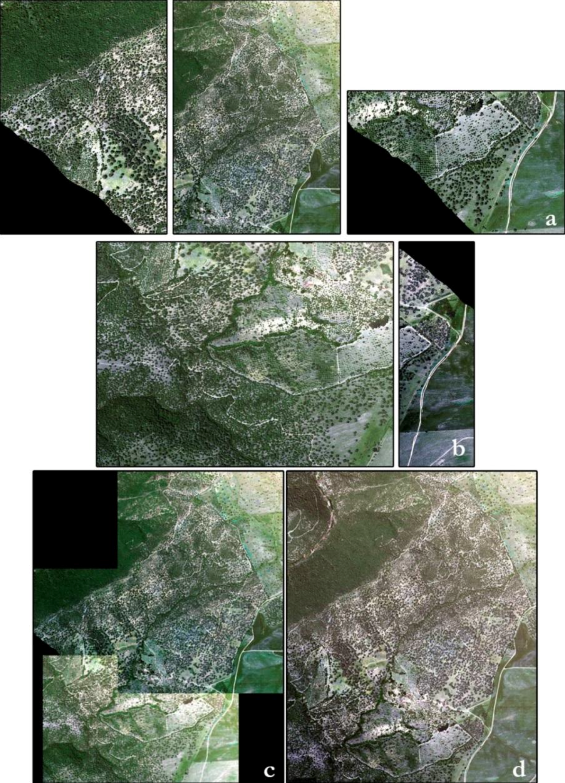
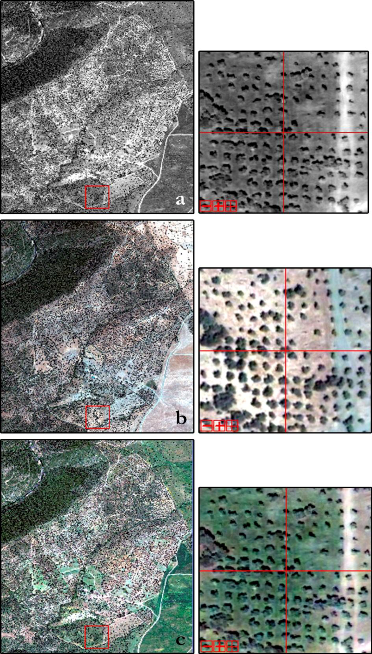
Figure 3 illustrates the QuickBird images from July 2008 and May 2009, fused (60 cm of spatial resolution) and non-fused (240 cm of spatial resolution), and the flight image from May 2009 with resolution of 240 cm after a process of degradation (high to low spatial resolution). At first view, there are no significant differences, except in relation to the color of the images. However, we must be aware that the images were obtained in different seasons and in different years.
Figure 3.
Comparison between images with different spatial resolution: (a) QuickBird 2008 Fused (60 cm); (b) QuickBird 2008 Non-fused (240 cm); (c) QuickBird 2009 Fused (60 cm); (d) QuickBird 2009 Non-fused (240 cm); and (e) Flight 2009 (240 cm).
Figure 3.
Comparison between images with different spatial resolution: (a) QuickBird 2008 Fused (60 cm); (b) QuickBird 2008 Non-fused (240 cm); (c) QuickBird 2009 Fused (60 cm); (d) QuickBird 2009 Non-fused (240 cm); and (e) Flight 2009 (240 cm).
3.2. Assessment of the Mosaic Creation Process
If we analyze the results for images degraded separately, we note that there are differences according to the method of classification and the image used (
Table 3). If we focus on the classifier method, for pass 1 OA applying the ML method varied from 70.10% at 200 cm to 63.19% at 60 cm; for the SVM method, OA was 67.87% at 200 cm, and 63.88% at 60 cm. For the mosaic image, the values ranged from 70.07% at 180 cm to 66.56% at 240 cm for the ML method, while for the SVM method the values were 69.68% at 180 cm and 67.73% at 60 cm. In the case of pass 2, the results were 66.28% at 180 cm and 63.45% at 120 cm for ML, and for SVM they were 66.53% at 60 cm and 63.62% at 240 cm. Overall, there are differences in the accuracy gain between the methods for each image. They are more pronounced in the case of pass 1 and mosaic. However, if we compare between images (
Table 3), there is a general trend to gain accuracy at intermediate spatial resolution, being higher in the case of the mosaic. The method which provided greater accuracy was ML in the case of pass 1 and mosaic, and SVM for pass 2. However, if we analyze the higher accuracy for all images, these results indicate that there is no loss of spectral information in the process of creating mosaics, following the methodology described above.
Table 3.
Analysis of the resolution between images and classifiers based on overall accuracy.
Table 3.
Analysis of the resolution between images and classifiers based on overall accuracy.
| | Pass 1 | Pass 2 | Mosaic |
|---|
| ML | SVM | ML | SVM | ML | SVM |
|---|
| 60 | 63.19 | 63.88 | 64.94 | 66.53 | 67.42 | 67.73 |
| 120 | 64.80 | 64.07 | 63.45 | 64.73 | 69.03 | 67.87 |
| 180 | 67.42 | 66.67 | 66.28 | 65.67 | 70.07 | 69.68 |
| 200 | 70.17 | 67.87 | 64.17 | 65.58 | 70.56 | 68.93 |
| 220 | 68.68 | 66.98 | 65.04 | 64.51 | 66.69 | 68.06 |
| 240 | 67.56 | 64.45 | 65.60 | 63.62 | 66.56 | 69.25 |
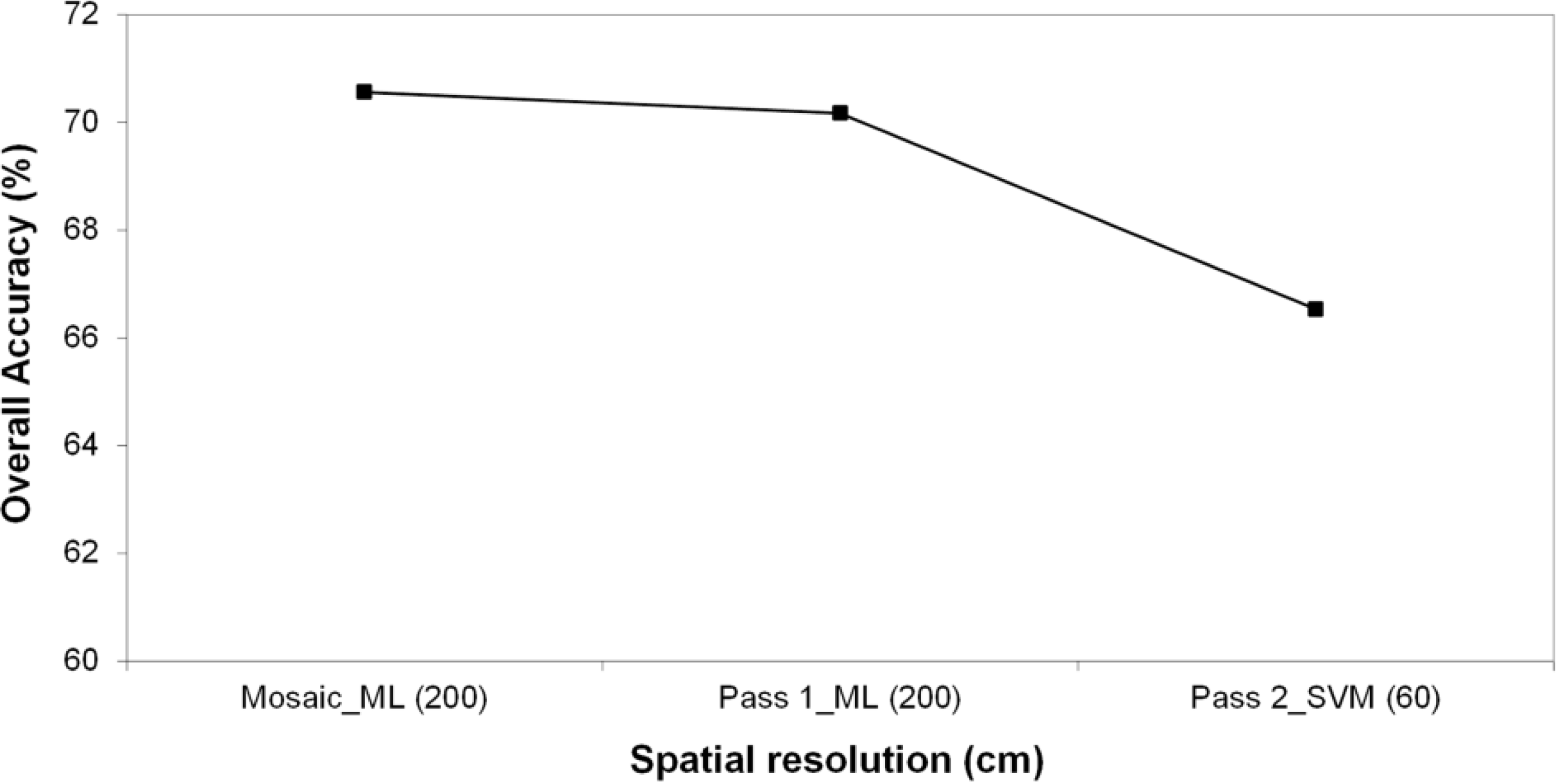
In addition, for the flight image obtained as a mosaic from two separate passes, the maximum value for OA was 70.56% at 200 cm spatial resolution applying the ML method (
Figure 4).
Figure 4.
Comparison between images based on the highest indices.
Figure 4.
Comparison between images based on the highest indices.
3.3. Accuracy Assessment and a Comparison of Overall Classification Accuracy
We used the same degradation methodology as in the previous section for the QuickBird images from July 2008 and May 2009, in order to observe which date gave better results in terms of spatial and spectral resolution. For this purpose, we compared the OV accuracy values for the fused and non-fused images at different spatial resolutions, applying both ML and SVM classification methods, to assess the effect of changing spatial resolution on the performance of the classifiers.
3.3.1. QuickBird Image from 2008
After the fusion and degradation processes of the image from July 2008, the images were classified.
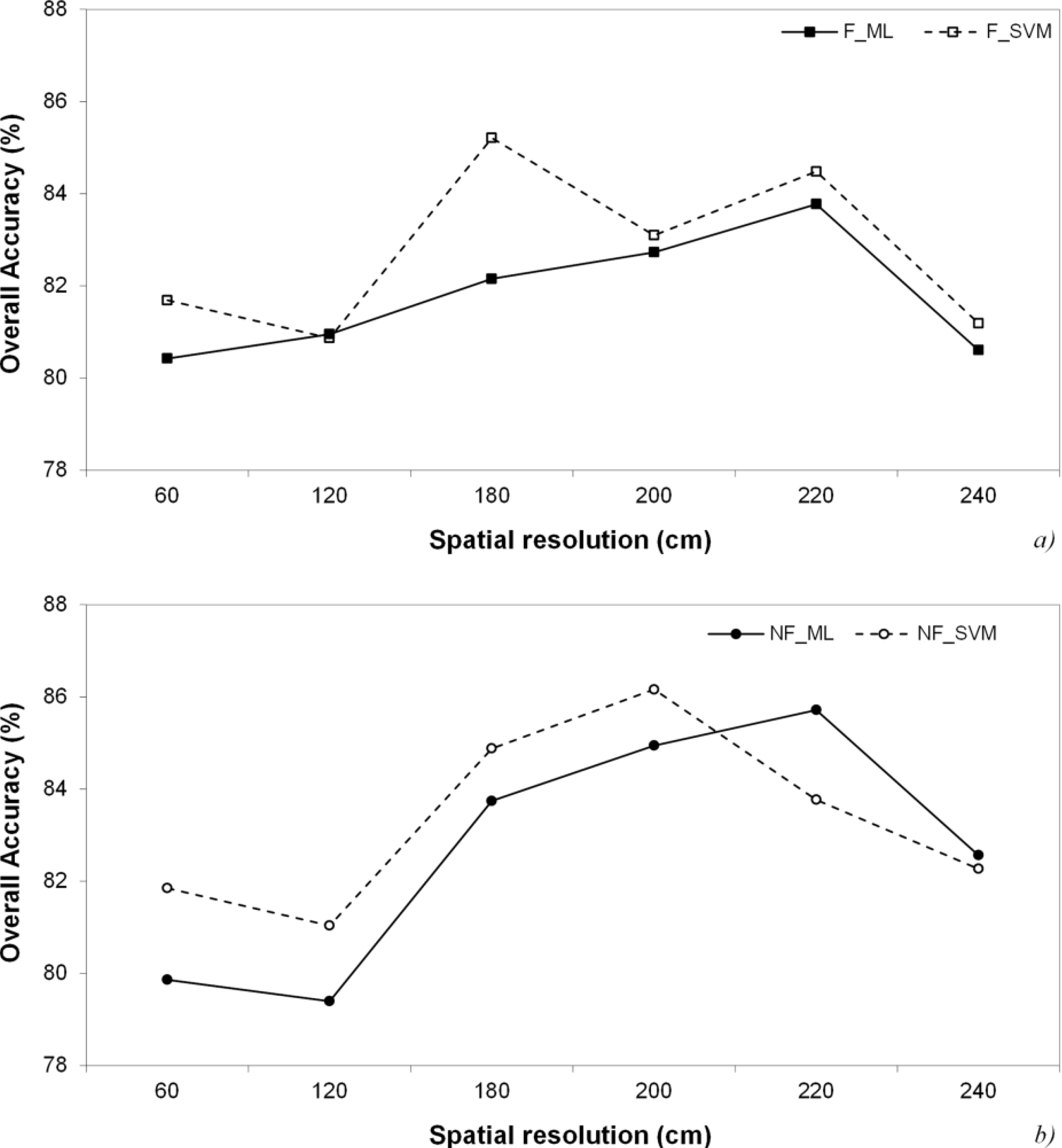
Figure 5 shows the OA values for fused (F) and non-fused (NF) images, left and right respectively, for each classification method.
Figure 5.
Overall accuracy analysis for the QuickBird 2008 image applying ML and SVM classifires: (a) fused image (F); (b) non-fused image (NF).
Figure 5.
Overall accuracy analysis for the QuickBird 2008 image applying ML and SVM classifires: (a) fused image (F); (b) non-fused image (NF).
For the fused image, the OA values ranged between 80.42% at 60 cm of spatial resolution and 83.77% at 220 cm of spatial resolution for the ML classifier, and 80.87% at 120 cm of spatial resolution, and 85.21% at 180 cm of spatial resolution for the SVM classifier. For the non-fused image, the values ranged between 79.39% at 120 cm of spatial resolution, and 85.71% at 220 cm of spatial resolution for the ML classifier, while for the SVM classifier, the values were 81.04% at 120 cm of spatial resolution and 86.16% at 200 cm of spatial resolution.
Therefore, the OA index of the classification for the QuickBird fused image from 2008 took its maximum value (85.21%) at 180 cm of spatial resolution, and for the QuickBird non-fused image from 2008, the maximum OA index (86.16%) was at 200 cm of spatial resolution, in both cases applying the SVM method.
3.3.2. QuickBird Image from 2009
For the QuickBird image from May 2009, we worked in the same way as for the 2008 image. However, the data derived from the classification is considerably different (
Figure 6). For the fused image the OA values ranged between 60.16% at 60 cm of spatial resolution and 64.24% at 200 cm of spatial resolution for the ML classifier, and 52.04% at 240 cm of spatial resolution, and 73.65% at 200 cm of spatial resolution for the SVM classifier. For the non-fused image, the values ranged between 57.12% at 240 cm of spatial resolution, and 65.94% at 200 cm of spatial resolution for the ML classifier, while for the SVM classifier the values were 64.63% at 240 cm of spatial resolution and 71.44% at 180 cm of spatial resolution.
Figure 6.
Overall accuracy analysis for the QuickBird 2009 image applying ML and SVM classifiers: (a) fused image (F); (b) non-fused image (NF).
Figure 6.
Overall accuracy analysis for the QuickBird 2009 image applying ML and SVM classifiers: (a) fused image (F); (b) non-fused image (NF).
Therefore, the OA index of the classification for the QuickBird fused image from 2009 took its maximum value (73.65%) at 200 cm of spatial resolution, and for the non-fused image, the maximum OA index (71.44%) was at 180 cm of spatial resolution, in both cases applying the SVM method.
Table 4 presents a comparison of the highest values of OA, for the QuickBird and aerial flight images at different resolution.
Table 4.
Highest values of overall accuracy for the QuickBird and aerial flight images. Values with symbol a and b were classified with the ML and SVM methods, respectively.
Table 4.
Highest values of overall accuracy for the QuickBird and aerial flight images. Values with symbol a and b were classified with the ML and SVM methods, respectively.
| Spatial Resolution, cm | QB 2008 | QB 2009 | Flight 2009 |
|---|
| F | NF | F | NF |
|---|
| 60 | 81.69 b | 81.85 b | 69.2 b | 70.55 b | 67.73 b |
| 120 | 80.95 a | 81.04 b | 71.89 b | 70.83 b | 69.03 a |
| 180 | 85.21 b | 84.88 b | 72.51 b | 71.44 b | 70.07 a |
| 200 | 83.1 b | 86.16 b | 73.65 b | 70.81 b | 70.56 a |
| 220 | 84.48 b | 85.71 a | 72.57 b | 68.54 b | 68.06 b |
| 240 | 81,19 b | 82.56 a | 63.25 a | 64.63 b | 69.25 b |
Therefore, after applying a supervised classification by the Support Vector Machine method, based on selected regions of interest (ROIs) (Pyrus, Olea, Quercus, wet grass, dry grass, mixed woodland, riparian forest, soil, saturated soil, ponds and shade), the highest values in the classification were obtained for the QuickBird July 2008 image, non-fused and at 200 cm of spatial resolution.
To assess the performance of the two methods of classification (ML and SVM) through the statistical significance of the differences in overall accuracy, we used the July 2008 Quickbird image because it provided the highest overall accuracy values for all studied spatial resolutions (
Table 4). The results of the McNemar Chi-squared test after comparing pairs of overall accuracy values (
Table 5) were statistically significant in the following cases: at 60 cm (NF), 120 cm (NF) and 180 cm (F) SVM outperforms ML (
p < 0.001). However, ML performed better than SVM at 220 cm (NF) of resolution (
p < 0.05). There are no significant differences between the classifiers at 200 cm (NF) and 240 cm (NF) of resolution. Therefore, for high-spatial resolution, the SVM classifier performs better than ML, with significant increases in overall accuracy. However, from 2 meters of spatial resolution, the highest overall accuracy values change for the ML classifier, but the statistical significance is lower or even disappears.
Table 5.
The McNemar Chi-squared test for comparing the overall accuracy (%) of the classifications by ML and SVM methods in the July 2008 Quickbird image with different spatial resolutions. Significant differences are indicated as ns (not significant); * (p < 0.05); *** (p < 0.001).
Table 5.
The McNemar Chi-squared test for comparing the overall accuracy (%) of the classifications by ML and SVM methods in the July 2008 Quickbird image with different spatial resolutions. Significant differences are indicated as ns (not significant); * (p < 0.05); *** (p < 0.001).
| Image | Resolution | ML | SVM | Chi-Square |
|---|
| QB08 NF | 60 | 79.86 | 81.85 | 28.1 *** |
| QB08 NF | 120 | 79.39 | 81.04 | 10.4 *** |
| QB08 F | 180 | 82.15 | 85.21 | 30.1 *** |
| QB08 NF | 200 | 84.94 | 86.16 | 1.2 ns |
| QB08 NF | 220 | 85.71 | 83.77 | 4.1 * |
| QB08 NF | 240 | 82.56 | 82.27 | 0.2 ns |
3.4. Comparison between Images According to the Pyrus Class
As is already known, the producer’s accuracy (PA) is based on the number of pixels that are classified as
Pyrus and actually are
Pyrus, from the total real pixels of the
Pyrus class. The user’s accuracy (UA) corresponds to the successes, and is based on the number of pixels classified as
Pyrus that are in fact
Pyrus, from the total number of pixels classified as
Pyrus. In this sense,
Table 6 shows the PA and UA values for the class
Pyrus, for each type of image analyzed.
Table 6.
Comparison between images based in the producer and user (P/U) index values for the Pyrus class. Values with symbol a and b were classified with the ML and SVM methods, respectively. For the Flight 2009 image, left and right, respectively.
Table 6.
Comparison between images based in the producer and user (P/U) index values for the Pyrus class. Values with symbol a and b were classified with the ML and SVM methods, respectively. For the Flight 2009 image, left and right, respectively.
Spatial
Resolution | QB 2008 | QB 2009 | Flight 2009 |
|---|
| F a | NF a | F b | NF b | F a | NF a | F b | NF b |
|---|
| 60 | 39.9/37.2 | 23.6/40.2 | 32.0/50.6 | 16.4/28 | 14.3/6.8 | 28.8/14.8 | 8.4/36 | 21/11.1 | 35.7/28.9 | 22.5/38.3 |
| 120 | 37.5/43.6 | 19.2/28.9 | 27.3/49.3 | 10.4/17.3 | 25.4/9.9 | 29.1/12.5 | 5.6/6.6 | 5/6.2 | 30.8/23.9 | 20.3/42.8 |
| 180 | 40.7/36.6 | 29.8/36.9 | 22.2/44.4 | 14/32 | 40/16.5 | 34.2/14.6 | 18.1/15 | 10.1/13.7 | 38.2/20.8 | 8.8/16.6 |
| 200 | 43.5/39.2 | 38.8/46.3 | 17.4/38.1 | 16.3/33.3 | 31.1/10.5 | 12.1/13.8 | 2.2/10.3 | 9.3/11 | 27.1/19.7 | 7.5/14.3 |
| 220 | 45.7/42.1 | 40/45.1 | 20/36.8 | 8.5/21.4 | 29.2/13.3 | 7.4/5.8 | 10/15.6 | 8.8/10.3 | 44/21.8 | 4/15.8 |
| 240 | 43.5/55.5 | 47.8/44 | 15.2/33.3 | 30.4/40 | 51.5/20.7 | 15.8/7.9 | 3.3/12 | 4/9.7 | 47/21.9 | 8.8/14.8 |
For the fused image from July 2008, the maximum classification value (OA = 85.21%) at 180 cm resolution, presents values of 40.74% for PA and 36.67% for UA, applying the SVM method. However, for a resolution of 240 cm and applying the ML classifier, the OA classification value is lower (80.60%), but it presents the highest values of 43.48% for the producer and 55.56% for the user. Moreover, the results are different for the non-fused image from July 2008. The highest OA value (86.16%) is given at 200 cm resolution, applying the SVM method, with 16.33% for PA and 33.33% for UA. However, as in the case of the fused image, the OA classification data is a few points lower (84.94%) at 200 cm of resolution, but the UA values are reinforced (producer: 38.78%; user: 46.34%) when we apply the ML method.
For the image from May 2009, we analyzed the PA and UA values in the same way. The maximum classification values for the fused image (OA = 73.65%) when we apply the SVM method at 200 cm resolution, are 2.22% for PA and 10.33% for UA. For resolution of 60 cm, the classification values (OA = 69.2%) are higher at 8.4% for PA and 36% for UA, also when the SVM method is applied. However, the results are different for the non-fused image from 2009. When we apply the SVM classifier, the highest OA value (71.44%) is at 180 cm, with 10.12% PA and 13.79% UA. However, when we apply the ML method, the OA classification data is a few points lower (65.02%) at 60 cm resolution, but the accuracy values are reinforced (producer: 28.83%; user: 14.88%).
Finally, for the flight 2009 images, the highest OA value (70.56) is at 200 cm of resolution when we apply the ML method, with 27.1% PA and 19.7% UA. However, the maximum classification values are at 120 cm of resolution (OA = 67.87) applying the SVM classifier, with 20.3% PA and 42.8% UA.
We analyze below the results of the error matrices with the highest classification values for the QuickBird fused image from July 2008 at 240 cm of resolution and classified by the ML method (
Table 7), for the QuickBird fused image from May 2009 at 60 cm and classified by the SVM method (
Table 8), and from the Flight 2009 image at 120 cm and classified by the SVM method (
Table 9).
For the image from July 2008, the PA for the individual categories ranged between 25.81% for the Olea class and 95.28% for the dry grass class, while the UA was between 10.13% for the Olea class and 100% for the soil and saturated soil classes. The Pyrus class provided UA of 55.56% and PA of 43.48%. The classification recognizes some of the pixels of the Pyrus class, like other vegetation formations, mainly Olea, even with shadows. The results change considerably when we analyze the image from May 2009. The PA ranged from 8.38% for the Pyrus class to 99.72% for the soil class, whereas the UA ranged between 22.89% for the saturated soil class and 99.76% for the wet grass class. The Pyrus class provided UA of 35.9% and PA of 8.38%. In this case, the classification mistook most of the pixels of the Pyrus class for the Quercus, mixed woodland and dry grass classes. In the case of the Flight 2009 image, PA ranged from 19.52% for the Quercus class to 99.72% for the Soil class, whereas UA ranged between 30.63% for the Olea class and 99.67% for the saturated soil class. The Pyrus class provided UA of 42.86% and PA of 20.37%. In this case, the classification mistook most of the pixels of the Pyrus class for the Olea class.
Table 7.
Error matrix of the QuickBird fused image from July 2008 at 240 cm of resolution and classified by the ML method.
Table 7.
Error matrix of the QuickBird fused image from July 2008 at 240 cm of resolution and classified by the ML method.
| Classified Category | Actual Category | Total | User’s Accuracy (%) |
|---|
| Pyrus | Olea | Quercus | Wet grass | Dry Grass | Mixed Woodland | Riparian Forest | Soil | Saturated Soil | Ponds | Shade |
|---|
| Pyrus | 20 | 6 | 1 | 2 | 2 | 2 | 0 | 0 | 0 | 0 | 3 | 36 | 55.56 |
| Olea | 9 | 8 | 7 | 2 | 0 | 26 | 0 | 15 | 5 | 3 | 4 | 79 | 10.13 |
| Quercus | 7 | 9 | 90 | 0 | 0 | 4 | 0 | 0 | 0 | 0 | 1 | 111 | 81.08 |
| Wet Grass | 0 | 2 | 0 | 89 | 0 | 0 | 3 | 0 | 0 | 0 | 0 | 94 | 94.68 |
| Dry Grass | 0 | 0 | 0 | 0 | 101 | 0 | 0 | 1 | 4 | 0 | 4 | 110 | 91.82 |
| Mixed Woodland | 6 | 4 | 14 | 0 | 0 | 133 | 15 | 0 | 0 | 1 | 1 | 174 | 76.44 |
| Riparian Forest | 0 | 1 | 2 | 7 | 0 | 0 | 85 | 0 | 0 | 0 | 0 | 95 | 89.47 |
| Soil | 0 | 0 | 0 | 0 | 0 | 0 | 0 | 74 | 0 | 0 | 0 | 74 | 100 |
| Saturated Soil | 0 | 0 | 0 | 0 | 0 | 0 | 0 | 0 | 87 | 0 | 0 | 87 | 100 |
| Ponds | 0 | 0 | 2 | 0 | 0 | 1 | 0 | 0 | 0 | 50 | 3 | 56 | 89.29 |
| Shade | 4 | 1 | 5 | 0 | 3 | 0 | 0 | 0 | 1 | 5 | 86 | 105 | 81.90 |
| Total | 46 | 31 | 121 | 100 | 106 | 166 | 103 | 90 | 97 | 59 | 102 | |
| Producer’s Accuracy (%) | 43.48 | 25.81 | 74.38 | 89 | 95.28 | 80.12 | 82.52 | 82.22 | 89.69 | 84.75 | 84.31 |
Table 8.
Error matrix of the QuickBird fused image from May 2009 at 60 cm and classified by the SVM method.
Table 8.
Error matrix of the QuickBird fused image from May 2009 at 60 cm and classified by the SVM method.
| Classified Category | Actual Category | Total | User’s Accuracy (%) |
|---|
| Pyrus | Olea | Quercus | Wet Grass | Dry Grass | Mixed Woodland | Riparian Forest | Soil | Saturated Soil | Ponds | Shade |
|---|
| Pyrus | 42 | 5 | 28 | 0 | 9 | 26 | 2 | 0 | 0 | 0 | 5 | 117 | 35.9 |
| Olea | 28 | 83 | 86 | 0 | 1 | 0 | 0 | 0 | 0 | 0 | 0 | 198 | 41.92 |
| Quercus | 103 | 68 | 949 | 0 | 51 | 346 | 32 | 0 | 0 | 2 | 49 | 1600 | 59.31 |
| Wet Grass | 0 | 3 | 0 | 1269 | 0 | 0 | 0 | 0 | 0 | 0 | 0 | 1272 | 99.76 |
| Dry Grass | 38 | 54 | 137 | 0 | 1369 | 39 | 18 | 0 | 0 | 0 | 2 | 1657 | 82.62 |
| Mixed Woodland | 239 | 112 | 460 | 9 | 0 | 2110 | 504 | 0 | 0 | 2 | 94 | 3530 | 59.77 |
| Riparian Forest | 27 | 129 | 152 | 225 | 0 | 0 | 955 | 0 | 0 | 0 | 0 | 1488 | 64.18 |
| Soil | 0 | 0 | 3 | 0 | 11 | 0 | 0 | 1447 | 7 | 0 | 0 | 1468 | 98.57 |
| Saturated Soil | 0 | 0 | 14 | 0 | 403 | 0 | 0 | 4 | 125 | 0 | 0 | 546 | 22.89 |
| Ponds | 2 | 0 | 1 | 0 | 0 | 36 | 4 | 0 | 0 | 655 | 354 | 1052 | 62.26 |
| Shade | 22 | 3 | 56 | 0 | 0 | 118 | 2 | 0 | 0 | 358 | 1072 | 1631 | 65.73 |
| Total | 501 | 457 | 1886 | 1503 | 1844 | 2675 | 1517 | 1451 | 132 | 1017 | 1576 | |
| Producer’s Accuracy (%) | 8.38 | 18.16 | 50.32 | 84.43 | 74.24 | 78.88 | 62.95 | 99.72 | 94.70 | 64.41 | 68.02 |
Table 9.
Error matrix of the Flight 2009 image at 120 cm and classified by the SVM method.
Table 9.
Error matrix of the Flight 2009 image at 120 cm and classified by the SVM method.
| ClassifiedCategory | Actual Category | Total | User’s Accuracy (%) |
|---|
| Pyrus | Olea | Quercus | Wet Grass | Dry Grass | Mixed Woodland | Riparian Forest | Soil | Saturated Soil | Ponds | Shade |
|---|
| Pyrus | 33 | 43 | 0 | 0 | 0 | 0 | 0 | 0 | 0 | 0 | 1 | 77 | 42.86 |
| Olea | 46 | 34 | 0 | 0 | 0 | 0 | 29 | 0 | 0 | 0 | 2 | 111 | 30.63 |
| Quercus | 7 | 9 | 90 | 0 | 31 | 46 | 19 | 0 | 0 | 0 | 29 | 231 | 38.96 |
| Wet Grass | 3 | 0 | 3 | 321 | 9 | 104 | 69 | 0 | 0 | 0 | 0 | 509 | 63.06 |
| Dry Grass | 1 | 0 | 10 | 18 | 335 | 6 | 0 | 0 | 1 | 0 | 10 | 381 | 87.93 |
| Mixed Woodland | 25 | 20 | 258 | 63 | 2 | 379 | 39 | 0 | 0 | 0 | 15 | 801 | 47.32 |
| Riparian Forest | 42 | 25 | 91 | 6 | 22 | 128 | 243 | 0 | 0 | 0 | 2 | 559 | 43.47 |
| Soil | 0 | 0 | 0 | 0 | 0 | 0 | 0 | 362 | 2 | 0 | 0 | 364 | 99.45 |
| Saturated Soil | 0 | 0 | 0 | 0 | 0 | 0 | 0 | 1 | 300 | 0 | 0 | 301 | 99.67 |
| Ponds | 0 | 0 | 0 | 0 | 0 | 0 | 0 | 0 | 0 | 248 | 10 | 258 | 96.12 |
| Shade | 5 | 0 | 9 | 0 | 0 | 10 | 2 | 0 | 0 | 2 | 349 | 377 | 92.57 |
| Total | 162 | 131 | 461 | 408 | 399 | 673 | 401 | 363 | 303 | 250 | 418 | |
| Producer’s Accuracy (%) | 20.37 | 25.95 | 19.52 | 78.68 | 83.96 | 56.32 | 60.60 | 99.72 | 99.01 | 99.20 | 83.49 |
4. Discussion
The degradation process at different spatial resolutions which was carried out over the images allowed smoothed images to be obtained which are much more useful for distinguishing shapes, features and sizes, especially for the small-size of the crown of
P. bourgaeana. In addition, the analysis of the aerial flight images showed that the construction of mosaics from “parts” of an image, following the methodology described in this paper, facilitates the treatment of these parts without losing spectral information [
61,
62]. Thus, for the flight image from 2009, obtained as a mosaic, the maximum overall accuracy value (70.56%) was for the image with spatial resolution of 200 cm, applying the Maximum Likelihood method and having statistically significant differences (McNemar test Chi-square = 18.1,
p < 0.05) from the Support Vector Machine method.
We applied the same methodology for the mosaic image as for the QuickBird images from July 2008 and May 2009, in order to observe which date gave better results in terms of spatial, spectral and temporal resolution, based on the classification results. In this case, the comparison was made between fused images by the IHS method and non-fused images, for the same date and between different dates. Visual analysis of the QuickBird images with different levels of degradation, and after applying two supervised classification methods (Maximum Likelihood and Support Vector Machine), showed that there were no significant differences. However, slight differences did appear in the color of the images, because they had been obtained in different months.
After applying two different classification methods over Quickbird fused images and non-fused images, with different spatial resolution and from different seasons, the highest overall accuracy values were obtained for the July 2008 image. For the fused image, the overall accuracy value was of 85.21% at 180 cm of spatial resolution, and for the non-fused image the overall accuracy was of 86.16% at 200 cm of spatial resolution. However, the overall accuracy for the QuickBird fused image from 2009 took its maximum value of 73.65% at 200 cm of spatial resolution, and for the non-fused image the maximum value was 71.44% at 180 cm of spatial resolution. For all cases, the classification method was the Support Vector Machine algorithm.
These results are in consonance with what has been reported by other authors [
63]—the superior performance of the SVM method compared with the ML method. However, when we compared the highest overall accuracy values corresponding with the July 2008 QuickBird image, the differences between the two algorithms were in some cases not significant. The McNemar Chi-squared test demonstrated that there were differences depending on the spatial resolution that was used. A comparison of the overall accuracy values revealed that the use of any classifier at intermediate spatial resolution (180–200 cm) was superior to the corresponding classifier with higher and lower resolutions, since the overall accuracy increases when the pixel size is larger. However, the statistical significance varied from higher spatial resolution to lower spatial resolution, and was more pronounced for higher spatial resolution. A possible explanation for the lower accuracies of the high spectral resolution images is that the smaller pixel size introduced higher spectral variance within a class, and this resulted in lower spectral separability among the classes. However, at low spatial resolution, the spectral signatures of the different classes became over-generalized, and the spectral separability within each pixel was reduced. This approach could also explain the slight difference between the fused image and the non-fused image. Therefore the highest overall accuracy values were found at 1.8–2 m pixel size, regardless of the classification method that was used.
Furthermore, the accuracy at class level may differ between algorithms, and may thus influence the choice of one classifier or the other, depending on purposes of the user. The analysis of the user’s accuracy data and the producer’s accuracy data for the Pyrus class showed that the differences are highly dependent on the date of acquisition, on degradation, and on the type of image (fused and non-fused). If there are differences in any of these characteristics of the image, the overall rates can be reinforced at the expense of the partial indices, and vice versa. Although the results in terms of overall classification were lower than for the non-fused image, and there were no significant differences in terms of overall accuracy when we compared the classification methods (McNemar Chi-squared test = 0.25, ns), the QuickBird image from July 2008, fused by the IHS method, degraded at 240 cm spatial resolution and classified by the Maximum Likelihood method, provided accuracy values higher than 55% when classifying wild pears in the study area (producer’s accuracy = 43.48% and user’s accuracy = 55.56%). The Maximum Likelihood algorithm identified the Pyrus class with greater accuracy than SVM, even with differences among classifiers of 28.26% for PA and 22.23% for UA.
A hypothesis that can explain why the overall classification is better for the image of July is that
P. bourgaeana can still maintain a considerably percentage of green leaves on its branches during the summer, as evidenced by its phenological cycle, in which the vegetative development extends from March to early August. There may be confusion with other vegetation because, at this time of the year, the spectral response of vegetation and mainly deciduous trees, such as wild pear, is strongly influenced by the process of leaves senescence and shedding, mainly related to the summer drought. It would therefore be advisable to capture the selected scene at a date between the end of spring and early summer. However, the lowest results extracted from the QuickBird image from May 2009 revealed that the greatest confusion is among vegetation classes. This may be mainly due to the overlap between the crowns of the trees, pastures and scrub, because in springtime most plant species foliate and flower at the same time, and this may lead to an overlap between spectral signatures. This could be confirmed by an analysis of the spectral differences between the wild pear and the surrounding vegetation, based on their spectral signature and by analyzing hyperspectral information, in order to minimize the effect of spectral overlap [
64,
65].
The small crown size of this species and its low abundance and scattered distribution across the Mediterranean evergreen forest and open woodland (dehesa), make the individual trees difficult to locate, limiting the search and selection of pixels required to carry out such studies. We must take into account that factors such as the density or the morphology of the leaves of the crown, and the shadows that they project, could influence the classification results [
66]. Even with a manual delineation of the crowns, the yield of the classification may be low [
67]. Clearly, it is a difficult task to classify, from multispectral images (less than 50%), individual trees of limited size, immersed in a matrix of mixed vegetation, especially when their crowns overlap to some extent [
68,
69]. However, although this process, which was based on the interpretation of single pixels, has improved the visual and spectral quality of the multispectral images, we are considering the use of hyperspectral data in the future to improve the classification results. In addition, other techniques could be also tested in future work, such as object classification applied to the original images based on groups of pixels [
70].
5. Conclusions
The degradation process at different spatial resolutions that was carried out over the images enabled us to discriminate shapes, features and sizes, especially for the small-sized crown of P. bourgaeana, without losing spectral information.
Both the Maximum Likelihood and Support Vector Machines algorithms performed moderately well for discriminating individual P. bourgaeana trees from color-infrared images of QuickBird and aerial orthophotos obtained from the ADS40-SH52 airborne sensor, achieving overall accuracies higher than or equal to 86%. In general, Support Vector Machines gave better accuracies than the Maximum Likelihood algorithm for all fused and non-fused images. In fact, the highest overall accuracy value was provided by Support Vector Machines for the July 2008 Quickbird non-fused image at 200 cm of spatial resolution, reaching the highest values at intermediate-low spatial resolution. In addition, it was better than Maximum Likelihood for images with high spatial resolution, having significant differences in overall accuracy. However, the QuickBird image from July 2008, fused by the IHS method, degraded at 240 cm spatial resolution and classified by the Maximum Likelihood method, provided the highest accuracy values for the Pyrus class (producer’s accuracy = 43.48% and user’s accuracy = 55.56%).
The results provided in this study, although modest, provide a valuable starting point to understand the distribution and the spatial structure of P. bourgaeana, aimed at improving and prioritizing conservation efforts. Furthermore, the approach used in this work might be also applied to other taxa, and might also benefit from future improvements in both the quality of remote sensing imaginary and the methods of analysis.


