Urban-Tree-Attribute Update Using Multisource Single-Tree Inventory

 ,
,  ,
,
Abstract
:1. Introduction
2. Materials
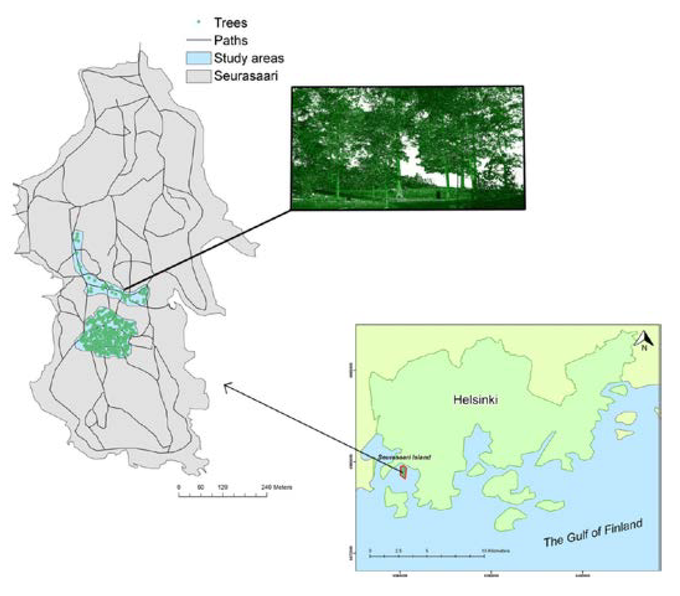
2.1. Study Area

| Species | % |
|---|---|
| Acer platanoides | 2.64 |
| Alnus sp. | 9.13 |
| Betula sp. | 7.30 |
| Picea abies | 25.96 |
| Pinus sylvestris | 19.88 |
| Populus tremula | 9.94 |
| Quercus robur | 6.69 |
| Salix caprea | 0.81 |
| Sorbus aucuparia | 14.60 |
| Tilia cordata | 2.43 |
| Ulmus sp. | 0.61 |
2.2. Field Measurements
2.3. Airborne Laser Scanning
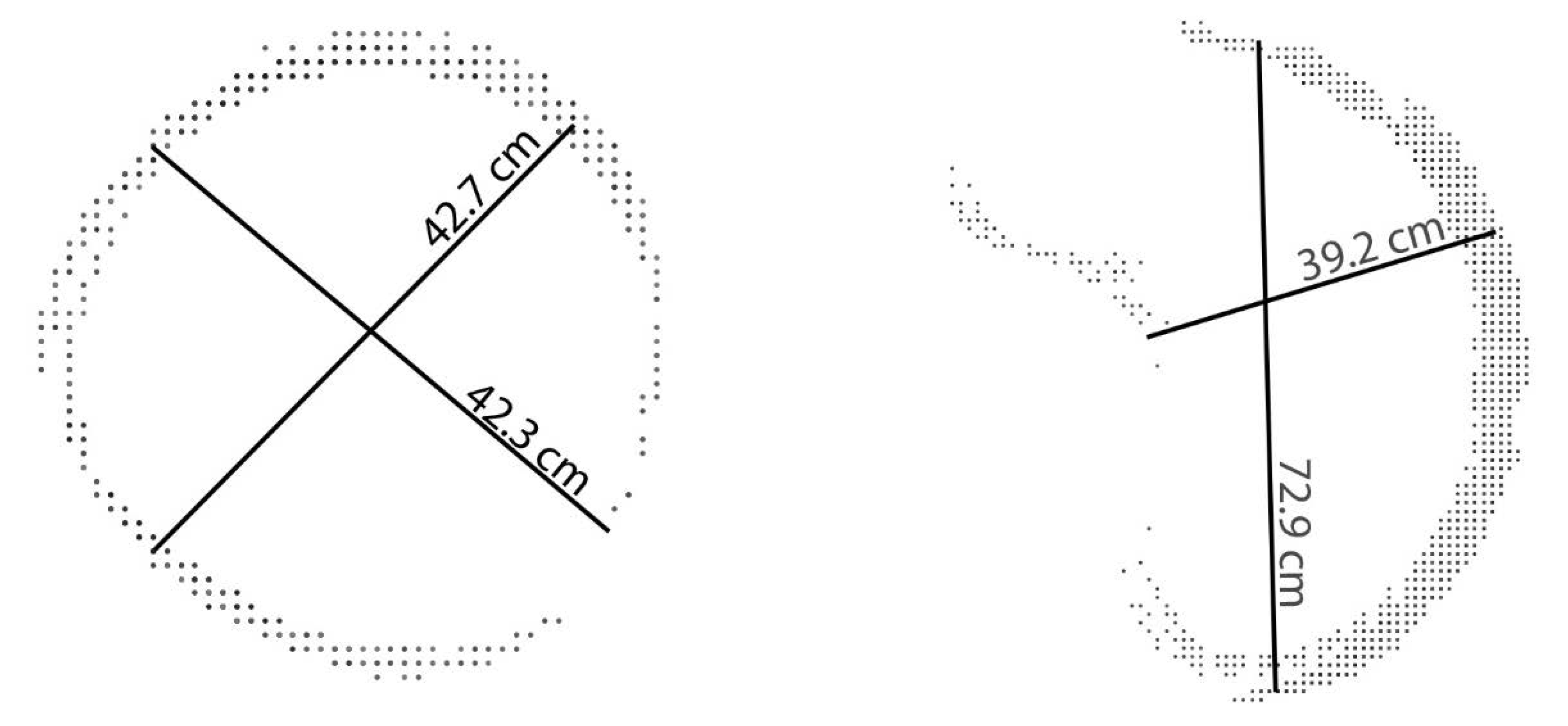
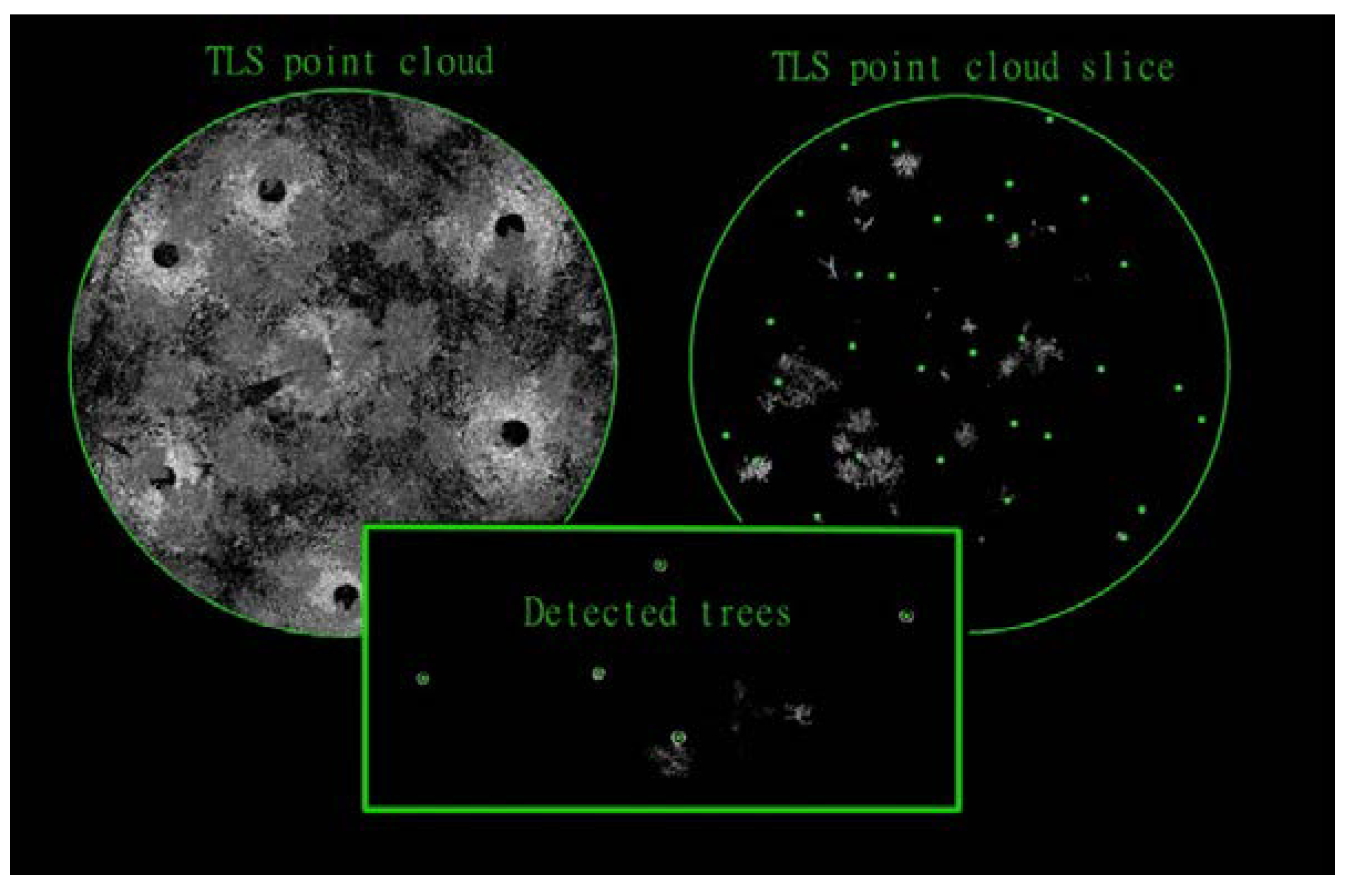
2.4. Terrestrial Laser Scanning
| Leica HDS6100 System | Specifications |
|---|---|
| Field of View | 310° × 360° |
| Range | 79 m |
| Speed Points/s | 508,000 |
| Spot Size | 3 mm + 0.22 mrad |
| Distance Measurement Accuracy at 25 m | ±2 mm |
| Max Resolution | 0.009° Hor × 0.009° Ver |
| Max Points 360° | 40,000 Hor × 40,000 Ver |
| Laser Wavelength | 690 nm |
| Laser Power | 30 mW |
| Weight | 14 kg |
| Operating Temperature | −10 to 45 °C |
3. Multisource Single-Tree Inventory
3.1. TLS-Based Tree Map
3.2. Extraction of Tree Height, Crown Area, and the Prediction Variables from the ALS Data
| Variable | Forest | Park | ||||||||
|---|---|---|---|---|---|---|---|---|---|---|
| Min | Max | Range | Mean | Std | Min | Max | Range | Mean | Std | |
| Hmax | 4.54 | 29.15 | 24.61 | 19.68 | 5.26 | 7.76 | 26.04 | 18.28 | 19.44 | 4.90 |
| Hmean | 3.14 | 22.95 | 19.81 | 12.99 | 4.19 | 4.84 | 23.09 | 18.25 | 12.73 | 4.44 |
| Hstd | 0.64 | 9.11 | 8.47 | 4.30 | 1.50 | 1.43 | 6.82 | 5.38 | 4.47 | 1.33 |
| Vege | 0.25 | 1.00 | 0.75 | 0.71 | 0.15 | 0.35 | 0.94 | 0.58 | 0.65 | 0.13 |
| CV | 0.08 | 0.91 | 0.82 | 0.35 | 0.11 | 0.24 | 0.56 | 0.32 | 0.37 | 0.09 |
| h10 | 1.13 | 20.03 | 18.90 | 6.98 | 3.64 | 2.20 | 19.04 | 16.84 | 6.50 | 3.72 |
| h20 | 1.95 | 21.25 | 19.30 | 9.39 | 4.20 | 3.20 | 24.56 | 21.36 | 8.85 | 5.40 |
| h30 | 2.14 | 23.77 | 21.63 | 11.08 | 4.45 | 3.86 | 24.94 | 21.08 | 10.51 | 5.14 |
| h40 | 2.64 | 24.01 | 21.38 | 12.41 | 4.63 | 4.67 | 25.14 | 20.47 | 12.08 | 5.16 |
| h50 | 2.96 | 24.19 | 21.23 | 13.60 | 4.77 | 5.15 | 25.24 | 20.10 | 13.54 | 5.20 |
| h60 | 3.42 | 24.31 | 20.89 | 14.66 | 4.89 | 5.57 | 25.30 | 19.73 | 14.66 | 5.06 |
| h70 | 3.75 | 24.38 | 20.63 | 15.77 | 4.94 | 5.78 | 25.40 | 19.62 | 15.64 | 4.99 |
| h80 | 4.11 | 24.72 | 20.61 | 16.81 | 5.04 | 6.08 | 25.46 | 19.38 | 16.71 | 4.85 |
| h90 | 4.44 | 26.75 | 22.31 | 17.97 | 5.09 | 6.60 | 25.62 | 19.02 | 17.86 | 4.88 |
| p10 | 0.00 | 0.21 | 0.21 | 0.03 | 0.03 | 0.00 | 0.10 | 0.10 | 0.01 | 0.02 |
| p20 | 0.00 | 0.67 | 0.67 | 0.07 | 0.08 | 0.00 | 0.25 | 0.25 | 0.07 | 0.06 |
| p30 | 0.00 | 0.77 | 0.77 | 0.12 | 0.12 | 0.01 | 0.35 | 0.34 | 0.14 | 0.09 |
| p40 | 0.00 | 0.96 | 0.96 | 0.19 | 0.16 | 0.03 | 0.46 | 0.43 | 0.22 | 0.11 |
| p50 | 0.00 | 0.98 | 0.98 | 0.27 | 0.18 | 0.07 | 0.53 | 0.46 | 0.31 | 0.13 |
| p60 | 0.00 | 0.98 | 0.98 | 0.38 | 0.19 | 0.10 | 0.65 | 0.56 | 0.42 | 0.16 |
| p70 | 0.00 | 0.98 | 0.98 | 0.50 | 0.20 | 0.10 | 0.77 | 0.68 | 0.53 | 0.19 |
| p80 | 0.02 | 0.98 | 0.97 | 0.65 | 0.18 | 0.14 | 0.89 | 0.75 | 0.67 | 0.20 |
| p90 | 0.19 | 0.99 | 0.80 | 0.82 | 0.14 | 0.16 | 0.97 | 0.81 | 0.79 | 0.22 |
3.3. Estimation of the Tree Variables
3.4. Accuracy Assessment at the Tree and Stand Level

4. Results
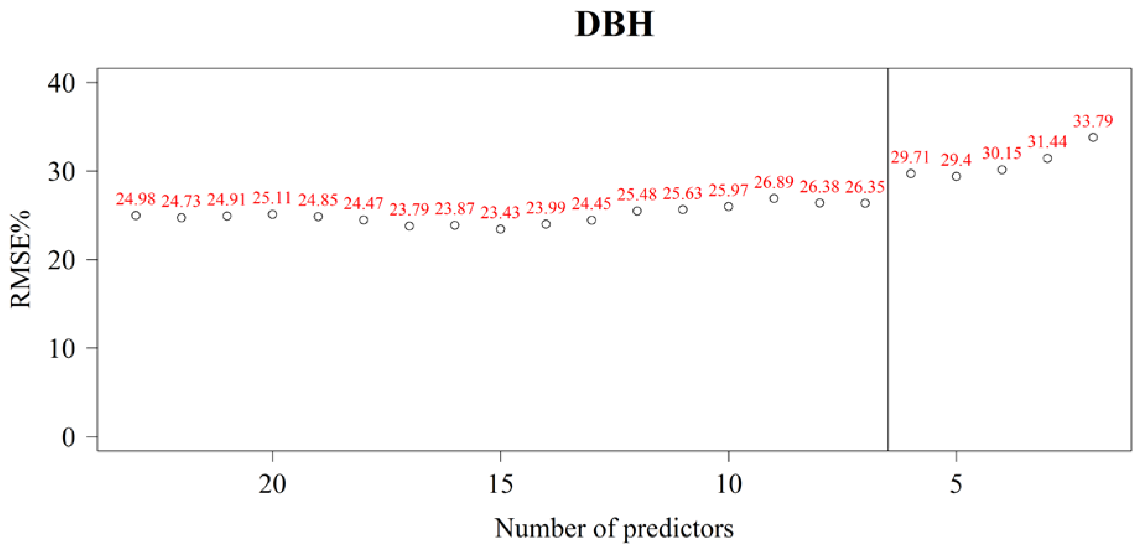
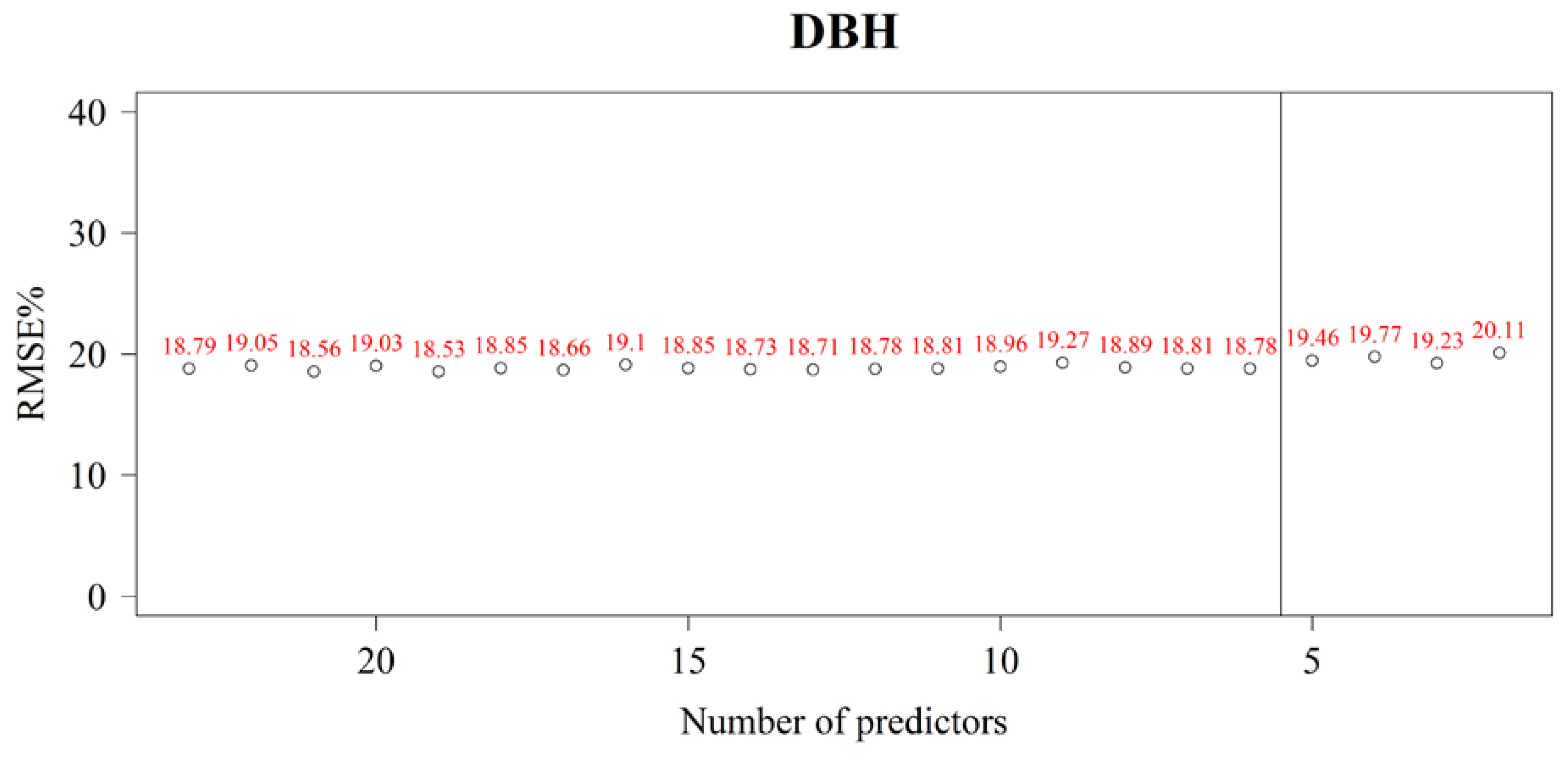
4.1. Selecting Predictor Variables

| Forest | Park |
|---|---|
| h50 | h90 |
| Hmean | p80 |
| h60 | h70 |
| h70 | h60 |
| h40 | p90 |
| h20 | Hmax |
| p10 |

4.2. Prediction Accuracy of Diameter-at-Breast Height

| Number of Neighbors | Forest | Park | ||||||
|---|---|---|---|---|---|---|---|---|
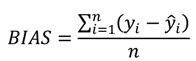
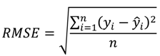
| BIAS, cm | BIAS-% | RMSE, cm | RMSE-% | BIAS, cm | BIAS-% | RMSE, cm | RMSE-% | |
| k = 1 | −0.66 | −2.53 | 7.58 | 29.11 | 0.67 | 1.81 | 3.97 | 10.70 |
| k = 2 | −0.17 | −0.64 | 7.15 | 27.45 | −0.15 | −0.41 | 5.63 | 15.18 |
| k = 3 | −0.22 | −0.85 | 7.06 | 27.08 | −0.39 | −1.05 | 6.63 | 17.90 |
| k = 4 | −0.15 | −0.58 | 6.93 | 26.62 | −1.06 | −2.86 | 6.77 | 18.27 |
| k = 5 | −0.11 | −0.41 | 6.85 | 26.29 | −1.56 | −4.21 | 7.09 | 19.12 |
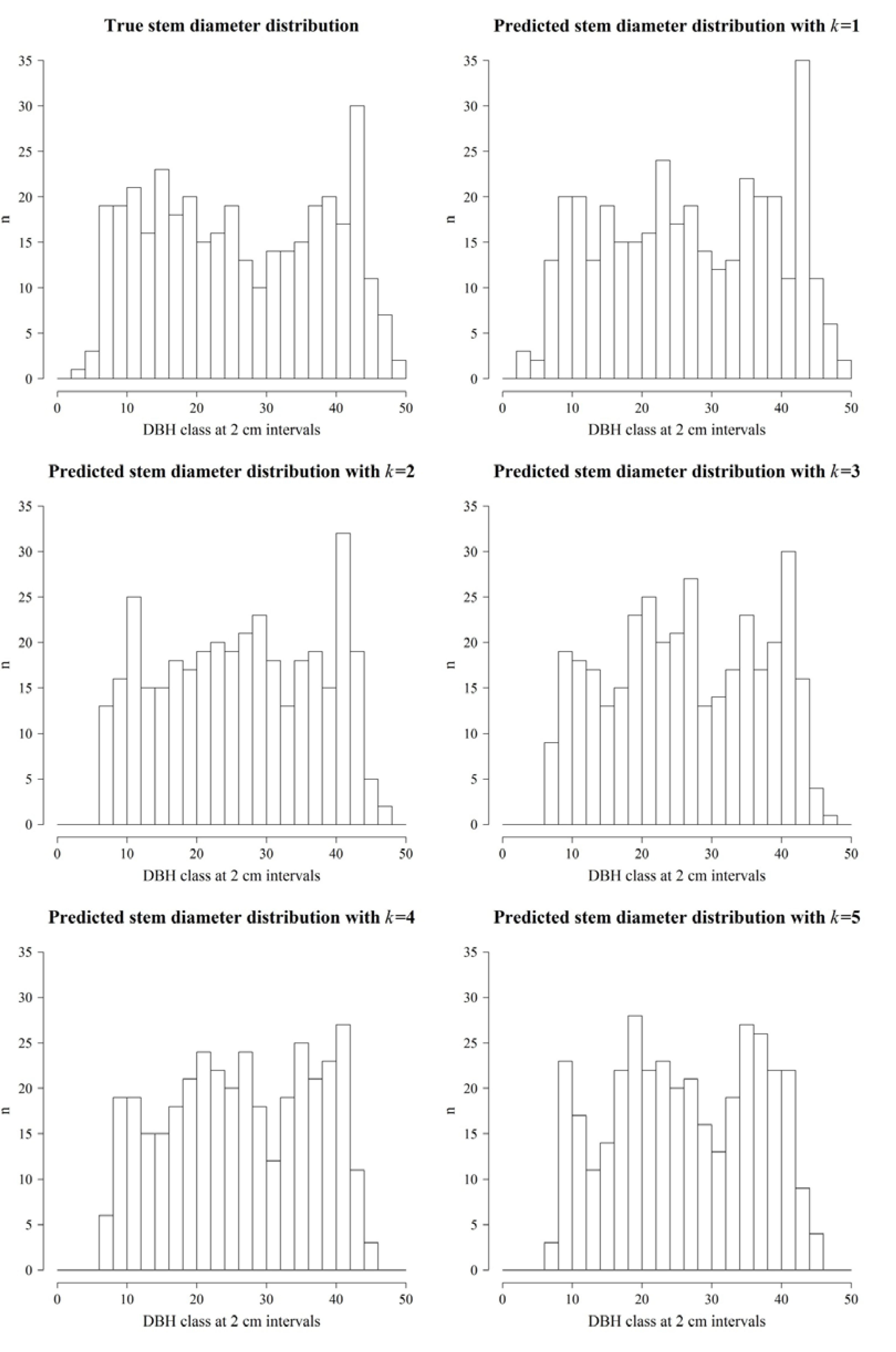
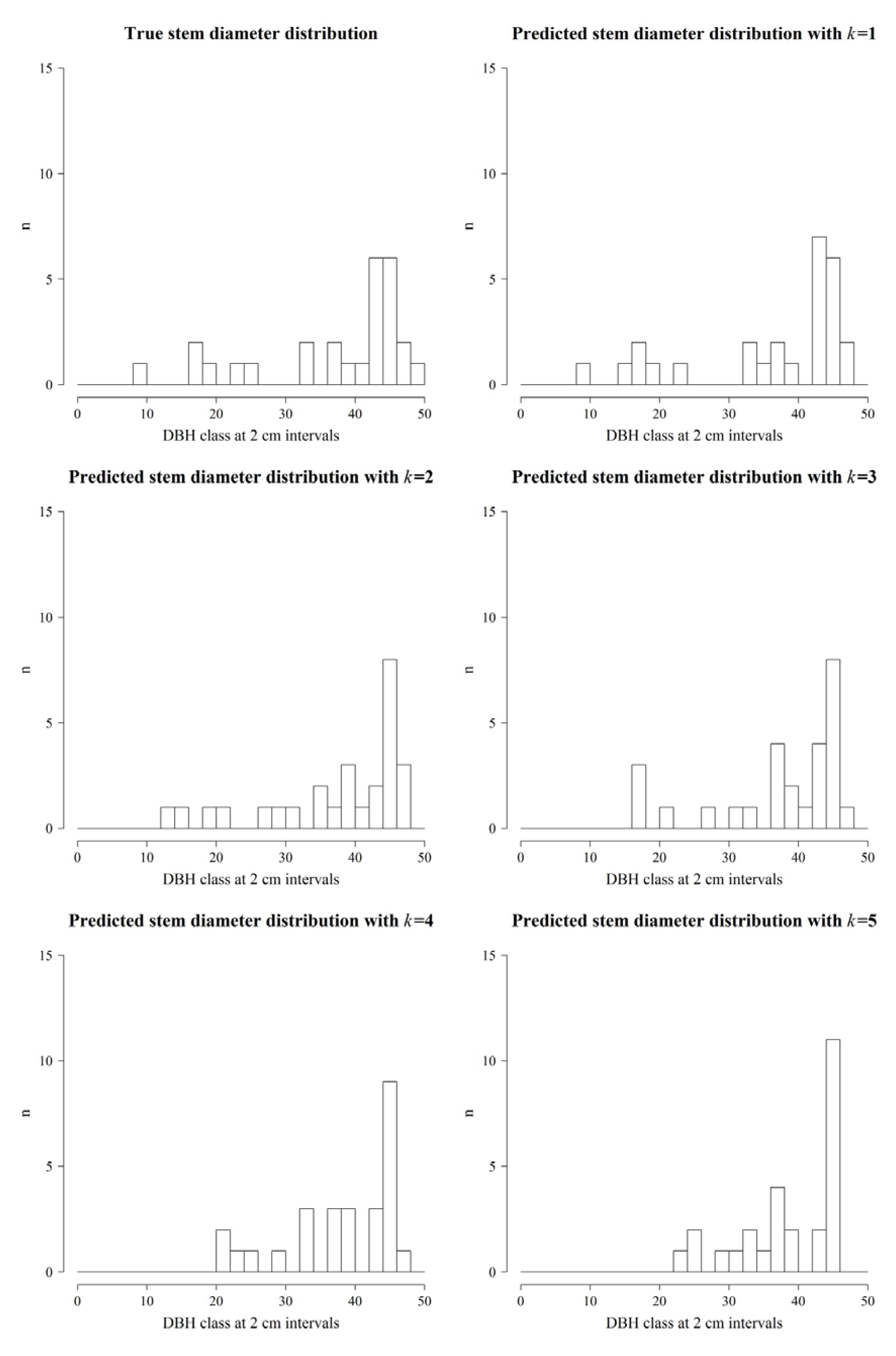
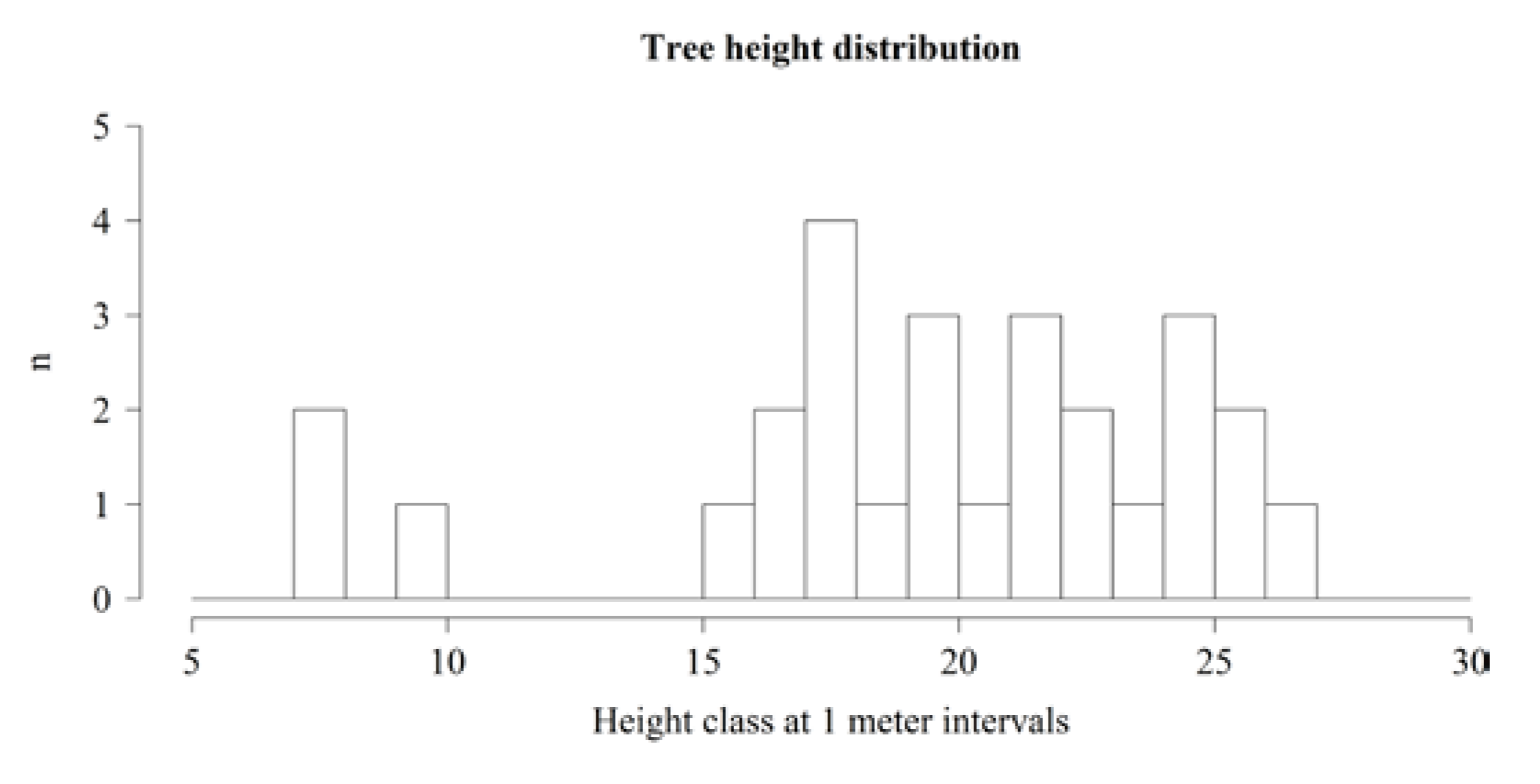
4.3. Comparison of Stem-Distribution Series


| Number of Neighbors | Forest | Park | ||
|---|---|---|---|---|
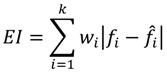
| Error Index | Error Index Using Relative Stem Frequency | Error Index | Error Index Using Relative Stem Frequency | |
| k = 1 | 70 | 0.10 | 6 | 0.11 |
| k = 2 | 110 | 0.15 | 26 | 0.48 |
| k = 3 | 122 | 0.17 | 18 | 0.33 |
| k = 4 | 132 | 0.18 | 20 | 0.37 |
| k = 5 | 152 | 0.21 | 24 | 0.44 |
4.4. Extraction of Tree Height and Crown Area

5. Discussion
6. Conclusions
Acknowledgments
Author Contributions
Conflicts of Interest
References
- Tyrväinen, L.; Pauleit, S.; Seeland, K.; Vries, S. Benefits and uses of urban forests and trees. In Urban Forests and Trees; Konijnendijk, C., Nilsson, K., Randrup, T., Schipperijn, J., Eds.; Springer: Berlin/Heidelberg, Germany, 2005; pp. 81–114. [Google Scholar]
- Beckett, K.P.; Freer-Smith, P.; Taylor, G. Urban woodlands: Their role in reducing the effects of particulate pollution. Environ. Pollut. 1998, 99, 347–360. [Google Scholar] [CrossRef]
- Nowak, D.J. Institutionalizing urban forestry as a “biotechnology” to improve environmental quality. Urban For. Urban Green. 2006, 5, 93–100. [Google Scholar] [CrossRef]
- Zhao, M.; Kong, Z.-H.; Escobedo, F.J.; Gao, J. Impacts of urban forests on offsetting carbon emissions from industrial energy use in Hangzhou, China. J. Environ. Manag. 2010, 91, 807–813. [Google Scholar] [CrossRef]
- Nowak, D.J.; Stevens, J.C.; Sisinni, S.M.; Luley, C.J. Effects of urban tree management and species selection on atmospheric carbon dioxide. J. Arboric. 2002, 28, 113–122. [Google Scholar]
- Arnberger, A. Recreation use of urban forests: An inter-area comparison. Urban For. Urban Green. 2006, 4, 135–144. [Google Scholar] [CrossRef]
- Van Herzele, A.; De Clercq, E.M.; Wiedemann, T. Strategic planning for new woodlands in the urban periphery: Through the lens of social inclusiveness. Urban For. Urban Green. 2005, 3, 177–188. [Google Scholar] [CrossRef]
- Miller, R.W. Urban Forestry: Planning and Managing Urban Greenspaces; Prentice Hall: Upper Saddle River, NJ, USA, 1988. [Google Scholar]
- Rydberg, D.; Falck, J. Urban forestry in Sweden from a silvicultural perspective: A review. Landsc. Urban Plan. 2000, 47, 1–18. [Google Scholar] [CrossRef]
- Zhou, G.; Song, C.; Simmers, J.; Cheng, P. Urban 3D GIS from LiDAR and digital aerial images. Comput. Geosci. 2004, 30, 345–353. [Google Scholar] [CrossRef]
- Næsset, E. Predicting forest stand characteristics with airborne scanning laser using a practical two-stage procedure and field data. Remote Sens. Environ. 2002, 80, 88–99. [Google Scholar] [CrossRef]
- Hyyppä, J.; Inkinen, M. Detecting and estimating attributes for single trees using laser scanner. Photogramm. J. Finl. 1999, 16, 27–42. [Google Scholar]
- Falkowski, M.J.; Smith, A.M.; Gessler, P.E.; Hudak, A.T.; Vierling, L.A.; Evans, J.S. The influence of conifer forest canopy cover on the accuracy of two individual tree measurement algorithms using LiDAR data. Can. J. Remote Sens. 2008, 34, S338–S350. [Google Scholar] [CrossRef]
- Magnussen, S.; Eggermont, P.; LaRiccia, V.N. Recovering tree heights from airborne laser scanner data. For. Sci. 1999, 45, 407–422. [Google Scholar]
- Maltamo, M.; Mustonen, K.; Hyyppä, J.; Pitkänen, J.; Yu, X. The accuracy of estimating individual tree variables with airborne laser scanning in a boreal nature reserve. Can. J. For. Res. 2004, 34, 1791–1801. [Google Scholar] [CrossRef]
- Hyyppa, J.; Kelle, O.; Lehikoinen, M.; Inkinen, M. A segmentation-based method to retrieve stem volume estimates from 3-D tree height models produced by laser scanners. IEEE Trans. Geosci. Remote Sens. 2001, 39, 969–975. [Google Scholar] [CrossRef]
- Naesset, E. Determination of mean tree height of forest stands using airborne laser scanner data. ISPRS J. Photogramm. Remote Sens. 1997, 52, 49–56. [Google Scholar] [CrossRef]
- Wallerman, J.; Holmgren, J. Estimating field-plot data of forest stands using airborne laser scanning and SPOT HRG data. Remote Sens. Environ. 2007, 110, 501–508. [Google Scholar] [CrossRef]
- Vastaranta, M.; Wulder, M.A.; White, J.C.; Pekkarinen, A.; Tuominen, S.; Ginzler, C.; Kankare, V.; Holopainen, M.; Hyyppä, J.; Hyyppä, H. Airborne laser scanning and digital stereo imagery measures of forest structure: Comparative results and implications to forest mapping and inventory update. Can. J. Remote Sens. 2013, 39, 1–14. [Google Scholar] [CrossRef]
- Kankare, V.; Vastaranta, M.; Holopainen, M.; Räty, M.; Yu, X.; Hyyppä, J.; Hyyppä, H.; Alho, P.; Viitala, R. Retrieval of forest aboveground biomass and stem volume with airborne scanning LiDAR. Remote Sens. 2013, 5, 2257–2274. [Google Scholar] [CrossRef] [Green Version]
- Lefsky, M.A.; Harding, D.; Cohen, W.; Parker, G.; Shugart, H. Surface LiDAR remote sensing of basal area and biomass in deciduous forests of eastern Maryland, USA. Remote Sens. Environ. 1999, 67, 83–98. [Google Scholar] [CrossRef]
- Means, J.E.; Acker, S.A.; Fitt, B.J.; Renslow, M.; Emerson, L.; Hendrix, C.J. Predicting forest stand characteristics with airborne scanning LiDAR. Photogramm. Eng. Remote Sens. 2000, 66, 1367–1372. [Google Scholar]
- Brandtberg, T. Classifying individual tree species under leaf-off and leaf-on conditions using airborne LiDAR. ISPRS J. Photogramm. Remote Sens. 2007, 61, 325–340. [Google Scholar] [CrossRef]
- Holmgren, J.; Persson, Å. Identifying species of individual trees using airborne laser scanner. Remote Sens. Environ. 2004, 90, 415–423. [Google Scholar] [CrossRef]
- Korpela, I.; Ørka, H.O.; Maltamo, M.; Tokola, T.; Hyyppä, J. Tree species classification using airborne LiDAR—Effects of stand and tree parameters, downsizing of training set, intensity normalization, and sensor type. Silva Fenn. 2010, 44, 319–339. [Google Scholar]
- Van Aardt, J.A.; Wynne, R.H.; Scrivani, J.A. LiDAR-based mapping of forest volume and biomass by taxonomic group using structurally homogenous segments. Photogramm. Eng. Remote Sens. 2008, 74, 1033–1044. [Google Scholar] [CrossRef]
- Vauhkonen, J.; Korpela, I.; Maltamo, M.; Tokola, T. Imputation of single-tree attributes using airborne laser scanning-based height, intensity, and alpha shape metrics. Remote Sens. Environ. 2010, 114, 1263–1276. [Google Scholar] [CrossRef]
- Maas, H.G.; Bienert, A.; Scheller, S.; Keane, E. Automatic forest inventory parameter determination from terrestrial laser scanner data. Int. J. Remote Sens. 2008, 29, 1579–1593. [Google Scholar] [CrossRef]
- Moskal, L.M.; Zheng, G. Retrieving forest inventory variables with Terrestrial Laser Scanning (TLS) in urban heterogeneous forest. Remote Sens. 2011, 4, 1–20. [Google Scholar] [CrossRef]
- Vastaranta, M.; Melkas, T.; Holopainen, M.; Kaartinen, H.; Hyyppä, J.; Hyyppä, H. Comparison of different laser-based methods to measure stem diameter. In Proceedings of the SilviLaser 2008, the 8th International Conference on LiDAR Applications in Forest Assessment and Inventory, Edinburgh, UK, 17–19 September 2008.
- Holopainen, M.; Kankare, V.; Vastaranta, M.; Liang, X.; Lin, Y.; Vaaja, M.; Yu, X.; Hyyppä, J.; Hyyppä, H.; Kaartinen, H. Tree mapping using airborne, terrestrial and mobile laser scanning—A case study in a heterogeneous urban forest. Urban For. Urban Green. 2013, 12, 546–553. [Google Scholar]
- Holopainen, M.; Vastaranta, M.; Kankare, V.; Hyyppä, J.; Liang, X.; Litkey, P.; Yu, X.; Kaartinen, H.; Kukko, A.; Kaasalainen, S. The use of ALS, TLS and VLS measurements in mapping and monitoring urban trees. In Proceedings of the 2011 Joint Urban Remote Sensing Event (JURSE), Munich, Germany, 11–13 April 2011; pp. 29–32.
- Liang, X.; Litkey, P.; Hyyppä, J.; Kaartinen, H.; Vastaranta, M.; Holopainen, M. Automatic stem mapping using single-scan terrestrial laser scanning. IEEE Trans. Geosci. Remote Sens. 2012, 50, 661–670. [Google Scholar] [CrossRef]
- Liang, X.; Hyyppä, J.; Kankare, V.; Holopainen, M. Stem curve measurement using terrestrial laser scanning. In Proceedings of the 11th International Conference on LiDAR Applications for Assessing Forest Ecosystems, Hobart, Australia, 16–19 October, 2011; pp. 1–6.
- Liang, X.; Kankare, V.; Yu, X.; Hyyppä, J.; Holopainen, M. Automated stem curve measurement using terrestrial laser scanning. IEEE Trans. Geosci. Remote Sens. 2013, 52, 1739–1748. [Google Scholar]
- Pfeifer, N.; Winterhalder, D. Modelling of tree cross sections from terrestrial laser scanning data with free-form curves. Int. Arch. Photogramm. Remote Sens. Spat. Inf. Sci. 2004, 36, part2/W2. 76–81. [Google Scholar]
- Hyyppa, J.; Jaakkola, A.; Hyyppa, H.; Kaartinen, H.; Kukko, A.; Holopainen, M.; Zhu, L.; Vastaranta, M.; Kaasalainen, S.; Krooks, A. Map updating and change detection using vehicle-based laser scanning. In Proceedings of the 2009 Joint Urban Remote Sensing Event, Shanghai, China, 20–22 May 2009; pp. 1–6.
- Kaasalainen, S.; Hyyppä, J.; Karjalainen, M.; Krooks, A.; Lyytikäinen-Saarenmaa, P.; Holopainen, M.; Jaakkola, A. Comparison of terrestrial laser scanner and synthetic aperture radar data in the study of forest defoliation. Int. Arch. Photogramm. Remote Sens. Spat. Inf. Sci. 2010, 38, 82–87. [Google Scholar]
- Kankare, V.; Holopainen, M.; Vastaranta, M.; Puttonen, E.; Yu, X.W.; Hyyppa, J.; Vaaja, M.; Hyyppa, H.; Alho, P. Individual tree biomass estimation using terrestrial laser scanning. ISPRS J. Photogramm. Remote Sens. 2013, 75, 64–75. [Google Scholar] [CrossRef]
- Yao, T.; Yang, X.; Zhao, F.; Wang, Z.; Zhang, Q.; Jupp, D.; Lovell, J.; Culvenor, D.; Newnham, G.; Ni-Meister, W. Measuring forest structure and biomass in New England forest stands using Echidna ground-based lidar. Remote Sens. Environ. 2011, 115, 2965–2974. [Google Scholar] [CrossRef]
- Yu, X.W.; Liang, X.L.; Hyyppa, J.; Kankare, V.; Vastaranta, M.; Holopainen, M. Stem biomass estimation based on stem reconstruction from terrestrial laser scanning point clouds. Remote Sens. Lett. 2013, 4, 344–353. [Google Scholar] [CrossRef]
- Zhao, F.; Yang, X.; Schull, M.A.; Román-Colón, M.O.; Yao, T.; Wang, Z.; Zhang, Q.; Jupp, D.L.; Lovell, J.L.; Culvenor, D.S. Measuring effective leaf area index, foliage profile, and stand height in New England forest stands using a full-waveform ground-based lidar. Remote Sens. Environ. 2011, 115, 2954–2964. [Google Scholar] [CrossRef]
- Tanhuanpää, T.V.; Vastaranta, M.; Kankare, V.; Holopainen, M.; Hyyppä, J.; Hyyppä, H.; Alho, P.; Raisio, J. Mapping of urban roadside trees—A case study in the tree register update process in helsinki city. Urban For. Urban Green. 2014, 13. [Google Scholar] [CrossRef]
- Holopainen, M.H.; Hyyppä, J.; Vastaranta, M.; Hyyppä, H. Laserkeilaus Metsävarojen Hallinnassa; University of Helsinki Department of Forest Sciences: Helsinki, Finland, 2013; Volume 5, p. 75. [Google Scholar]
- Axelsson, P. DEM generation from laser scanner data using adaptive tin models. Int. Arch. Photogramm. Remote Sens. 2000, 33, 111–118. [Google Scholar]
- Vastaranta, M.; Kankare, V.; Holopainen, M.; Yu, X.; Hyyppä, J.; Hyyppä, H. Combination of individual tree detection and area-based approach in imputation of forest variables using airborne laser data. ISPRS J. Photogramm. Remote Sens. 2012, 67, 73–79. [Google Scholar] [CrossRef]
- Yu, X.; Hyyppä, J.; Vastaranta, M.; Holopainen, M.; Viitala, R. Predicting individual tree attributes from airborne laser point clouds based on the random forests technique. ISPRS J. Photogramm. Remote Sens. 2011, 66, 28–37. [Google Scholar] [CrossRef]
- Breiman, L. Random forests. Mach. Learn. 2001, 45, 5–32. [Google Scholar] [CrossRef]
- Falkowski, M.J.; Hudak, A.T.; Crookston, N.L.; Gessler, P.E.; Uebler, E.H.; Smith, A.M. Landscape-scale parameterization of a tree-level forest growth model: A k-nearest neighbor imputation approach incorporating LiDAR data. Can. J. For. Res. 2010, 40, 184–199. [Google Scholar] [CrossRef]
- Hudak, A.T.; Crookston, N.L.; Evans, J.S.; Hall, D.E.; Falkowski, M.J. Nearest neighbor imputation of species-level, plot-scale forest structure attributes from LiDAR data. Remote Sens. Environ. 2008, 112, 2232–2245. [Google Scholar]
- Latifi, H.; Nothdurft, A.; Koch, B. Non-parametric prediction and mapping of standing timber volume and biomass in a temperate forest: Application of multiple optical/LiDAR-derived predictors. Forestry 2010, 83, 395–407. [Google Scholar] [CrossRef]
- Team, R.D.C. R: A Language and Environment for Statistical Computing; R Foundation for Statistical Computing: Vienna, Austria, 2013. Available online: http://www.R-project.org (accessed on 2 December 2013).
- Crookston, N.L.; Finley, A.O. Yaimpute: An R Package for kNN imputation. J. Stat. Softw. 2008, 23, 1–16. [Google Scholar]
- Reynolds, M.R.; Burk, T.E.; Huang, W.-C. Goodness-of-fit tests and model selection procedures for diameter distribution models. For. Sci. 1988, 34, 373–399. [Google Scholar]
- Packalén, P.; Maltamo, M. Estimation of species-specific diameter distributions using airborne laser scanning and aerial photographs. Can. J. For. Res. 2008, 38, 1750–1760. [Google Scholar] [CrossRef]
- Holmgren, J.; Barth, A.; Larsson, H.; Olsson, H. Prediction of stem attributes by combining airborne laser scanning and measurements from harvesters. Silva Fenn. 2012, 46, 227–239. [Google Scholar]
- Maltamo, M.; Peuhkurinen, J.; Malinen, J.; Vauhkonen, J.; Packalén, P.; Tokola, T. Predicting tree attributes and quality characteristics of scots pine using airborne laser scanning data. Silva Fenn. 2009, 43, 507–521. [Google Scholar]
- Peuhkurinen, J.; Maltamo, M.; Malinen, J.; Pitkanen, J.; Packalen, P. Preharvest measurement of marked stands using airborne laser scanning. For. Sci. 2007, 53, 653–661. [Google Scholar]
- Kaartinen, H.; Hyyppä, J.; Yu, X.; Vastaranta, M.; Hyyppä, H.; Kukko, A.; Holopainen, M.; Heipke, C.; Hirschmugl, M.; Morsdorf, F. An international comparison of individual tree detection and extraction using airborne laser scanning. Remote Sens. 2012, 4, 950–974. [Google Scholar] [CrossRef] [Green Version]
- Pitkänen, J.; Maltamo, M.; Hyyppä, J.; Yu, X. Adaptive methods for individual tree detection on airborne laser based canopy height model. Int. Arch. Photogramm. Remote Sens. Spat. Inf. Sci. 2004, 36, 187–191. [Google Scholar]
- Vauhkonen, J.; Ene, L.; Gupta, S.; Heinzel, J.; Holmgren, J.; Pitkänen, J.; Solberg, S.; Wang, Y.; Weinacker, H.; Hauglin, K.M. Comparative testing of single-tree detection algorithms under different types of forest. Forestry 2012, 85, 27–40. [Google Scholar] [CrossRef]
- Forsman, P.; Halme, A. 3-D mapping of natural environments with trees by means of mobile perception. IEEE Trans. Robot. 2005, 21, 482–490. [Google Scholar] [CrossRef]
- Hellström, T.; Lärkeryd, P.; Nordfjell, T.; Ringdahl, O. Autonomous forest vehicles: Historic, envisioned, and state-of-the-art. Int. J. For. Eng. 2009, 20, 31–38. [Google Scholar]
- Jutila, J.; Kannas, K.; Visala, A. Tree measurement in forest by 2D laser scanning. In Proceedings of the International Symposium on Computational Intelligence in Robotics and AutomationCIRA 2007, Jacksonville, FI, USA, 20–23 June 2007; pp. 491–496.
- Miettinen, M.; Ohman, M.; Visala, A.; Forsman, P. Simultaneous localization and mapping for forest harvesters. In Proceedings of the 2007 IEEE International Conference on Robotics and Automation, Roma, Romania, 10–14 April 2007; pp. 517–522.
- Ringdahl, O.; Hohnloser, P.; Hellström, T.; Holmgren, J.; Lindroos, O. Enhanced algorithms for estimating tree trunk diameter using 2D laser scanner. Remote Sens. 2013, 5, 4839–4856. [Google Scholar] [CrossRef]
- Öhman, M.; Miettinen, M.; Kannas, K.; Jutila, J.; Visala, A.; Forsman, P. Tree measurement and simultaneous localization and mapping system for forest harvesters. In Field and Service Robotics; Springer-Verlag: Berlin/Heidelberg, Germany, 2008; pp. 369–378. [Google Scholar]
- Lindberg, E.; Holmgren, J.; Olofsson, K.; Olsson, H. Estimation of stem attributes using a combination of terrestrial and airborne laser scanning. Eur. J. For. Res. 2012, 131, 1917–1931. [Google Scholar] [CrossRef]
- Vauhkonen, J.; Packalen, P.; Malinen, J.; Pitkänen, J.; Maltamo, M. Airborne laser scanning based decision support for wood procurement planning. Scand. J. For. Res. 2013, 28. [Google Scholar] [CrossRef]
- Rönnholm, P.; Hyyppä, J.; Hyyppä, H.; Haggrén, H.; Yu, X.; Kaartinen, H. Calibration of laser-derived tree height estimates by means of photogrammetric techniques. Scand. J. For. Res. 2004, 19, 524–528. [Google Scholar] [CrossRef]
- Shrestha, R.; Wynne, R.H. Estimating biophysical parameters of individual trees in an urban environment using small footprint discrete-return imaging LiDAR. Remote Sens. 2012, 4, 484–508. [Google Scholar] [CrossRef]
- Vastaranta, M.; Melkas, T.; Holopainen, M.; Kaartinen, H.; Hyyppä, J.; Hyyppä, H. Laser-based field measurements in tree-level forest data acquisition. Photogramm. J. Finl. 2009, 21, 51–61. [Google Scholar]
© 2014 by the authors; licensee MDPI, Basel, Switzerland. This article is an open access article distributed under the terms and conditions of the Creative Commons Attribution license (http://creativecommons.org/licenses/by/3.0/).
Share and Cite
Saarinen, N.; Vastaranta, M.; Kankare, V.; Tanhuanpää, T.; Holopainen, M.; Hyyppä, J.; Hyyppä, H. Urban-Tree-Attribute Update Using Multisource Single-Tree Inventory. Forests 2014, 5, 1032-1052. https://doi.org/10.3390/f5051032
Saarinen N, Vastaranta M, Kankare V, Tanhuanpää T, Holopainen M, Hyyppä J, Hyyppä H. Urban-Tree-Attribute Update Using Multisource Single-Tree Inventory. Forests. 2014; 5(5):1032-1052. https://doi.org/10.3390/f5051032
Chicago/Turabian StyleSaarinen, Ninni, Mikko Vastaranta, Ville Kankare, Topi Tanhuanpää, Markus Holopainen, Juha Hyyppä, and Hannu Hyyppä. 2014. "Urban-Tree-Attribute Update Using Multisource Single-Tree Inventory" Forests 5, no. 5: 1032-1052. https://doi.org/10.3390/f5051032
APA StyleSaarinen, N., Vastaranta, M., Kankare, V., Tanhuanpää, T., Holopainen, M., Hyyppä, J., & Hyyppä, H. (2014). Urban-Tree-Attribute Update Using Multisource Single-Tree Inventory. Forests, 5(5), 1032-1052. https://doi.org/10.3390/f5051032