Article

Classification of Needle Loss of Individual Scots Pine Trees by Means of Airborne Laser Scanning

1
Department of Forest Sciences, University of Helsinki, P.O. Box 27, Helsinki FI-00014, Finland
2
Department of Remote Sensing and Photogrammetry, Finnish Geodetic Institute, Masala FI-02431, Finland
*
Author to whom correspondence should be addressed.
Forests 2013, 4(2), 386-403; https://doi.org/10.3390/f4020386
Submission received: 1 April 2013 / Revised: 23 May 2013 / Accepted: 27 May 2013 / Published: 14 June 2013

Abstract

:
Forest disturbances caused by pest insects are threatening ecosystem stability, sustainable forest management and economic return in boreal forests. Climate change and increased extreme weather patterns can magnify the intensity of forest disturbances, particularly at higher latitudes. Due to rapid responses to elevating temperatures, forest insect pests can flexibly change their survival, dispersal and geographic distributions. The outbreak pattern of forest pests in Finland has evidently changed during the last decade. Projection of shifts in distributions of insect-caused forest damages has become a critical issue in the field of forest research. The Common pine sawfly (Diprion pini L.) (Hymenoptera, Diprionidae) is regarded as a significant threat to boreal pine forests. Defoliation by D. pini has resulted in severe growth loss and mortality of Scots pine (Pinus sylvestris L.) (Pinaceae) in eastern Finland. In this study, tree-wise defoliation was estimated for five different needle loss category classification schemes and for 10 different simulated airborne laser scanning (ALS) pulse densities. The nearest neighbor (NN) approach, a nonparametric estimation method, was used for estimating needle loss of 701 Scots pines, using the means of individual tree features derived from ALS data. The Random Forest (RF) method was applied in NN-search. For the full dense data (~20 pulses/m2), the overall estimation accuracies for tree-wise defoliation level varied between 71.0% and 86.5% (kappa-values of 0.56 and 0.57, respectively), depending on the classification scheme. The overall classification accuracies for two class estimation with different ALS pulse densities varied between 82.8% and 83.7% (kappa-values of 0.62 and 0.67, respectively). We conclude that ALS-based estimation of needle losses may be of acceptable accuracy for individual trees. Our method did not appear sensitive to the applied pulse densities.

1. Introduction

Boreal forest ecosystems normally are highly dynamic and resilient to a variety of changes which promotes stable development of forest stands across broad temporal and spatial scales. Normal variations in annual growth patterns and needle biomass need to be distinguished from disturbances leading to declining forest health. Disturbance interrupts successional development of forest ecosystems, affecting resources, the physical environment, population structure, and, in extreme cases, changing the direction of successional processes [1,2]. Forest disturbances can appear in different forms such as abiotic (storm, drought, frost, snow, fire) or biotic (pest insects, diseases, mammals) damages [3,4], causing threats to sustainable forest management and economic return in the Boreal Zone [5,6].
Climate change and increased extreme weather patterns can magnify the intensity of forest disturbances, altering the geographical range and productivity of forests, especially at higher latitudes [7,8,9]. During global warming, increases in stress factors and patterns of insect outbreaks have been predicted [8,9,10,11,12]. Due to rapid responses to elevating temperatures, pest insects can flexibly change their survival, development, reproduction, dispersal and geographic distribution [13,14,15,16]. Increasing numbers of pest insects have already begun to expand their normal geographic ranges, either pole-ward latitudinally or upward altitudinally [17,18,19], or change their pest status within their ranges [20]. Increased outbreak frequencies and spatial scales of forest pests evidently have already undergone changes during the most recent decade in Finland, particularly with pine sawflies [20].
Development of modern, cost-efficient monitoring methods for forest sites affected by climate-driven disturbance agents is urgently needed [21]. Monitoring of needle defoliation has typically been based on field sampling [22], which consumes vast resources, only to yield results that may still be biased. Furthermore, estimates of future defoliation and yield losses are only qualitative. The Finnish Forest Research Institute carries out the National Forest Inventory (NFI) [23], in which information on forest health is collected as a side product and monitored on a coarse level. The annual requirements of precise information on forest disturbances are not met by the current practice of forest health monitoring.
Remote sensing is an efficient tool for detecting changes in forested areas, such as disturbances [24]. Current development in active remote sensing technologies, especially airborne laser scanning (ALS) techniques have resulted in new methods for carrying out various forest inventory tasks. With the capability of direct or derived measurement of forest structure, including canopy height, crown dimensions and above-ground biomass, ALS can be also applied for monitoring of forest hazards. Previous studies have shown that ALS data can be used to estimate several forest inventory attributes, such as the tree-, plot- and stand-level characteristics of tree height [25,26,27], biomass [27,28,29,30], volume [31,32], basal area [33,34], tree species [29,35,36] and forest operations [37,38]. ALS can be useful in projecting, detecting and monitoring forest hazards and tree defoliation due to its ability to directly measure vegetation structure [39,40,41]. Recent studies and developments in methods have achieved more accurate ALS-based biomass detection [39,42,43,44,45,46,47,48]. Single trees biomass and defoliation level are highly correlated (e.g., [49]).
The objective of this present study was to test the accuracy in tree-wise classification of needle defoliation after consumption by pine sawflies over a period of several years in a row. Defoliation estimations were made using several needle loss category classification schemes, in order to investigate their effects on accuracy. Classifications were based upon statistical metrics extracted from ALS data at the level of a single tree crown. The hypothesis was that the distribution of laser returns from defoliated trees differs from that of healthy, undefoliated trees. Kantola et al. [39] earlier investigated how to separate healthy and severely defoliated trees using an approach similar to that used here combining ALS data with high resolution aerial imagery. Vastaranta et al. [48] developed an area-based approach for mapping healthy and defoliated Scots pine stands with ALS data. In both of these studies, simple two-class defoliation classification schemes were used. This study included multiple higher level defoliation classification schemes in order to extract more detailed information. An additional objective involved determining the effect of laser pulse density on the classification accuracy.

2. Material and Methods

2.1. Study Area

The research site was in Ilomantsi, eastern Finland (62°53′N, 30°54′E) (Figure 1). The 34.5 km2 wide study area covers mainly dry or dryish forest site types in soils consisting of a combination of silt, sand and gravel. The main forest types in the Palokangas study area are Calluna (CT type), Vaccinium (VT type) and Myrtillus (MT type) [50]. The relief is flat at a mean altitude of 170 m, gently rolling towards the northern edge of the area. The dominance of Scots pine (Pinus sylvestris L.) (Pinacea) was 99.5% in this commercial forest. The majority of stands were young or middle-aged, having a mean age of 53 years and mean diameter-at-breast-height (dbh) of 14.7 cm.
The initial outbreak of the common pine sawfly (Diprion pini L.) was first visible in 1999 in the area. Outbreak range, population density and damage intensity have fluctuated over the last 12 years, indicating a chronic nature. Due to a feeding pattern of D. pini, i.e., consumption of all the needle year-classes in August and September, the pest has caused vast damage and tree mortality in an area of approximately 10,000 ha. The forest owner has carried out large cuttings due to activity of this insect pest.
Figure 1. Location of the study area (left, ESRI©) and map with tree locations (red) and forest compartments. (Green colors indicates different site types, 2 = grove-like heath, 3 = fresh heath, 4 = dryish heath, 5 = dry heath and 6 = barren heath)
Forests 04 00386 g001

2.2. Airborne Laser Scanning Data Set

The ALS data set was from October 2008 and acquired with a Leica ALS50-II SN058 laser scanner (Leica Geosystem AG, Heerbrugg, Switzerland). The flying altitude was 500 m at a speed of 80 knots, with a field of view of 30 degrees, pulse rate of 150 kHz, scanning rate of 52 Hz, and a ground level laser footprint size of 0.11 m. The density of the pulses returned within the field plots was approximately 20 pulses per m2. ALS data was classified to ground and non-ground returns using the standard TerraScan approach described by Axelsson [51]. A digital elevation model (DEM) was created using classified ground pulses. Laser heights above ground (normalized height or canopy height) were calculated by subtracting the ground elevation from corresponding laser measurements.

2.3. Reference Data

2.3.1. Field Measurements

Field measurements were carried out in May and early June 2009 before elongation of the current season’s needles, representing the defoliation status of fall 2008. Adaptive cluster sampling (ACS) was applied as an inventory method [52]. In ACS, an initial set of sampling plots is selected using a simple probability sampling procedure. Additional sampling plots from the neighborhood are added, where the variable of interest (i.e., plot-wise defoliation) satisfied a given criterion [48]. This procedure is repeated until no additional plots could be found. According to Thompson [53], Roesch [54] and Talvitie et al. [52], ACS has an advantage over more conventional sampling methods used in forest inventory for sampling rare and clustered phenomena. The sampling efforts are focused on areas with high numbers of variables of interest. The sampling plot centers were located with a Trimble Pro XH (Trimble Navigation Ltd., Sunnyvale, CA, USA), which can reach up to 30 cm precision with differential postprocessing. Each individual tree was located by measuring the distance and angle from the plot center to the tree. The visual assessment of defoliation intensity was performed simultaneously with tree wise measurements in the field sampling plots. The defoliation intensity of a single tree was visually assessed from different directions, according to Eichhorn [55], comparing the amount of needles of the tree to an imaginary reference tree with full healthy foliage growing in the same forest type. An accuracy of 10% was assigned to the visual assessment of needle loss.

2.3.2. Tree Detection and Linking of ALS and Field Data

Individual tree detection (ITD) was done from the smoothened 0.5 m grid canopy height model (CHM) using watershed segmentation. (For more detailed description of tree delineation, see [56,57].) The resulting ITD segments and the trees measured in the field were verified and data sets were combined. 701 segments were considered as single Scots pine crowns. The segments that included more than one field tree were removed from the data, due to the confounding of different needle loss levels among the various trees aligning into same segment. In most cases where segments had more than one tree, the tree crowns were notably overlapping with one or more trees originating from the suppressed canopy cover layer. Most of the Scots pines suffered from mild to moderate defoliation (10%–30%) (Table 1). Only 55 of the identified trees had a defoliation level of 40% or more.
Table 1. Field tree measurement data, where dbh is the measured diameter-at-breast height (cm), h is the height of a tree (m) (a) and defoliation assessment (0%–100%) is the estimated needle loss in the field (b).
(a)(b)
minmaxmeansdDefoliation (%)Number of trees
dbh (cm)5340522213043
h (m)8.626.218.83.110222
20266
30115
4036
50–10019
Total701

2.3.3. Classification Schemes for Defoliation

The data was divided into five different classification schemes for testing classification accuracy at different coarseness levels. The number of defoliation classes in different combinations varied between two and four threshold values (Table 2). Those trees having a lower defoliation intensity value than the threshold value of the class fell into a lower class. Classification DEF1 (two classes with threshold value of 20% of defoliation) was used as a basis of all other calculations due to 20% of defoliation being considered as the threshold value for a significant needle loss.
Table 2. The five different classification schemes with threshold values and number of classes in every scheme.
ClassificationThreshold defoliation levelsClasses (n)
DEF120%2
DEF230%2
DEF330%, 60%3
DEF420%, 50%3
DEF520%, 30%, 40%4

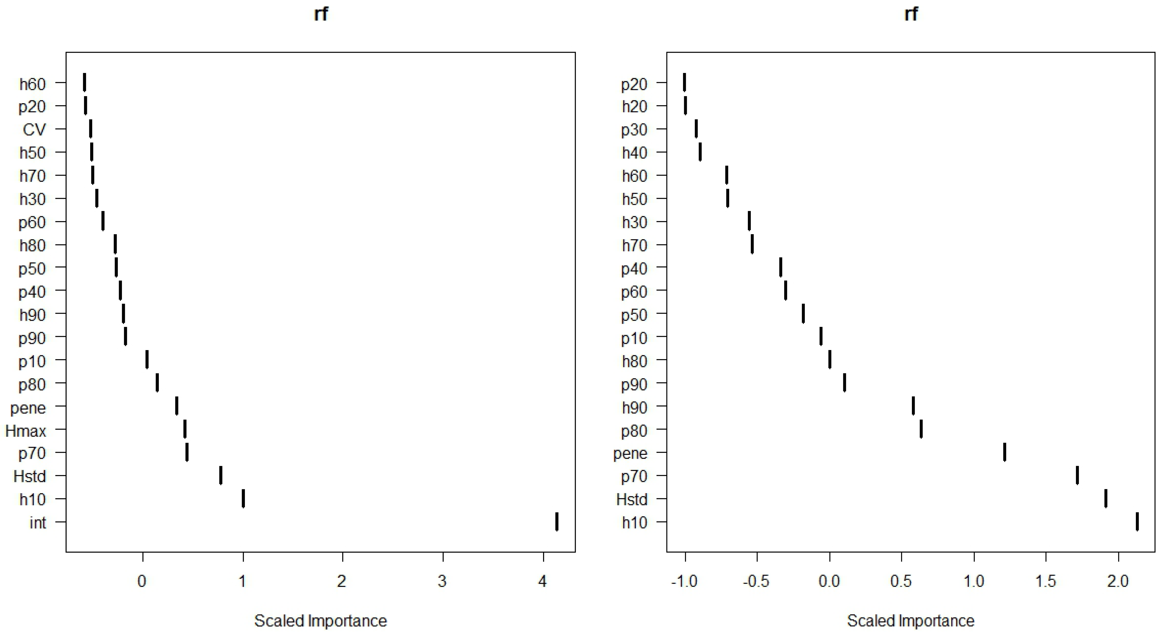
2.4. ALS Feature Extraction

Laser returns falling within each individual tree segment were extracted and the canopy heights of these returns were used to derive the ALS features for each tree. The “first” and “only” returns were chosen for this analysis because they have the highest reflections, and are less affected by intra-crown transmission losses [30]. Furthermore, the physics behind the interaction between later ALS returns and the forest canopy is more complex. We could have assumed that later returns would have brought valuable information about defoliation, but in reality, there are too many uncertainties in those returns coming after the pulse starts to penetrate into the canopy. For example, later return pulses may have penetrated through a tree that is not within plot, through branches, overlapping crowns or understory vegetation. A total of 26 laser point metrics were calculated from canopy returns. Metrics included maximum (Hmax), mean (Hmean), and standard deviation (Hstd) of heights, 10 height percentiles and proportions of canopy returns at various relative heights (Table 3). Mean return intensity was also calculated.
Table 3. Statistical metrics calculated from airborne laser scanning (ALS) data for individual trees. A total of 10 discrete metrics are included in both h10–h90 and p10–p90.
FeatureDescription
HmaxMaximum height of laser returns
HmeanArithmetic mean of laser heights
HstdStandard deviation of heights
CVHstd divided by Hmean
h10–h90Heights 0th–90th percentile
p10–p90Percentile of canopy height distribution
penePenetration calculated as a proportion of returns below 2 m to total returns
IntMean intensity

2.5. Estimation of Defoliation

The nearest neighbor (NN) approach was used to estimate the defoliation classes of trees. Tree-wise defoliation level determined in the field was used as the target observation (y value) and tree-specific metrics derived from ALS data were used as the predictors (x values). Random Forest (RF) [58] was applied in the NN search. The RF method is explained in detail by Crookston and Finley [59] and Falkowski et al. [60]. Hudak et al. [61] and Latifi et al. [62] showed that the RF method is robust and flexible in forest characteristics prediction compared with other NN methods, favoring the selection of RF for NN searching in this study. In the RF method, several regression or classification trees are generated by drawing a replacement of two thirds of the data for training and one third for testing each tree. A regression tree is a sequence of rules that splits the feature space into partitions having values similar to the response variable. A method based on classification and regression trees (CART) is usually adopted to generate regression trees. At each node of a regression tree, data are split until the leaf nodes contain fewer samples than some preselected value, or the sum of the squares of the distances to the mean value of the respective group is less than the threshold. Measurement of nearness in RF is defined, based on observations of the probability of ending up in the same terminal node during classification. The output is the percent increase in misclassification rate as compared to the out-of-bag rate (with all variables intact). The number of NNs (parameter k) was chosen to be three. In forest variable predictions, stable results are obtained with k values between two and seven, though bias being smallest with k value of one. A total of 2000 regression trees were fitted in each RF run to gain more consistency. In addition calculations RF predictions were repeated 10 times and the overall classification accuracies and kappa-values were calculated as a mean from the results of the RF runs.
RF is increasingly used in various ALS applications such as for classification of forest structure [63] and tree species [30], defoliation [39,48] and for estimation of tree variables [57]. The R yaImpute library [59] was employed in the RF estimations.

2.6. Simulation of Pulse Densities

The availability of dense ALS data (~20 pulses/m2) enabled the simulation of the effects of pulse density on the classification accuracy in mapping of estimated defoliation. The entire set of data was initially used to create individual tree segments and to select the ALS metrics for estimating defoliation. The goal was to assess the effect of the pulse density on classification accuracy rather than to find the best explanatory ALS metrics for different pulse densities or to study the ITD procedure with different pulse densities. The original ALS data was thinned with simple random sampling procedure at 10% intervals and calculations of the ALS metrics and estimations of defoliation were made of the thinned data. Pulse densities of 20, 18, 16, 14, 12, 10, 8, 6, 4, and 2 pulses/m2 were simulated and tested. The thinning, calculation of ALS metrics and classifications were repeated 10 times to provide more stability in the results. Densities coarser than 2 pulses/m2 were not studied since they fell beneath the minimum requirement normally considered for this kind of ITD method (e.g., [64,65]).

3. Results

3.1. Classification of Defoliation

In the first phase, RF was run for the DEF1 classification scheme with all possible classifiers included to obtain the RF scaled importance of ALS metrics. This was justified due to the overall small number of classifiers (26 metrics). Mean return intensity was the most powerful predictor in the first run. In this study, the intensity was not calibrated and hence ruled out. On the basis of field measurements, it could be assumed that dominant trees are commonly more defoliated by D. pini than the dominated trees. In order to classify the defoliation phenomenon and not tree size, the ALS metrics Hmax and Hmean were also eliminated.
RF is considered to be a robust classification method, but the number of explanatory variables was still held low to avoid over-fitting. Over-fitting can occur, especially if used data is very noisy. Based on these preliminary runs, the three most important classifiers were tenth height percentile (h10), standard deviation of heights (Hstd) and seventh percentile of canopy height distribution (p70) (Figure 2). The correlations between the three most important metrics were not strong and difference between distributions of healthy and defoliated trees were found (Table 4). Thus these three ALS metrics were used in all further classifications.
Figure 2. Scaled importance of top 20 ALS metrics in Random Forest (RF) run for classification of defoliation (classification scheme DEF1). All ALS metrics on left and ALS metrics included on right.
Forests 04 00386 g002
Table 4. Pearson’s correlation, mean values for healthy and defoliated trees and significance for explanatory ALS features.
Correlations Mean valuest-Test
Featureh10Hstdp70HealthyDefoliatedp-Value
h101.00−0.34−0.320.18020.9657<0.000
Hstd−0.341.00−0.246.06845.0588<0.000
p70−0.32−0.241.000.53060.51530.19
The overall classification accuracies for defoliation were over 80% for classification schemes having two or three defoliation classes (Table 4). The overall classification accuracies were calculated as a mean of 10 RF runs. The best overall classification accuracies were gained with classification schemes DEF2 (86.5%, standard deviation of 6.1%) and DEF3 (85.4%, standard deviation of 4.6%) with Cohen’s kappa-values of 0.57 and 0.53, respectively (Table 5). The classification combination DEF5 (four classes) gave the lowest overall accuracy (71.0%). The classification succeeded better in healthier classes than in more defoliated classes. For example, in classification DEF4, 70% of healthy trees and 89% of moderately defoliated trees were classified correctly while only approximately 10% of seriously defoliated trees were classified correctly. Most of the trees were classified to correct or adjacent class. Even in scheme DEF5 (four classes), 89% of the trees were classified at least to the neighboring class.
Table 5. The overall classification accuracy (CA), minimum and maximum accuracies and kappa values for different needle loss category classification schemes (Derived from full point density). The trees having defoliation level less than threshold value were assigned to a class of lower defoliation level.
ClassificationThreshold defoliation levelsClasses (n)CA (%)Kappa-ValueCAmin (%)CAmax (%)CAstd (%)
DEF120%282.90.6381.184.81.4
DEF230%286.50.5785.387.26.1
DEF330%, 60%385.40.5384.986.34.6
DEF420%, 50%381.50.6179.581.97.1
DEF520%, 30%, 40%471.00.5668.672.3210.1

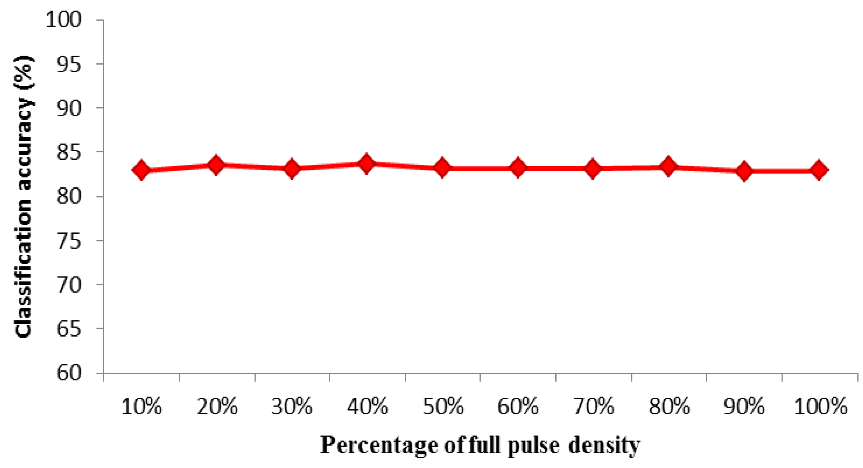
3.2. Effect of Simulated ALS Pulse Density

ALS metrics h10, Hstd and p70 were also used in analyzing the effect of pulse density in classification of Scots pine defoliation. Simulated approximate pulse densities varied between 2 and 20 pulses/m2 with 10% intervals. ALS metrics were calculated and classifications done for 10 different pulse densities for classification scheme DEF1. RF classification did not appear to be particularly sensitive to pulse density. The mean overall classification accuracies varied between 82.8% and 83.7% with respective mean kappa-values of 0.62 and 0.64 (Standard deviations of 1.3% and 1.4%) (Table 6 and Figure 3).
Table 6. The overall classification accuracies (CA), minimum and maximum accuracies, standard deviation, and kappa-values for different pulse densities.
% of full pulse densityPulse density (appr.)CA (%)Kappa-ValueCAmin (%)CAmax (%)CAstd (%)
10%2082.90.6380.584.71.4
20%1883.50.6480.684.91.1
30%1683.10.6381.185.00.9
40%1483.70.6482.884.71.4
50%1283.20.6380.785.21.5
60%1083.20.6381.585.71.4
70%883.10.6381.584.80.6
80%683.30.6481.584.71.3
90%482.80.6281.684.61.3
100%282.90.6381.184.81.5
Figure 3. Overall classification accuracy for defoliation with different ALS pulse densities.
Forests 04 00386 g003

4. Discussion

Forest inventory, mapping and monitoring methods have rapidly developed in recent decades. New methods are more often based on RS applications, especially using ALS. While the methods are changing and forest disturbances are becoming more abundant, there is an urgent need for new methods to map and monitor forest health. In the present study, statistical ALS metrics were tested in the classification of individual tree defoliation. The RF method with three selected ALS metrics was applied to estimate the accuracy of different combinations of defoliation categories and varying pulse densities.
A total of 701 trees were allocated in five different needle loss category classification combinations having 2–4 defoliation classes. The hypothesis was that a larger portion of ALS hits would penetrate deeper into tree crowns and the statistical ALS metrics differ between healthy and defoliated trees. The RF method showed some promising results using 2–3 defoliation classes, while use of further classes resulted in predictions that were only moderately accurate. However, RF was able to classify most of the trees in every classification scheme at least to the adjacent defoliation class. By analyzing classification accuracy of ALS data that was randomly thinned into 10 different pulse densities (2–20 pulses/m2), we found that RF classification was not overly sensitive to varying pulse density and that the overall classification accuracies did not vary considerably between different pulse densities.
In several studies, ALS data has been used in the estimation of forest characteristics other than defoliation at both stand- and tree-level (e.g., [30,57,66,67]). The utilization of ALS has been less studied in the field of forest disturbances. For example, Vehmas et al. [68] detected deadwood through canopy gaps, using ALS data [37]. Solberg et al. [42] compared leaf area index (LAI) with ALS data in defoliated Scots pine stands. Kantola et al. [39] tested ALS data combined with aerial imagery for defoliation estimation by RF with two defoliation classes, and obtained an overall classification accuracy of 88.1% (kappa value 0.76). For comparison, Kantola et al. [39] also tested defoliation detection accuracy using only the ALS metrics (classification accuracy 80.7%). Their results with spectral features were slightly better than in the present study, but they used only two distinct defoliation categories, i.e., healthy and heavily defoliated trees. In the present study, all the trees in addition to those having a threshold value were used in the analysis. In addition, the results were also fairly accurate with more than two classes. Vastaranta et al. [48] studied plot-level needle loss prediction for the same study area. They obtained an overall classification accuracy of 84.3% for two classes.
The defoliation level in the field was visually estimated, using the same procedure as the NFI of Finland [23]. However, visual interpretation could easily have caused deviation in the results if the surveyors were not professionals. Naked-eye calibration is essential when two or more researchers are estimating the critical variable. Observers should also be able to distinguish a between years and within year natural variation in foliage biomass. In addition, prevailing conditions could have also caused bias in the defoliation assessment, such as weather, brightness, heavy wind, high tree density, and difficult terrain. Visual needle loss assessment was done with 10% accuracy and there are uncertainties in assessment. Due to these uncertainties, using narrower class limits is not justified.
Most of the trees were classified from ALS data into the correct or adjacent defoliation class. Misclassifications may have originated from the sensitivity of the reference visual defoliation estimation to errors. For example, a tree having an approximately a defoliation level of 20% could have been visually classified into classes of 10% or 30%. Development of better methods for needle loss estimation in the field may also improve the detection rate from ALS data.
All data were collected from trees in the same study area. A typical feature of the study area was that the taller and older trees in the dominant canopy strata were more heavily defoliated than the shorter and younger trees. This pattern is typical of D. pini outbreak dynamics. Ovipositing females prefer the uppermost parts of the crowns, due to higher carbohydrate synthesis in these needles than found under more shaded conditions [20,69]. The high carbohydrate content, particularly of soluble sugars, promotes the survival of the following sawfly generation. D. pini attacks suppressed understory pines only after completely consuming needles of taller trees. To avoid classifying tree height instead of defoliation, pure height features, such as Hmean and Hmax were not used in classification.
The result of the first RF run with all 26 ALS metrics indicated that the mean return intensity could be a powerful predictor of defoliation. In theory, intensity based upon wavelength of 1064 nm in near-infrared area, should differ between healthy and defoliated trees. In practice, the use of intensity is often problematic, because it has to be calibrated. In this study, the intensity was not calibrated. However, the power of raw intensity was also tested. When penetration (pene) was used together with intensity (int) inl classification, overall accuracies of 81.74% and 83.59% were obtained for two classes (DEF1 and DEF2). Based on this result, it could be assumed that a full waveform ALS could allow more accurate classification of defoliation.
The distribution of defoliation levels among trees was uneven in the study area. The number of trees suffering from heavy defoliation was quite limited, due to low daily temperatures in summer 2008. The classification accuracies were higher in healthier tree classes, which may have resulted from the scarcity of heavily defoliated trees. A larger proportion of trees having severe needle loss could improve the classification accuracy.
Recent studies have shown that the distributions of ALS features vary among different site types [70]. In the present study, the site types were not taken into account because they varied only slightly within the study area. The distribution of ALS metrics probably varies depending on the size and hierarchy level of the trees. For example, Korpela et al. [30] found that dominant Scots pines had approximately 5% higher mean return intensity than the intermediate trees. In the present study, the smaller trees from the suppressed canopy cover level were excluded, but there is still considerable variability in the data.
Results of this study suggest that it may be possible to detect trees with differing levels of needle loss, although the detection accuracy showed less success with increasing numbers of defoliation classes. The results of the present study can be useful for improving the use of ALS in detection and mapping of damage by defoliating insects, which is usually a rare and clustered phenomenon. This study may also support further development of methodologies for inventorying defoliating pests. For example, with remote sensing data, the stratification could be carried out by focusing on areas where pest damage could be detected from preliminary remote sensing data. Suitable class intervals could be set at reasonable threshold levels to obtain adequate estimates, depending upon the nature of the forest disturbance in question.
To the best of our knowledge, the use of ALS-based ITD inventory for estimating tree defoliation has not been widely investigated. However, the results of this study are in some ways comparable with other studies using RS data in needle loss estimation. Ilvesniemi [71] used the same Palokangas study area that was utilized here when investigating the use of aerial photographs and Landsat Thematic Mapper (TM) data in classifying defoliation of Scots pine at the plot level. The classification accuracies for features extracted from aerial photographs varied between 38% (nine classes) and 87.3% (two classes). The best explanatory variable for needle loss was maximum radiation of the near-infrared (NIR) channel in aerial images (r2 = 0.69). Classification results with Landsat image features were slightly poorer (accuracies between 25.4% and 88.7%). Aerial images have also been utilized in other studies to detect tree-wise defoliation such as by Haara and Nevalainen [72]. Their results showed that the tree-wise classification accuracy for reference data of Norway spruce (Picea abies (L.) Karsten) was 68.9% with four classes.
Karjalainen et al. [73] used multitemporal European Remote-Sensing Satellite 2 (ERS-2) and Environmental Satellite (Envisat) satellite images and calculated the synthetic aperture radar (SAR) backscattering intensities (squared amplitude) of 400-m × 400-m grid cells. These SAR features were used to estimate defoliation (same two classes as used here). An overall classification accuracy of 67.8% was obtained, when 30% of the field reference was used in training and 70% for testing the model.
Vastaranta et al. [48] also studied the effect of pulse density for mapping plot-wise defoliation and their results were similar to this study. No remarkable sensitivity for pulse density was found in prediction. According to Kaartinen et al. [66] the pulse density may not affect the individual tree detection. In this study, the tree identification was only done with full pulse density data (~20 pulses/m2).
The present study is one of the first steps towards developing an ALS-based system for monitoring changes in forest health (defoliation) in Finland. Optimally, defoliation mapping should be adopted in current annual practices. For example, it should be part of NFIs or operational forest management planning based on ALS inventory. Field surveys could provide information for growing stock estimation, precise information on defoliating pest agents and also coarse data on needle defoliation. Then, ALS data can be applied on demand to create maps for stem volume and defoliation status where precise information is needed.
Further studies are planned to focus on more heterogeneous forest stands with variable terrain and tree species combinations that represent more extensively forests in Finland than our rather homogeneous test site. The distribution of ALS metrics among different fertility classes also needs investigation. From a practical point of view, it is most critical to detect areas of severe defoliation and test the method with all possible forest site combinations represented. However, it is difficult to predict where and when the mass outbreaks of defoliators will appear. The optimal ALS metric selection method to use in estimating and mapping needle loss also requires further study.

5. Conclusions

In this study the distributions of statistical ALS metrics of healthy and defoliated Scots pines were investigated and levels of defoliation for different defoliation category classification schemes were classified. In addition, 10 varying ALS pulse densities were simulated to investigate if the classification method was sensitive to varying ALS pulse densities. The distributions of ALS statistical metrics varied between healthy and defoliated trees and up to 86.5% (kappa value 0.57) overall classification accuracy for two defoliation classes of Scots pine was achieved using ALS metrics of 10th height percentile, proportion of canopy returns below 80% of relative height and standard deviation of heights as explanatory variables. The classification accuracy decreased with the number of additional defoliation classes, although the method was not overly sensitive to ALS pulse density. However, further studies are needed on more heterogeneous sites to further develop methods for annual disturbance monitoring and mapping, and operational forest management planning.

Acknowledgments

This study was made possible by financial aid from the Maj and Tor Nessling Foundation, Foresters Foundation, Niemi Foundation, Graduate School in Forest Sciences and the Academy of Finland (project Improving Forest Supply Chain by Means of Advanced Laser Measurements (L-IMPACT)). We also wish to thank Tornator Ltd. for fruitful cooperation, James L. Tracy for proofreading and Texas A & M University, Knowledge Engineering Laboratory (KEL) for providing excellent facilities.

Conflicts of Interest

The authors declare no conflict of interest.

References

  1. Attiwill, P.M. The disturbances of forest ecosystems: The ecological basis for conservative management. For. Ecol. Manag. 1994, 63, 247–300. [Google Scholar] [CrossRef]
  2. Linke, J.; Betts, M.G.; Lavigne, M.B.; Franklin, S.E. Introduction: Structure, Function, and Change of Forest Landscapes. In Understanding Forest Disturbance and Spatial Pattern; Wulder, M.A., Franklin, S.E., Eds.; CRC Press, Taylor & Francis Group: Boca Raton, FL, USA, 2007; pp. 1–29. [Google Scholar]
  3. Dale, V.H.; Joyce, L.A.; McNulty, S.; Neilson, R.P.; Ayres, M.P.; Flannican, M.D.; Hanson, P.J.; Irland, L.C.; Lugo, A.E.; Peterson, C.J.; et al. Climate change and forest disturbances. Bioscience 2001, 51, 723–734. [Google Scholar] [CrossRef]
  4. Fleming, R.A.; Candau, J.; McAlpine, R. Landscape scale analysis of interactions between insect defoliation and forest fire in central Canada. Clim. Chang 2002, 55, 251–272. [Google Scholar] [CrossRef]
  5. Lyytikäinen-Saarenmaa, P.; Tomppo, E. Impact of sawfly defoliation on growth of Scots pine Pinus sylvestris (Pinaceae) and associated economic losses. Bull. Entomol. Res. 2002, 92, 137–140. [Google Scholar]
  6. Lyytikäinen-Saarenmaa, P.; Niemelä, P.; Annila, E. Growth Responses and Mortality of Scots Pine (Pinus sylvestris L.) after a Pine Sawfly Outbreak. In Proceedings of Forest Insect Population Dynamics and Host Influences, International Symposium of IUFRO, Kanazawa, Japan, 14–19 September 2003; Liebhold, A.L., Quiring, D.T., Clancy, K.M., Eds.; 2006; pp. 81–85. [Google Scholar]
  7. IPCC, Summary for Policymakers. In Climate Change 2007: The Physical Science basis; Solomon, S.; Qin, D.; Manning, M.; Chen, Z.; Marquis, M.; Avyret, K.B.; Tignor, M.; Miller, H.L. (Eds.) Cambridge University Press: Cambridge, UK, 2007.
  8. Netherer, S.; Schopf, A. Potential effects of climate change on insect herbivores in European forests—General aspects and the pine processionary moth as specific example. For. Ecol. Manag. 2010, 259, 831–838. [Google Scholar] [CrossRef]
  9. Seidl, R.; Schelaas, M.; Lexar, M. Unraveling the drivers of intensifying forest disturbance regimes in Europe. Glob. Chang Biol. 2011, 17, 2842–2852. [Google Scholar] [CrossRef]
  10. Volney, W.J.A.; Fleming, R.A. Climate change and impacts of boreal forest insects. Agr. Ecosyst. Environ. 2000, 82, 283–294. [Google Scholar] [CrossRef]
  11. Walther, G.R.; Post, E.; Convey, P.; Menzel, A.; Parmesan, C.; Beebee, T.J.C.; Fromentin, J.-M.; Hoegh-Guldberg, O.; Bairlein, F. Ecological responses to recent climate change. Nature 2002, 416, 389–395. [Google Scholar]
  12. Björkman, C.; Bylund, H.; Klapwijk, M.J.; Kollberg, I.; Schroeder, M. Insect pests in future forests: More severe problems? Forests 2011, 2, 474–485. [Google Scholar] [CrossRef]
  13. Bale, J.S.; Masters, G.J.; Hodkinson, I.D.; Awmack, C.; Bezemer, T.M.; Brown, V.K.; Butterfield, J.; Buse, A.; Coulson, J.C.; Farrar, J.; et al. Herbivory in global climate change research: Direct effects of rising temperatures on insect herbivores. Glob. Chang Biol. 2002, 8, 1–16. [Google Scholar] [CrossRef]
  14. Logan, J.A.; Regniere, J.; Powell, J.A. Assessing the impacts of global warming on forest pest dynamics. Front. Ecol. Environ. 2003, 1, 130–137. [Google Scholar] [CrossRef]
  15. Régniére, J. Predicting insect continental distributions from species physiology. Unasylva 2009, 60, 37–42. [Google Scholar]
  16. Lindner, M.; Maroschek, M.; Netherer, S.; Kremer, A.; Barbati, A.; Garcia-Gonzalo, J.; Seidl, R.; Delzon, S.; Corona, P.; Kolström, M.; et al. Climate change impacts, adaptive capacity, and vulnerability of European forest ecosystems. For. Ecol. Manag. 2010, 259, 698–709. [Google Scholar] [CrossRef]
  17. Battisti, A.; Stastny, M.; Buffo, E.; Larsson, S. A rapid altitudinal range expansion in the pine processionary moth produced by the 2003 climatic anomaly. Glob. Chang Biol. 2006, 12, 662–671. [Google Scholar]
  18. Vanhanen, H.; Veteli, T.O.; Päivinen, S.; Kellomäki, S.; Niemelä, P. Climate change and range shifts in two insect defoliators: Gypsy moth and nun moth—A model study. Silva Fenn. 2007, 41, 621–638. [Google Scholar]
  19. Hlásny, T.; Zajičková,, L.; Turčáni, M.; Holuša, J.; Sitková, Z. Gepgraphical variability of Spruce bark beetle development under climate change in the Czech Republic. J. For. Sci. 2011, 57, 242–249. [Google Scholar]
  20. De Somviele, B.; Lyytikäinen-Saarenmaa, P.; Niemelä, P. Stand edge effects on distribution and condition of Diprionid sawflies. Agr. For. Entomol. 2007, 9, 17–30. [Google Scholar]
  21. Lyytikäinen-Saarenmaa, P.; Holopainen, M.; Ilvesniemi, S.; Haapanen, R. Detecting pine sawfly defoliation by means of remote sensing and GIS. Forstsch. Aktuell. 2008, 44, 14–15. [Google Scholar]
  22. Juutinen, P.; Varama, M. Ruskean mäntypistiäisen (Neodiprion sertifer) esiintyminen Suomessa vuosina 1966–83. Folia For. 1986, 662, 1–39. [Google Scholar]
  23. Tomppo, E. The Finnish National Forest Inventory. In Forest Inventory; Kangas, A., Maltamo, M., Eds.; Springer: Dordrecht, The Netherlands, 2006; pp. 179–194. [Google Scholar]
  24. Hall, R.J.; Skakun, R.S.; Arsenault, E.J. Remotely Sensed Data in the Mapping of Insect Defoliation. In Understanding Forest Disturbance and Spatial Pattern. Remote Sensing and GIS Approaches; Wulder, M.A., Franklin, S.E., Eds.; CRC Press, Taylor & Francis Group: Boca Raton, FL, USA, 2007; pp. 85–111. [Google Scholar]
  25. Magnussen, S.; Eggermont, P.; LaRiccia, V.N. Recovering tree heights from airborne laser scanner data. For. Sci. 1999, 45, 407–422. [Google Scholar]
  26. Maltamo, M.; Mustonen, K.; Hyyppä, J.; Pitkänen, J.; Yu, X. The accuracy of estimating individual tree variables with airborne laser scanning in boreal nature reserves. Can. J. For. Res. 2004, 34, 1791–1801. [Google Scholar] [CrossRef]
  27. Falkowski, M.J.; Smith, A.M.S.; Hudak, A.T.; Gessler, P.E.; Vierling, L.A.; Crookston, N.L. Automated estimation of individual conifer tree height and crown diameter via two-dimensional spatial wavelet analysis of lidar data. Can. J. Remote Sens. 2006, 32, 153–161. [Google Scholar] [CrossRef]
  28. Bortolot, Z.; Wynne, R.H. Estimating forest biomass using small footprint LiDAR data: An individual tree-based approach that incorporates training data. ISPRS J. Photogramm. Remote Sens. 2005, 59, 342–360. [Google Scholar] [CrossRef]
  29. Van Aardt, J.A.N.; Wynne, R.H.; Scrivani, J.A. Lidar-based mapping of forest volume and biomass by taxonomic group using structurally homogenous segments. Photogramm. Eng. Remote Sens. 2008, 74, 1033–1044. [Google Scholar]
  30. Korpela, I.; Ørka, H.O.; Maltamo, M.; Tokola, T.; Hyyppä, J. Tree species classification using airborne LiDAR—Effects of stand and tree parameters, downsizing of training set, intensity normalization, and sensor type. Silva Fenn. 2010, 44, 319–339. [Google Scholar]
  31. Hyyppä, J.; Kelle, O.; Lehikoinen, M.; Inkinen, M. A segmentation-based method to retrieve stem volume estimates from 3-D tree height models produced by laser scanners. Geosci. Remote Sens. 2001, 39, 969–975. [Google Scholar] [CrossRef]
  32. Wallerman, J.; Holmgren, J. Estimating field-plot data of forest stands using airborne laser scanning and SPOT HRG data. Remote Sens. Environ. 2007, 110, 501–508. [Google Scholar]
  33. Means, J.E.; Acker, S.A.; Fitt, B.J.; Renslow, M.; Emerson, L.; Hendrix, C.J. Predicting forest stand characteristics with airborne scanning ALS. Photogramm. Eng. Remote Sens. 2000, 66, 1367–1371. [Google Scholar]
  34. Næsset, E. Predicting forest stand characteristics with airborne scanning laser using a practical two-stage procedure and field data. Remote Sens. Environ. 2002, 80, 88–99. [Google Scholar] [CrossRef]
  35. Holmgren, J.; Persson, A. Identifying species of individual trees using airborne laser scanner. Remote Sens. Environ. 2004, 90, 415–423. [Google Scholar] [CrossRef]
  36. Brandtberg, T. Classifying individual tree species under leaf-off and leaf-on conditions using airborne lidar. ISPRS J. Photogramm. Remote Sens. 2007, 61, 325–340. [Google Scholar] [CrossRef]
  37. Holopainen, M.; Vastaranta, M.; Rasinmäki, J.; Kalliovirta, J.; Mäkinen, A.; Haapanen, R.; Melkas, T.; Yu, X.; Hyyppä, J. Uncertainty in timber assortment estimates predicted from forest inventory data. Eur. J. For. Res. 2010, 129, 1131–1142. [Google Scholar] [CrossRef]
  38. Vastaranta, M.; Holopainen, M.; Yu, X.; Hyyppä, J.; Hyyppä, H. Predicting stand-thinning maturity from airborne laser scanning data. Scand. J. For. Res. 2010, 26, 187–196. [Google Scholar]
  39. Kantola, T.; Vastaranta, M.; Yu, X.; Lyytikäinen-Saarenmaa, P.; Holopainen, M.; Talvitie, M.; Kaasalainen, S.; Solberg, S.; Hyyppä, J. Classification of defoliated trees using tree-level airborne laser scanning data combined with aerial images. Remote Sens. 2010, 2, 2665–2679. [Google Scholar] [CrossRef]
  40. Vastaranta, M.; Korpela, I.; Uotila, A.; Hovi, A.; Holopainen, M. Mapping of snow-damaged trees in bi-temporal airborne LiDAR data. Eur. J. For. Res. 2012, 131, 1217–1228. [Google Scholar] [CrossRef]
  41. Vastaranta, M.; Holopainen, M.; Yu, X.; Haapanen, R.; Melkas, T.; Hyyppä, J.; Hyyppä, H. Individual tree detection and area-based approach in retrieval of forest inventory characteristics from low-pulse airborne laser scanning data. Photogramm. J. Fin. 2011, 22, 1–13. [Google Scholar]
  42. Sohlberg, S.; Næsset, E.; Hanssen, K.H.; Christiansen, E. Mapping defoliation during a severe insect attack on Scots pine using airborne laser scanning. Remote Sens. Environ. 2006, 102, 364–376. [Google Scholar] [CrossRef]
  43. Hawbaker, T.J.; Keuler, N.S.; Lesak, A.A.; Gobakken, T.; Contrucci, K.; Radeloff, V.C. Improved estimates of forest vegetation structure and biomass with a ALS-optimized sampling design. J. Geophys. Res. Lett. 2009, 114. [Google Scholar] [CrossRef]
  44. Zhao, K.; Popescu, S.; Nelson, R. ALS remote sensing of forest biomass: A scale-invariant estimation approach using airborne lasers. Remote Sens. Environ. 2009, 113, 182–196. [Google Scholar] [CrossRef]
  45. Hanssen, K.; Solberg, S. Assessment of defoliation during a pine sawfly outbreak: Calibration of airborne laser scanning data with hemispherical photography. For. Ecol. Manag. 2007, 250, 9–16. [Google Scholar] [CrossRef]
  46. Solberg, S. Mapping gap fraction, LAI and defoliation using various ALS penetration variables. Int. J. Remote Sens. 2010, 32, 1227–1244. [Google Scholar] [CrossRef]
  47. Räty, M.; Kankare, V.; Yu, X.; Holopainen, M.; Vastaranta, M.; Kantola, T.; Hyyppä, J.; Viitala, R. Tree Biomass Estimation Using ALS Features. In Proceedings of Silvilaser, the 11th International Conference on ALS Applications for Assessing Forest Ecosystems, Hobart, Australia, 16–20 November 2011.
  48. Vastatanta, M.; Kantola, T.; Lyytikäinen-Saarenmaa, P.; Holopainen, M.; Kankare, V.; Wulder, M.; Hyyppä, J.; Hyyppä, H. Area-Based Mapping of Defoliation of Scots Pine Stands Using Airborne Scanning LiDAR. Remote Sens. 2013, 5, 1220–1234. [Google Scholar] [CrossRef]
  49. Hyyppä, J.; Jaakkola, A.; Hyyppä, H.; Kaartinen, H.; Kukko, A.; Holopainen, M.; Zhu, L.; Vastaranta, M.; Kaasalainen, S.; Krooks, A.; et al. Map Updating and Change Detection Using Vehicle-Based Laser Scanning. In Proceedings of JURSE 2009, Shanghai, China, 20–22 May 2009.
  50. Cajander, A.K. The theory of forest types. Acta For. Fenn. 1926, 29, 1–108. [Google Scholar]
  51. Axelsson, P. DEM Generation from Laser Scanner Data Using Adaptive TIN Models. In Proceedings of XIX ISPRS Congress, Commission I–VII, Amsterdam, The Netherlands, 16–23 July 2000; pp. 110–117.
  52. Talvitie, M.; Kantola, T.; Holopainen, M.; Lyytikainen-Saarenmaa, P. Adaptive cluster sampling in inventorying forest damage by the common pine sawfly (Diprion pini). J. For. Plan. 2011, 16, 141–148. [Google Scholar]
  53. Thompson, S.K. Adaptive cluster sampling. J. Am. Stat. Assoc. 1990, 85, 1050–1059. [Google Scholar] [CrossRef]
  54. Roesch, F.A., Jr. Adaptive cluster sampling for forest inventories. For. Sci. 1993, 39, 655–669. [Google Scholar]
  55. Eichhorn, J. Manual on Methods and Criteria for Harmonized Sampling, Assessment, Monitoring and Analysis of the Effects of Air Pollution on Forests. Part II. Visual Assessment of Crown Condition and Submanual on Visual Assessment of Crown Condition on Intensive Monitoring Plots; United Nations Economic Commission for Europe Convention on Long-Range Transboundary Air Pollution: Hamburg, Germany, 1998. [Google Scholar]
  56. Hyyppä, J.; Inkinen, M. Detecting and estimating attributes for single trees using laser scanner. Photogramm. J. Fin. 1999, 16, 27–42. [Google Scholar]
  57. Yu, X.; Hyyppä, J.; Holopainen, M.; Vastaranta, M.; Viitala, R. Predicting individual tree attributes from airborne laser point clouds based on random forest technique. ISPRS J. Photogramm. Remote Sens. 2011, 66, 28–37. [Google Scholar] [CrossRef]
  58. Breiman, L. Random forests. Mach. Learn. 2001, 45, 5–32. [Google Scholar] [CrossRef]
  59. Crookston, N.L.; Finley, A.O. yaImpute: AR package for e_cient nearest neighbor imputation routines, variance estimation, and mapping. Available online: http://cran.r-project.org (accessed on 10 November 2012).
  60. Falkowski, M.; Hudak, A.; Crookston, N.; Gessler, P.; Smith, A. Landscape-scale parameterization of a tree-level forest growth model: A k-NN imputation approach incorporating LiDAR data. Can. J. For. Res. 2010, 40, 184–199. [Google Scholar] [CrossRef]
  61. Hudak, A.; Crookston, N.; Evans, J.; Hall, D.; Falkowski, M. Nearest neighbor imputation of species-level, plot-scale forest structure attributes from LiDAR data. Remote Sens. Environ. 2008, 112, 2232–2245. [Google Scholar]
  62. Latifi, H.; Nothdurft, A.; Koch, B. Non-parametric prediction and mapping of standing timber volume and biomass in temperate forest: Application of multiple optical/ALS-derived predictors. Forestry 2010, 83, 395–407. [Google Scholar] [CrossRef]
  63. Falkowski, M.J.; Evans, J.S.; Martinuzzi, S.; Gessler, P.E.; Hudak, A.T. Characterizing forest succession with ALS data: An evaluation for the Inland Northwest, USA. Remote Sens. Environ. 2009, 113, 946–956. [Google Scholar] [CrossRef]
  64. Kaartinen, H.; Hyyppä, J. EuroSDR/ISPRS Project Commission II, Tree Extraction, Final Report; EuroSDR, 2008. Available online: http://bono.hostireland.com/~eurosdr/publications/53.pdf (accessed on 10 November 2012).
  65. Kaartinen, H.; Hyyppä, J.; Yu, X.; Vastaranta, M.; Hyyppä, H.; Kukko, A.; Holopainen, M.; Heipke, C.; Hirschmugl, M.; Morsdorf, F.; et al. An international comparison of individual tree detection and extraction using airborne laser scanning. Remote Sens. 2012, 4, 950–974. [Google Scholar] [CrossRef] [Green Version]
  66. Vauhkonen, J.; Korpela, I.; Maltamo, M.; Tokola, T. Imputation of single-tree attributes using airborne laser scanning-based height, intensity and alpha shape metrics. Remote Sens. Environ. 2010, 114, 1263–1276. [Google Scholar] [CrossRef]
  67. Vastaranta, M.; Korpela, I.; Uotila, M.; Hovi, A.; Holopainen, M. Area-Based Snow Damage Classification of Forest Canopies Using Bi-Temporal Lidar Data. In Proceedings of ISPRS Workshop on Laser Scanning 2011, Calgary, AB, Canada, 29–31 August 2011; p. 5.
  68. Vehmas, M.; Packalén, P.; Maltamo, M. Assessing Deadwood Existence in Canopy Gaps by Using ALS Data. In Proceedings of Silvilaser 2009, College Station, TX, USA, 14–16 October 2009.
  69. Lyytikäinen, P. Effects of natural and artificial defoliations on sawfly performance and foliar chemistry of Scots pine saplings. Ann. Zool. Fenn. 1994, 31, 307–318. [Google Scholar]
  70. Vehmas, M.; Eerikäinen, K.; Peuhkurinen, J.; Packalén, P.; Maltamo, M. Airborne laser scanning for the site type identification of mature boreal forest stands. Remote Sens. 2011, 3, 100–116. [Google Scholar] [CrossRef]
  71. Ilvesniemi, S. Numeeriset Ilmakuvat ja Landsat TM-Satelliittikuvat Männyn Neulaskadon Arvioinnissa (in Finnish); Helsingin yliopisto: Helsinki, Finland, 2009; p. 62. [Google Scholar]
  72. Haara, A.; Nevalainen, S. Detection of dead or defoliated spruces using digital aerial data. For. Ecol. Manag. 2002, 160, 97–107. [Google Scholar] [CrossRef]
  73. Karjalainen, M.; Kaasalainen, S.; Hyyppä, J.; Holopainen, M.; Lyytikäinen-Saarenmaa, P.; Krooks, A.; Jaakkola, A. SAR Satellite Images and Terrestrial Laser Scanning in Forest Damages Mapping in Finland. In Proceedings of ESA Living Planet Symposium 2010 ESA Special Publication, Bergen, Norway, 28 June–2 July 2010.

