Article

DAYCENT Simulations to Test the Influence of Fire Regime and Fire Suppression on Trace Gas Fluxes and Nitrogen Biogeochemistry of Colorado Forests

Graduate Degree Program in Ecology, Colorado State University, Fort Collins, CO 80523, USA
*
Author to whom correspondence should be addressed.
Current address: Department of Science and Mathematics, Cedarville University, 251 N Main Street, Cedarville, OH 45314, USA.
Current address: Department of Botany, Department of Ecosystem Science and Management, Program in Ecology, and Environment and Natural Resources Program, University of Wyoming, Laramie, WY 82072, USA.
Forests 2012, 3(3), 506-527; https://doi.org/10.3390/f3030506
Submission received: 3 May 2012 / Revised: 6 June 2012 / Accepted: 9 July 2012 / Published: 24 July 2012
(This article belongs to the Special Issue Long-Term Effects of Fire on Forest Soils)

Abstract

:
Biological activity and the physical environment regulate greenhouse gas fluxes (CH4, N2O and NO) from upland soils. Wildfires are known to alter these factors such that we collected daily weather records, fire return intervals, or specific fire years, and soil data of four specific sites along the Colorado Front Range. These data were used as primary inputs into DAYCENT. In this paper we test the ability of DAYCENT to simulate four forested sites in this area and to address two objectives: (1) to evaluate the short-term influence of fire on trace gas fluxes from burned landscapes; and (2) to compare trace gas fluxes among locations and between pre-/post- fire suppression. The model simulations indicate that CH4 oxidation is relatively unaffected by wildfire. In contrast, gross nitrification rates were reduced by 13.5–37.1% during the fire suppression period. At two of the sites, we calculated increases in gross nitrification rates (>100%), and N2O and NO fluxes during the year of fire relative to the year before a fire. Simulated fire suppression exhibited decreased gross nitrification rates presumably as nitrogen is immobilized. This finding concurs with other studies that highlight the importance of forest fires to maintain soil nitrogen availability.

1. Introduction

Fire regimes are determined by the interaction of climate, fuels/plant community, and ignitions [1,2]. Regional to local climate dictates biomass accumulation and fuel ignitions, which taken together, determine a location’s fire regime [1]. A moist climate may allow for greater fuel accumulation while simultaneously making that fuel less likely to be ignited, whereas the opposite would be expected to occur in a dry climate: lower fuel accumulation, but more easily ignited. The interplay among these three factors is of great interest as scientists continue to try and discern the importance of human influence on western U.S. forests and their fire regimes [3].
In the western U.S., we have the most extensive and detailed fire history records in the world [4]. However, knowledge of fire activity does not always translate into an understanding of forest structure and function for those same periods of time. In particular, there is great interest and concern regarding the consequences of fire suppression and exclusion (which includes grazing effects) over the past century [5] on ecosystem structure and function, relative to the natural range of variability.
Despite its importance, relatively little research has related biomass accumulation and Colorado Front Range fire regimes. Warmer and drier conditions in the American West [6] have increased wildfire frequency and extent over the past three decades [7]. Global circulation models (GCMs) predict that these conditions will continue as greenhouse gases continue to accumulate in the atmosphere [6]. We are interested in understanding the extent to which natural variability and fire suppression practices on the source-sink strength of greenhouse gases, and how important the two-way interaction may be between fire and climate [8].
Ecosystem modeling is particularly valuable for evaluating the sensitivity of ecosystem structure and functions to natural variability and management (such as fire suppression), especially for dynamic and highly variable processes that are difficult to estimate in the field, such as trace gas fluxes. Simulation models allow one to extrapolate across spatial variability and through time, and to evaluate historical situations that no longer occur. Our objectives in this study are to examine the DAYCENT model’s ability to simulate [9,10,11] a ponderosa pine forest, and then:
  • Evaluate the short-term impact of fire on trace gas fluxes and N biogeochemistry from burned landscapes.
  • Examine trace gas fluxes and N biogeochemistry in response to hypothetical fire regimes among locations and pre-/post- fire suppression.

2. Experimental Section

2.1. Model Description

The DAYCENT model [10] is the daily time step version of the CENTURY model [12,13]. Both models simulate the flow of carbon (C), nitrogen (N), phosphorus (P), and sulfur (S), as they cycle with production and decomposition of organic matter (plant and soil) through a simulated ecosystem. The DAYCENT 4.5 model includes daily representations of soil moisture, temperature, and N availability. Required model inputs include daily precipitation (cm) and maximum/minimum daily temperatures (°C), soil depth (divided into 10 layers), and soil characteristics (texture and bulk density). The high temporal resolution of the trace gas submodel allows for daily output of trace gas fluxes (nitrous oxide, nitric oxide, and methane). This improves estimates of gas fluxes, which are greatly variable and dependent upon rapid changes in the soil environment driven by weather variability and biotic processes.
The DAYCENT submodels include plant production, decomposition, methane oxidation, nitrification, and denitrification. The plant production subroutines simulate production, nutrient allocation, and death. These processes are regulated by soil water content, temperature and nutrient availability. Dead and decomposing material enters the soil organic matter (SOM) pools (active, slow, and passive) that are also regulated by the factors that affect production.
The N-gas submodel [11] utilizes the “hole-in-the-pipe” model [14] to represent denitrification (NH4+ to NO3) and nitrification (NO3 to N2) processes. N2O and NO are intermediate molecules for both processes, and each is lost during metabolism to the environment. The rate of these gas losses is dependent upon environmental factors that the N-gas submodel accounts for, including soil water status, temperature, NH4+ and NO3 availability, and respiration rates, to drive calculations of daily N2O and NOx emission rates. The denitrification and nitrification submodels are driven by soil water status, temperature, pH, NH4+ and NO3 availability, labile C availability, O2, soil diffusivity, and respiration rates. No denitrification occurs within the model if the % water-filled-pore-space (% WFPS) falls below 55%. Denitrification rates increase exponentially between 55 and 90% WFPS. Nitrification rates are constrained by the size of the soil NH4+ pool, soil temperature, % WFPS, and pH. Nitrous oxide production is considered to be a constant proportion of the nitrification rate (g N m−2 d−1). Nitrous oxide (NOx) production is directly proportional to N2O production, but also regulated by soil gas diffusivity and % WFPS.
Upland soils are generally found to be sinks for atmospheric CH4 [15]. Del Grosso et al. [9] created a submodel within DAYCENT to simulate this biological process based upon field data collected in a variety of ecosystems, including grasslands, agricultural land, and forests. Methane oxidation is calculated within this submodel based upon soil water status (field capacity), soil texture, and soil bulk density. Each of these factors influence soil gas diffusivity, however, as this becomes less limiting the importance of soil temperature increases.

2.2. Study Sites

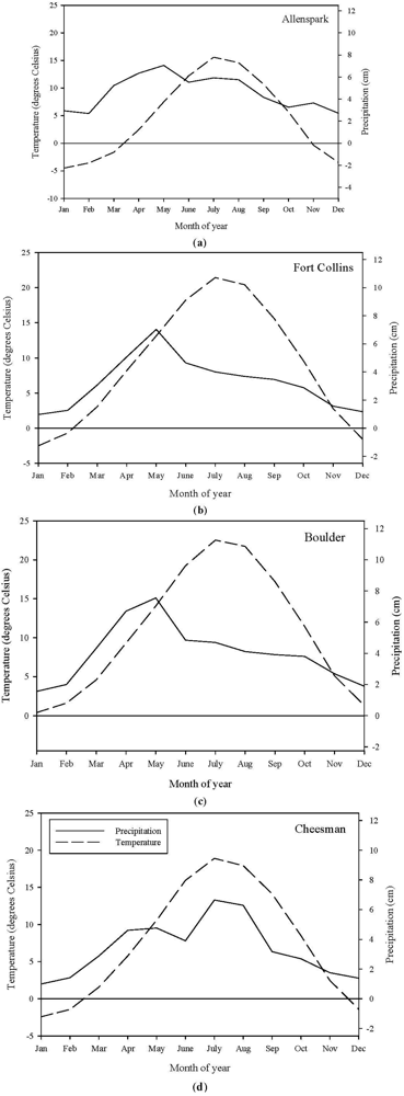
2.2.1. Fire History and Climate Data

We selected four sites to evaluate the response to fire events and fire exclusion practices, both of which are common in the region [16]: Boulder, Allenspark, Cheesman, and Fort Collins, with the intention of capturing a large range of variability in the Front Range of Colorado and maximizing the realm of inference. Each site had complete weather records, fire history documentation in the scientific literature, and field observations of trace gas flux rates.
Weather data were readily available and complete for each location. At three sites [17], the daily weather records exceeded 100 years with the fourth site (Allenspark) having 58 years of record (Table 1). The long period of observation provided a wide spectrum of variability in weather and climate. The climate of the northern Front Range is dry, with the lowest precipitation occurring in the winter. Precipitation is unimodal (Fort Collins and Boulder) to weakly bimodal (Allenspark and Cheesman) with peaks in the late spring (April and May) and/or summer (July and August) (Figure 1). Even during times of increased moisture vegetation can remain stressed due to the greater temperatures that occur concurrently. Mean annual temperature ranges between 4.7 and 11.0 °C at the four sites (Table 1) while mean annual precipitation ranges from 384–520 mm (Table 1).
Table 1. Weather stations with daily weather data to be used in the DAYCENT model [17].
Location
BoulderCheesmanAllensparkFort Collins
Station nameBoulderCheesman ReservoirAllensparkFort Collins
Station ID50,84851,52850,18353,00553,005
CountyBoulderJeffersonBoulderLarimerLarimer
Years of record1898–20061903–20061948–19931994–20061900–2006
Data years1081034513106
Latitude (°N)40° 0'39° 13'40° 12' 40° 37'
Longitude (°W)105° 16'105° 17'105° 32' 105° 08'
Elevation (m)1,6712,0972,606 1,525
MAP (cm)48.641.252.8 38.4
MAT (°C)117.24.7 8.9
Figure 1. Monthly precipitation (cm, solid line) and mean temperatures (°C, dashed line) for Fort Collins (b); Boulder (c); Allenspark (a); and Cheesman (d) weather stations.
Forests 03 00506 g001
At each of these four sites we found estimates for fire return intervals (Table 2). Brown et al. [3] found that composite fire return intervals generally ranged between 6 and 12 years for Cheesman, though there were long periods (1723–2000, with fires in years 1723 and 1851) where fires were much less frequent. Two of the sites, Boulder and Allenspark, are located in Boulder County, Colorado where Veblen et al. [18] conducted an extensive fire history study. Boulder had an average fire return interval of 14 years with exact fire scar dates back to 1679. Sites near Allenspark had an average fire return interval of 40 years based on fire scar chronologies that date back to 1541. For the DAYCENT modeling we constrained the number of fires at these sites by selecting only the fire years during which at least 10% of the examined trees had recorded a fire scar. In order to make a good estimate of fire return interval for the Fort Collins site, we interpolated the fire return interval from an equation developed by Brown and Shepperd [19] for the region that relates fire return interval with latitude. We then pooled that with information from Rocky Mountain National Park [20]. These patterns of fire return interval are dictated in large part by the climate of the region and the individual sites that vary both in latitude and altitude.
Table 2. Time period(s) modeled using DAYCENT, including fire return intervals (years) or fire dates (year A.D.) for a particular time period at a specific site. Fire record data for each of these sites were retrieved from the literature source cited. These data were coded into the DAYCENT schedule file (*.sch) to reflect the same event chronology as that site had experienced in the past.
LocationModeled PeriodFire Return Interval (Years) or Fire Date (Year)Source
Cheesman1–12859Brown et al. [3]
1286–150012
1501–16006
1601–171510
1715–20001723, 1851 (no further fires)
Boulder1–165014Veblen et al. [18]
1651–19201679,1691,1703,1708,1713,1716, 1722, 1725, 1732, 1737, 1747, 1786, 1789,1795, 1813, 1841, 1847, 1851, 1860, 1868, 1870, 1880, 1884, 1886, 1908, 1910Sites 15 (1853–1914 m, >10% of trees scarred)
1921–2000Fire suppression
Allenspark1–150040Veblen et al. [18]
1501–19201541, 1602, 1654, 1745, 1768, 1814, 1859, 1880Sites 18, 19 (2414–2682 m, >10% of trees scarred)
1921–2000Fire suppression
Fort Collins1–19201921–200030Fire suppressionSherrif and Veblen [20] Brown and Shepperd [19]

2.2.2. Study Sites-Vegetation and Soils

A dynamic ecotone is formed as the grasslands of the Great Plains merge into the forests of the foothills of the Colorado Front Range. We focused on two forest types within this ecotone, lower elevation ponderosa pine stands (that tend to be open with substantial grass, 1800–2100 meters) and mid-elevation ponderosa pine (that have some canopy closure, mixed with Douglas fir, 2100–2400 meters) [21,22,23,24].
We used site-specific soil data from the online NRCS Soil Survey. The Northern Front Range and Larimer County, Colorado are dominated by soils with a sandy loam texture. A typical soil profile is 0.90 m thick with bedrock at 1 m depth. Soils of Boulder County, Colorado are gravelly loamy sand with soil depths of approximately 1.5 m. At Allenspark, soils profiles are 1.5 m deep with a cobbly and stony sandy loam soil texture. Soils that surround the Cheesman Reservoir are shallow with weathered bedbrock at 0.75 m depth and the soil texture is gravelly throughout the profile. Using the soil texture triangle we converted texture descriptions from the NRCS Soil Survey to % sand, silt, and clay (Table 3).
Table 3. A description of the site specific soil parameters used for each of the four simulated locations. Data shown include the number and thickness of soil layers, bulk density, and soil texture. Site specific soils data were retrieved from the United States Department of Agriculture—Natural Resource Conservation Service’s Web Soil Survey [25].
Layer thickness (cm)Bulk density (mg cm3)Sand and clay (%)
AllensparkBoulderCheesmanFort CollinsAllensparkBoulderCheesmanFort Collins
0 to 21.51.331.331.250.80, 0.130.74, 0.110.71, 0.210.70, 0.20
2 to 51.51.331.51.250.80, 0.130.74, 0.110.75, 0.150.70, 0.20
5 to 101.51.331.51.350.80, 0.130.74, 0.110.75, 0.150.70, 0.20
10 to 201.51.331.51.350.80, 0.130.74, 0.110.75, 0.150.70, 0.20
20 to 301.51.331.61.50.80, 0.130.74, 0.110.80, 0.100.70, 0.20
30 to 451.51.331.61.50.80, 0.130.74, 0.110.80, 0.100.75, 0.15
45 to 601.51.331.61.70.80, 0.130.74, 0.110.80, 0.100.75, 0.15
60 to 751.51.33-1.70.80, 0.130.74, 0.11-0.75, 0.15
75 to 901.51.33-1.70.80, 0.130.74, 0.11-0.75, 0.15
90 to 1051.51.33--0.80, 0.130.74, 0.11--
105 to 1201.51.33--0.80, 0.130.74, 0.11--
120 to 1501.51.33--0.80, 0.130.74, 0.11--

2.3. Model Parameterization

Input required for running DAYCENT simulations includes daily weather (precipitation and temperature) and soil (texture and number of layers) data. These data are fundamental to the land surface submodel that simulates soil water content and soil temperature for each soil layer. We used the DAYCENT_file100 utility to estimate wilting point, field capacity, and saturated hydraulic conductivity (Ks) based on soil texture data for the sites.
We parameterized the model (CROP.100 and TREE.100 plant production subroutines) to simulate grass and tree production, nutrient allocation, and death in a temperate forest ecosystem [26]. Plant death is regulated by temperature, soil water content, and turnover rates. Dead and decomposing material enters the soil organic matter (SOM) pools. We used fire return intervals (FRI) from the scientific literature (Table 2) as the basis for the scheduling of fire events at each site. FRI and fire severity (and intensity) vary inversely [27]. We expressed this relationship in the model by allowing more severe fires when the time since the last fire was great relative to the mean fire return interval. Conversely, we modeled a low severity fire when the most recent fire was less than the mean fire return interval for the site. In the model, at the time of each fire event, biomass pools are multiplied by the user specified coefficient and that portion is removed from the simulation.

2.3.1. Simulation Procedure

Model simulations were initiated with the site-specific soil and weather data described above. We ran a total of four separate simulations, one per site. We initialized the DAYCENT model as a forest ecosystem with a grass component, and simulated plant production with two subroutines: one for the grass understory (CROP.100), and a second for the tree component (TREE.100). We used literature values for other ponderosa pine forests as estimates for initial conditions (pool sizes) for biomass and soil carbon, and ran simulations for each site for 2000 years. Between year 1 and 1500, we scheduled regular fires that reflected the fire return intervals at each site (Table 2). The length of these simulation runs has been found to bring other modeled ecosystems into equilibrium [28]. We examined total soil organic matter pools at each site to verify steady state that we defined as having less than a 5% change in total soil organic matter from year to year. Each of the four simulated sites met this criterion.
At the time of each fire, DAYCENT ran two subroutines, TREM.100 (Table 4) and FIRE.100 (Table 5). The TREM routine removed biomass from trees (and constituent pools) for either a low or high severity fire [29,30]. The FIRE routine worked in a similar fashion except that rather than removing biomass from tree pools, it removed the grass and litter components at rates that correlated to the fire severity. At year 1500, we began to analyze the simulated fluxes (g m−2·yr−1) of CH4, N2O, and NO as well as gross nitrification rates (g N m−2·yr−1) with the intent of observing how they responded to simulated fire events and more recent (circa 1920) fire suppression practices common to the region [16].
Table 4. A description of DAYCENT input parameters for tree removal (TREM.100) events for two fire severity scenarios: surface (low severity) or canopy (high severity) fire.
Surface FireCanopy FireParameterDefinition
11EVNTYPevent type flag (=0 for cutting event, =1 for fire event)
0.50.99REMF (1)fraction of leaf component removed
0.50.90REMF (2)fraction of live branch component removed
0.20.90REMF (3)fraction of large wood live component removed
0.80.99REMF (4)fraction of fine branch dead component removed
0.40.99REMF (5)fraction of large wood dead component removed
0.30.99FD (1)fraction of fine root component that dies
0.10.99FD (2)fraction of coarse root component that dies
0.50RETF (1,1)fraction of C in killed live leaves that is returned to the system (ash or litter)
0.50.3RETF (1,2)fraction of N in killed live leaves that is returned to the system (ash or litter)
11RETF (1,3)fraction of P in killed live leaves that is returned to the system (ash or litter)
00RETF(1,4)fraction of S in killed live leaves that is returned to the system (ash or litter)
0.50RETF(2,1)fraction of C in killed fine branches that is returned to the system (ash or dead fine branches)
0.50.3RETF (2,2)fraction of N in killed fine branches that is returned to the system (ash or dead fine branches)
11RETF (2,3)fraction of P in killed fine branches that is returned to the system (ash or dead fine branches)
00RETF (2,4)fraction of S in killed fine branches that is returned to the system (ash or dead fine branches)
0.30RETF (3,1)fraction of C in killed large wood that is returned to the system (ash or dead large wood)
0.30.3RETF (3,2)fraction of N in killed large wood that is returned to the system (ash or dead large wood)
11RETF (3,3)fraction of P in killed large wood that is returned to the system (ash or dead large wood)
00RETF (3,4)fraction of S in killed large wood that is returned to the system (ash or dead large wood)
Table 5. A description of DAYCENT input parameters for fire events (FIRE.100) events for either a low fire severity or high severity fire scenario. This subroutine removed mass from litter and grass pools.
Fire SeverityParameterDefinition
LowHigh
0.60.8FLFREMfraction of live shoots removed by a fire event
0.60.8FDFREM(1)fraction of standing dead plant material removed by a fire event
0.20.9FDFREM(2)fraction of surface litter removed by a fire event
0.60.9FDFREM(3)fraction of dead fine branches removed by a fire event
0.40.9FDFREM(4)fraction of dead large wood removed by a fire event
0.10.01FRET(1,1)fraction of C in the burned aboveground material (live shoots, standing dead, and litter) returned to the system following a fire event
0.40.4FRET(1,2)fraction of N in the burned aboveground material (live shoots, standing dead, and litter) returned to the system following a fire event
10.4FRET(1,3)fraction of P in the burned aboveground material (live shoots, standing dead, and litter) returned to the system following a fire event
10.4FRET(1,4)fraction of S in the burned aboveground material (live shoots, standing dead, and litter) returned to the system following a fire event
0.0030.003FRET(2,1)fraction of C in the burned dead fine branch material returned to the system following a fire event
0.20.2FRET(2,2)fraction of N in the burned dead fine branch material returned to the system following a fire event
00.4FRET(2,3)fraction of P in the burned dead fine branch material returned to the system following a fire event
00.4FRET(2,4)fraction of S in the burned dead fine branch material returned to the system following a fire event
0.0030.003FRET(3,1)fraction of C in the burned dead dead large wood material returned to the system following a fire event
0.20.2FRET(3,2)fraction of N in the burned dead dead large wood material returned to the system following a fire event
00.4FRET(3,3)fraction of P in the burned dead dead large wood material returned to the system following a fire event
00.4FRET(3,4)fraction of S in the burned dead dead large wood material returned to the system following a fire event
0.20.2FRTSHadditive effect of burning on root/shoot ratio
1010FNUE(1)effect of fire on increase in maximum C/N ratio of shoots
3030FNUE(2)effect of fire on increase in maximum C/N ratio of roots

2.4. Comparison of Model Output and Statistical Analyses

We used two methods to verify the model output and its ability to simulate biogeochemical processes in these forests. First, we compared the model output of plant production (NPP) and total ecosystem carbon with values in the scientific literature for ponderosa pine ecosystems [31,32,33,34,35,36].Law et al. [35] estimated total carbon stocks to be 10 to 21 kg m−2 in Oregon whereas simulations of our sites yielded estimates between 4 and 12 kg·C·m−2. Mean NPP for the four simulated sites ranged between 56–200 g·C·m−2·yr−1. These values fall within the range (76–236 g·C·m−2·yr−1) of NPP estimates by Law et al. [31] for the ponderosa pine forests of Oregon and carbon accumulation (90–281 g·C·m−2·yr−1) estimated by Hicke et al. [32] for the ponderosa pine forests of the Colorado Front Range.
In addition, we compared short-term, infrequent, trace gas flux measurements at locations near to each of the sites [37] to modeled output. We calculated the mean, minimum, maximum, and % CV for simulated methane oxidation, N2O and NO production, gross nitrification (g·m−2·yr−1), and annual precipitation (cm) for each site. We isolated the years that fires were simulated at each site and collected data for the fire year and the years before and after the fire. From these data, we calculated the means and the standard error of the means for the variables mentioned above (Figure 2) in order to determine the short-term influence of the fire. Following the same procedure, we grouped model output into two categories; pre-fire suppression (1500–1920, with hypothetical fire return intervals) and post-fire suppression (1920–2000, no fires). We evaluated the potential influence of large-scale management by comparing means (± SE) within and among sites.
Figure 2. (a) Methane uptake rates (g·CH4·m−2·yr−1); (b) gross nitrification (g·N·m−2·yr−1) and (c) nitric oxide fluxes (g·NO·m−2·yr−1), for each of the four simulated locations. Points represent the means of methane uptake one year prior to, during the year of, and one year after a fire occurred for each site. Error bars are the standard error of the mean.
Forests 03 00506 g002

3. Results and Discussion

3.1. Simulated and Observed Biogeochemistry of Front Range Forests

DAYCENT simulated consistent CH4 uptake rates as across all four sites. Of the four sites we modeled, means ranged between 0.377 and 0.448 g·CH4·m−2·yr−1, and the CV (%) for CH4 uptake was <15% (Table 5). This correspondence among modeled sites reflects the similarity in the climate and soil texture (sandy loams). The CH4 oxidation submodel is largely controlled by soil water content, which interacts with soil texture, to control gaseous diffusion through the soil profile. Del Grosso et al. [9] calculated that maximum CH4 uptake (~0.438 g·CH4·m−2·yr−1) occurs at 7.5% soil volumetric water for coarse textured soils such as the ones we used in these simulations. Field observations in the region [37] were made at soil moisture levels between 2 and 18% and associated flux rates agreed well with those predicted by the beta function used in the CH4 oxidation submodel.
The simulation output suggests that DAYCENT captured this dependence of CH4 uptake on soil moisture levels; Fort Collins, with intermediate levels of precipitation (Table 5) had the greatest CH4 oxidation. In contrast Cheesman (the driest site), and Allenspark (wetter site) were (on an annual basis) below and above, respectively, the optimum soil moisture levels for CH4 oxidation and thus showed lower rates. In his study of coniferous forest soils in Arizona, Hart [38] measured mean methane uptake rates of between 0.229 and 0.479 mg·C·m−2·h−1. These uptake rates were significantly correlated with soil temperature rather than soil water content. While at a slightly lower elevation, the simulated sites in Colorado receive approximately half the precipitation that occurs at Hart’s study sites. Elsewhere in the Front Range, methane uptake rates were measured in urban/agriculture/native [39], alpine [40] and shortgrass steppe [41,42,43] ecosystems. The simulated rates of methane oxidation, ~0.4 g·m−2·y−1 (Table 6), are intermediate to the rates measured at these sites. Smith et al. [44] reviewed the scientific literature and calculated that the mean methane uptake rate of 0.24 g·m−2·y−1 from “natural/semi-natural”, or non-agricultural soils around the globe.
Nitrous oxide flux rates were also similar among the four modeled sites. However, each site exhibited greater variability than CH4 uptake as CVs were >49% within all sites. Means (g·N·m−2·yr−1) of the DAYCENT simulation results for N2O in decreasing order are Allenspark (0.029) > Cheesman (0.014) > Fort Collins (0.011) = Boulder (0.011). These model estimates are similar to the observations of Kaye et al. (2004), for native grassland and cropped wheat systems in northern Colorado where both had mean N2O fluxes of less than 0.05 g·N·m−2·yr−1. In contrast, the N2O fluxes were found to be an order of magnitude greater from urban and agricultural ecosystems that had received N fertilizer. In the southwestern U.S., others observed N2O flux rates of approximately 0.05 g·m−2·yr−1 [38], 0.01 g·m−2·yr−1 [45], and between 0.05 and 0.20 g·m−2·yr−1 [46].
Nitric oxide fluxes were an order of magnitude greater than the N2O fluxes from all but the Allenspark location. We found the following pattern of decreasing NO fluxes (g·m−2·yr−1): Allenspark (0.198) > Fort Collins (0.152) > Boulder (0.129) = Cheesman (0.129). Coefficients of variation (%) for NO fluxes followed a similar pattern and fell within the same range (43.6–85.9%) as observed for the N2O flux rates. The simulated NO flux estimates fall within the range of field measurements from the western U.S. [47,48]. In an Oregon ponderosa pine forest Stark et al. [47] report NO fluxes of 0.009 g·N·m−2·yr−1 whereas Levine et al. [48] report a flux rate of 0.63 g·N·m−2·yr−1 in California chaparral.
Table 6. Mean, minimum, maximum and CV (%) for CH4 uptake, N2O and NO fluxes, nitrification rates and annual precipitation (cm). Mean, maximum and minimum values for fluxes and nitrification are given as g·m−2·yr−1. These descriptive data are derived from the years 1500–2000.
VariableSiteMeanMinimumMaximumCV (%)
CH4 uptakeFort Collins0.4480.3780.5014.2
Allenspark0.3770.2480.51114.8
Boulder0.4270.3560.4685.2
Cheesman0.3980.3310.4325.2
N2O fluxFort Collins0.0110.0020.04849.3
Allenspark0.0290.0040.09952.4
Boulder0.0110.0030.06682.7
Cheesman0.0140.0040.07778.6
NO fluxFort Collins0.1520.0300.67452.1
Allenspark0.1980.0580.69443.8
Boulder0.1290.0330.67685.9
Cheesman0.1290.0360.63780.0
NitrificationFort Collins0.5580.1062.42249.2
Allenspark0.8610.2052.34837.5
Boulder0.5640.1483.30483.1
Cheesman0.6780.1883.86678.2
PrecipitationFort Collins38.919.472.627.2
Allenspark49.123.287.332.5
Boulder47.122.075.523.7
Cheesman35.433.849.120.0
Nitrification rates, or the rate of conversion from NH4+ to NO3, were greatest for the Allenspark simulation (Table 6). Means of the gross nitrification rates ranged between 0.558 and 0.861 g·m−2·yr−1. The maximum rate of nitrification across all sites and years occurred at the Cheesman site with a value of 3.866. Minimum values of nitrification were generally ¼ of the mean; whereas maxima were 4–5 times the site mean (Table 2). Patterns of variability were identical (in rank order) to those that were observed for NO fluxes (Table 6). Gross nitrification rates measured in ponderosa pine forests of Oregon and New Mexico [47,49] were an order of magnitude greater than those calculated from the DAYCENT simulations.

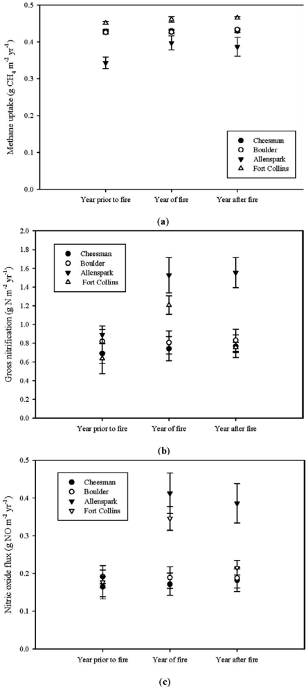
3.2. Effects of Fire on Trace Gas Fluxes

3.2.1. Year Before, of and After Fire

Simulated methane uptake was minimally affected by fire. All four of the sites we modeled exhibited a slightly increasing trend over the three-year period that included the year prior to, the year of, and the year after a fire (Figure 2). Allenspark departed the most from pre-fire years, when methane uptake increased by a mean of 0.05 g·CH4·m−2 during the year of a fire. At one-year post-fire, the mean CH4 uptake had decreased though it was still slightly greater than the mean for one year pre-fire. Allenspark also exhibited the greatest variability of the four sites we modeled. This is best explained by the longer fire return interval (40 years), greater fire severity (high), and climate variability. In contrast, each of the other three sites showed much less variability, suggesting that fire has only a minor effect on CH4 oxidation. None of the factors that control the rate CH4 oxidation in the DAYCENT submodel, field capacity, soil texture and bulk density, are directly impacted by the modeled fire events. If we extrapolate our estimate to incorporate our knowledge of a fire’s burn area we may use these data to estimate the change in sink strength as a result of a single fire event. In 2002 the Hayman fire burned ~55,000 ha around which the Cheesman site was selected. Using these data, we estimate that the net reduction in sink strength between one year before and one-year after that fire would be approximately 55,000 kg CH4 (or 1.0 kg ha−1).
Each of the simulated sites exhibited a large increase in gross nitrification during a fire year relative to the year prior. Simulated N availability following the fires was increased at two of the sites, Fort Collins and Allenspark (Figure 2). This increase persisted into the year after the fire for Allenspark only, with Fort Collins returning to pre-fire levels within a year. Gross nitrification rates were relatively unaffected by fire at both Boulder and Cheesman (Figure 2). We attribute this primarily to the lower severity of the fires (less N lost, Table 4, Table 5) that were simulated at these sites. This is as compared to the Allenspark and Fort Collins sites, which generally had longer fire return intervals and consequentially greater fire severity (greater N lost).
Generally, greater fire severity leads to an increase in gaseous N loss from the forest during the fire. However, this effect of reduced substrate availability decreased as competition for nutrients with plants was also greatly reduced as the high severity fires at Allenspark and Fort Collins removed a large portion of the live vegetation. The model compares well with field data; Hamman et al. [50,51] found that fire severity and altered fire regime can directly influence the soil microbial community structure and biogeochemistry in ponderosa pine forests of the Colorado Front Range. Carreira et al. [52] investigated the effect of a single fire and found that it significantly increased N availability and net nitrification rates. Similar findings have been documented in southwestern U.S. ponderosa pine [53,54] and a variety of other ecosystems [55].
We observed three patterns for gross nitrification means (Figure 2): no change (Boulder), response and return (Cheesman and Fort Collins), and persistent change (Allenspark) over the three-year time period for each fire event. Nitrogenous gas (N2O and NO) fluxes are the result of incomplete oxidation during nitrification or reduction during denitrification. Of the four modeled sites, none had average rainfall greater than 530 mm yr−1. The N-gas submodel is driven by soil moisture and no denitrification occurs when % WFPS < 55% [11]. This was supported by model observation of very low to absent N2 flux, the end product of denitrification [11].
Nitrous and nitric oxide fluxes (Figure 2) followed a nearly identical pattern to simulated gross nitrification rates. Both are by-products of nitrification, and together, they accounted for up to 25% of the gross nitrification N. In a related study [37] we measured in situ N2O fluxes along a chronosequence of fires in the Colorado Front Range. We scaled these data up and calculated a mean flux of 0.002 g N m−2·yr−1. Other sites in the Front Range were estimated to have N2O flux rates between 0.164 and 0.937 g·N·m−2·yr−1. Averaging across all four sites, DAYCENT calculated annual N2O fluxes of 0.016 g·N·m−2·yr−1, which is an order of magnitude above and below these field measurements. These field based studies were limited in their spatial and temporal coverage, whereas DAYCENT appears to have integrated the variability observed in those studies producing an intermediate estimate of N2O fluxes from these systems.

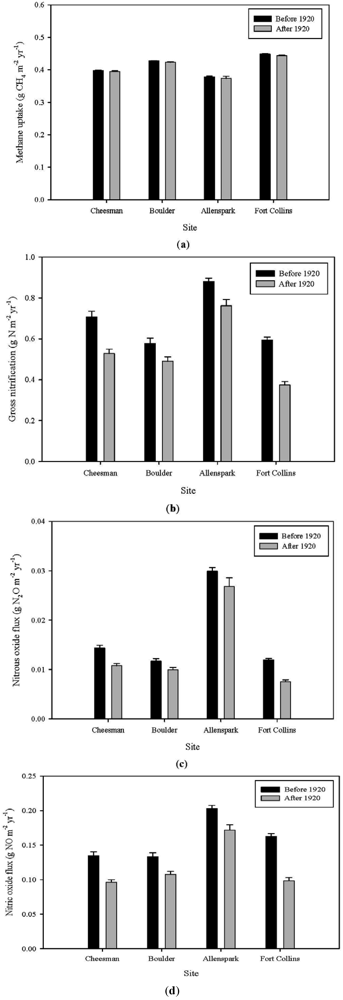
3.2.2. Pre- versus Post-Fire Suppression

Fire suppression practices did not alter methane uptake rates in the DAYCENT simulations (Figure 3). Within site variability was low for these two time periods. We calculate percent difference for pre- and post-fire suppression to be less than 1.2% at all 4 sites. Where methane uptake showed a short term increase immediately following a fire the response appears to be insignificant when considering longer time scales such as a single (hypothetical) fire return interval. While we saw a minor decrease in CH4 uptake, we had expected greater differences to become apparent as fire suppression allowed tree biomass (or tree densities) to increase, which would consequently increase nutrient competition. The simulation data suggest that either methanotrophic bacteria are not in direct competition with plants for nutrients or that the model fails to capture this interaction.
Nitrous oxide fluxes were greatest at Allenspark, which had nearly 3-fold the rates observed at Cheesman, Boulder, and Fort Collins. Based on the model, this outcome is the result of differences in precipitation and soil properties between Allenspark and the other three simulated sites. DAYCENT first partitions N2O fluxes from nitrification and denitrification processes and then sums these values into the single value reported as the N2O flux. At Allenspark, precipitation events stimulated pulses of N2O flux denitrification, whereas similar events at the other three sites were only great enough to stimulate N2O flux from nitrification. Changes in N2O fluxes in response to fire suppression (Figure 3) were greatest at Fort Collins (−36.7%), followed by Cheesman (−25.2%), Boulder (−14.5%), and Allenspark (10.3%). N2O flux rates at these four sites accounted for <1% of gross nitrification. Nitric oxide flux rates (Figure 3) followed the same pattern, although the fluxes were an order of magnitude greater than N2O fluxes. Fire suppression reduced NO fluxes by 39.7% at Fort Collins, 28.6% at Cheesman, 19.0% at Boulder, and 15% at Allenspark. Since the climate wasn’t different during the fire suppression period relative to prior, the changes in N2O and NO flux reflect a change in substrate availability as continued plant uptake during this the fire suppression period led to N immobilization.
We found Allenspark to have the greatest rate of nitrification both before and after fire suppression that was simulated to begin in 1920. Fire suppression decreased gross nitrification rates there the least, by 13.5%, compared to the other three sites: Boulder (−15.2%), Cheesman (−25.3%) and Fort Collins (−37.1%). Stark and Hart [49] measured gross nitrification rates of 25 to 79 mg·N·m−2·d−1 (9.1 g·N·m−2 yr−1 to 28.8 g N·m−2·yr−1) in New Mexican and Oregon ponderosa pine, respectively. Stark and Hart [49] suggest that C and N supplies are the primary controls on gross nitrification rates. They suggest that internal cycling of NO3 is strongly controlled by microbial uptake which can be rapid relative to plant uptake in forested ecosystems. The DAYCENT simulations seem to capture this short-term dynamic as gross nitrification rates increase during the year of the fire (Figure 2). Over longer time scales, the DAYCENT simulations predict that fire suppression has led to a decrease in gross nitrification rates relative to pre-1920 rates (Figure 3).
Figure 3. Means and standard error of (a) methane uptake rates (g·CH4·m−2·yr−1); (b) gross nitrification (g·N·m−2·yr−1); (c) nitrous oxide fluxes (g·N2O·m−2·yr−1), and nitric oxide fluxes (g·NO·m−2·yr−1), for each of the four simulated locations. Gray bars depict the respective values for the fire suppression period (after 1920) whereas the black bars represent the pre-1920 (no fire suppression) period.
Forests 03 00506 g003
The DAYCENT simulations indicate that fire is important for maintaining N availability in ponderosa pine ecosystems. Covington and Sackett [53,54] found fire to increase NH4+-N immediately in ponderosa pine forests of varying ages in Arizona. Within a year that NH4+ pulse had dissipated through nitrification processes leading to a pulse in NO3-N that was detected one year after fire. A review of N response to fire [55] documented a similar pattern across multiple ecosystems for NH4+ and NO3. Long-term decreases in gross nitrification observed in DAYCENT may be indicative of leaching losses of NO3 from these forested ecosystems that may have consequences for production in the future.

4. Conclusions

DAYCENT simulations indicate that CH4 uptake in ponderosa pine forests of the Colorado Front Range is unaffected by wildfire over the short-term, or by fire suppression over the long-term. Field observations made in the same region show support for this conclusion as it relates to changes that occur over the short-term following a fire [37]. It remains unclear as to what effect climate change and changes in fire management practices will have on these forests that have had fire actively excluded for nearly a century. Specifically, it is interesting to consider how the microbial community responsible for methane uptake might respond to such changes [56].
Nitrogen gas fluxes were tightly coupled with rates of gross nitrification at both short and long time scales. The DAYCENT simulations estimated mean N2O fluxes that fell within the range of field-based observations in the Colorado Front Range. Gross nitrification rates were lower during the simulated fire suppression period, which concurs with other studies that suggest wildfire maintains N cycling and availability. These data also suggest that management of these systems back to their natural fire regime may lead to increased rates of N cycling and in turn N-gas fluxes to the atmosphere. However, such changes appear to be temporary as N-gas fluxes return to average values within a year after a fire.

Acknowledgments

This research was supported with funds from the McIntyre-Stennis Scholarship and the Colorado State University’s Warner College of Natural Resources. We would like to thank Becky Keogh and Bill Parton for their help and support in working with DAYCENT.

References

  1. Moritz, M.A.; Morais, M.E.; Summerell, L.A.; Carlson, J.M.; Doyle, J. Wildfires, complexity, and highly optimized tolerance. Proc. Natl. Acad. Sci. USA 2005, 102, 17912–17917. [Google Scholar]
  2. Donnegan, J.A.; Veblen, T.T.; Sibold, J.S. Climatic and human influences on fire history in pike national forest, central Colorado. Can. J. For. Res. 2001, 31, 1526–1539. [Google Scholar] [CrossRef]
  3. Brown, P.M.; Kaufmann, M.R.; Shepperd, W.D. Long-term, landscape patterns of past fire events in a montane ponderosa pine forest of central Colorado. Landsc. Ecol. 1999, 14, 513–532. [Google Scholar] [CrossRef]
  4. Swetnam, T.W.; Allen, C.D.; Betancourt, J.L. Applied historical ecology: Using the past to manage for the future. Ecol. Appl. 1999, 9, 1189–1206. [Google Scholar] [CrossRef]
  5. Fule, P.Z.; Covington, W.W.; Moore, M.M. Determining reference conditions for ecosystem management of southwestern ponderosa pine forests. Ecol. Appl. 1997, 7, 895–908. [Google Scholar] [CrossRef]
  6. Seager, R.; Ting, M.; Held, I.; Kushnir, Y.; Lu, J.; Vecchi, G.; Huang, H.-P.; Harnik, N.; Leetmaa, A.; Lau, N.-C.; et al. Model projections of an imminent transition to a more arid climate in southwestern north america. Science 2007, 316, 1181–1184. [Google Scholar] [CrossRef]
  7. Westerling, A.L.; Hidalgo, H.G.; Cayan, D.R.; Swetnam, T.W. Warming and earlier spring increase western U.S. Forest wildfire activity. Science 2006, 313, 940–943. [Google Scholar]
  8. Randerson, J.T.; Liu, H.; Flanner, M.G.; Chambers, S.D.; Jin, Y.; Hess, P.G.; Pfister, G.; Mack, M.C.; Treseder, K.K.; Welp, L.R.; et al. The impact of boreal forest fire on climate warming. Science 2006, 314, 1130–1132. [Google Scholar]
  9. Del Grosso, S.J.; Parton, W.J.; Mosier, A.R.; Ojima, D.S.; Potter, C.S.; Borken, W.; Brumme, R.; Butterbach-Bahl, K.; Crill, P.M.; Dobbie, K.; et al. General CH4 oxidation model and comparisons of CH4 oxidation in natural and managed systems. Glob. Biogeochem. Cycles 2000, 14, 999–1019. [Google Scholar] [CrossRef]
  10. Parton, W.J.; Hartman, M.; Ojima, D.; Schimel, D. Daycent and its land surface submodel: Description and testing. Glob. Planet. Change 1998, 19, 35–48. [Google Scholar] [CrossRef]
  11. Parton, W.J.; Holland, E.A.; Del Grosso, S.J.; Hartman, M.D.; Martin, R.E.; Mosier, A.R.; Ojima, D.S.; Schimel, D.S. Generalized model for nox and N2O emissions from soils. J. Geophys. Res.-Atmos. 2001, 106, 17403–17419. [Google Scholar]
  12. Parton, W.J.; Schimel, D.S.; Cole, C.V.; Ojima, D.S. Analysis of factors controlling soil organic matter levels in great plains grasslands. Soil Sci. Soc. Am. J. 1987, 51, 1173–1179. [Google Scholar]
  13. Parton, W.J.; Stewart, J.W.B.; Cole, C.V. Dynamics of C, N, P, and S in grassland soils: A model. Biogeochemistry 1988, 5, 109–131. [Google Scholar] [CrossRef]
  14. Davidson, E.A.; Verchot, L.V. Testing the hole-in-the-pipe model of nitric and nitrous oxide emissions from soils using the tragnet database. Glob. Biogeochem. Cycles 2000, 14, 1035–1043. [Google Scholar] [CrossRef]
  15. Conrad, R. Soil microbial processes and the cycling of atmospheric trace gases. Philos. Trans. Phys. Sci. Eng. 1995, 351, 219–230. [Google Scholar] [CrossRef]
  16. Keane, R.E.; Ryan, K.C.; Veblen, T.T.; Allen, C.D.; Logan, J.; Hawkes, B. Cascading Effects of Fire Exclusion in Rocky Mountian Ecosystems: A Literature Review; RMRS-GTR-91; Rocky Mountain Research Station, Forest Service, United States Department of Agriculture: Washington, DC, USA, 2002; p. 31. [Google Scholar]
  17. NOAA. Western regional climate center. National Climatic Data Center. 2012. Available online: http://www.wrcc.dri.edu/Climsum.html (accessed on July 2007).
  18. Veblen, T.T.; Kitzberger, T.; Donnegan, J. Climatic and human influences on fire regimes in ponderosa pine forests in the Colorado Front Range. Ecol. Appl. 2000, 10, 1178–1195. [Google Scholar] [CrossRef]
  19. Brown, P.M.; Shepperd, W.D. Fire history and fire climatology along a 5-degree gradient in latitude in Colorado and Wyoming, USA. Paleobotanist 2001, 50, 133–140. [Google Scholar]
  20. Sherriff, R.L.; Veblen, T.T. Ecological effects of changes in fire regimes in pinus ponderosa ecosystems in the Colorado Front Range. J. Veg. Sci. 2006, 17, 705–718. [Google Scholar]
  21. Mast, J.N.; Veblen, T.T. Tree spatial patterns and stand development along the pine-grassland ecotone in the Colorado Front Range. Can. J. For. Res. 1999, 29, 575–584. [Google Scholar] [CrossRef]
  22. Mast, J.N.; Veblen, T.T.; Linhart, Y.B. Disturbance and climatic influences on age structure of ponderosa pine at the pine/grassland ecotone, Colorado Front Range. J. Biogeogr. 1998, 25, 743–755. [Google Scholar]
  23. Peet, R.K. Forest vegetation of the Colorado Front Range—Composition and dynamics. Vegetatio 1981, 45, 3–75. [Google Scholar]
  24. Peet, R.K. Forest vegetation of Colorado Front Range—patterns of species-diversity. Vegetatio 1978, 37, 65–78. [Google Scholar] [CrossRef]
  25. USDA. Web soil survey. USDA Natural Resource Conservation Service. 2012. Available online: http://websoilsurvey.nrcs.usda.gov/app/HomePage.htm (accessed on July 2007).
  26. Keogh, C. Natural Resource Ecology Laboratory, Colorado State University, Fort Collins, CO, USA, Personal communication. 2007. [Google Scholar]
  27. Shinneman, D.J.; Baker, W.L. Nonequilibrium dynamics between catastrophic disturbances and old-growth forests in ponderosa pine landscapes of the Black Hills. Conserv. Biol. 1997, 11, 1276–1288. [Google Scholar] [CrossRef]
  28. Li, X.; Meixner, T.; Sickman, J.O.; Miller, A.E.; Schimel, J.P.; Melack, J.M. Decadal-scale dynamics of water, carbon, and nitrogen in a California chaparral ecosystem: Daycent modeling results. Biogeochemistry 2006, 77, 217–245. [Google Scholar] [CrossRef]
  29. Omi, P.N.; Kalabokidis, K.D. Fire damage on extensively versus intensively managed forest stands within the north fork fire, 1988. Northwest Sci. 1991, 65, 49–157. [Google Scholar]
  30. Omi, P.N.; Martinson, E.J.; Chong, G.W. Effectiveness of Pre-Fire Fuel Treatments; Report; United States Forest Service’s Joint Fire Science Program: Fort Collins, CO, USA, 2006. [Google Scholar]
  31. Law, B.E.; Thornton, P.E.; Irvine, J.; Anthoni, P.M.; van Tuyl, S. Carbon storage and fluxes in ponderosa pine forests at different developmental stages. Glob. Change Biol. 2001, 7, 755–777. [Google Scholar] [CrossRef]
  32. Hicke, J.A.; Sherriff, R.L.; Veblen, T.T.; Asner, G.P. Carbon accumulation in Colorado ponderosa pine stands. Can. J. For. Res.-Rev. 2004, 34, 1283–1295. [Google Scholar] [CrossRef]
  33. Hall, S.A.; Burke, I.C.; Hobbs, N.T. Litter and dead wood dynamics in ponderosa pine forests along a 160-year chronosequence. Ecol. Appl. 2006, 16, 2344–2355. [Google Scholar] [CrossRef]
  34. Irvine, J.; Law, B.E. Contrasting soil respiration in young and old-growth ponderosa pine forests. Glob. Change Biol. 2002, 8, 1183–1194. [Google Scholar] [CrossRef]
  35. Law, B.E.; Turner, D.; Campbell, J.; Sun, O.J.; van Tuyl, S.; Ritts, W.D.; Cohen, W.B. Disturbance and climate effects on carbon stocks and fluxes across western Oregon USA. Glob. Change Biol. 2004, 10, 1429–1444. [Google Scholar] [CrossRef]
  36. Hall, S.A.; Burke, I.C. Considerations for characterizing fuels as inputs for fire behavior models. For. Ecol. Manag. 2006, 227, 102–114. [Google Scholar] [CrossRef]
  37. Gathany, M.A.; Burke, I.C. Post-fire soil fluxes of CO2, CH4 and N2O along the Colorado Front Range. Int. J. Wildland Fire 2011, 20, 838–846. [Google Scholar] [CrossRef]
  38. Hart, S.C. Potential impacts of climate change on nitrogen transformations and greenhouse gas fluxes in forests: A soil transfer study. Glob. Change Biol. 2006, 12, 1032–1046. [Google Scholar] [CrossRef]
  39. Kaye, J.P.; Burke, I.C.; Mosier, A.R.; Guerschman, J.P. Methane and nitrous oxide fluxes from urban soils to the atmosphere. Ecol. Appl. 2004, 14, 975–981. [Google Scholar] [CrossRef]
  40. Sommerfeld, R.A.; Mosier, A.R.; Musselman, R.C. CO2, CH4 and N2O flux through a Wyoming snowpack and implications for global budgets. Nature 1993, 361, 140–142. [Google Scholar] [CrossRef]
  41. Epstein, H.E.; Burke, I.C.; Mosier, A.R.; Hutchinson, G.L. Plant functional type effects on trace gas fluxes in the shortgrass steppe. Biogeochemistry 1998, 42, 145–168. [Google Scholar] [CrossRef]
  42. Mosier, A.R.; Parton, W.J.; Valentine, D.W.; Ojima, D.S.; Schimel, D.S.; Delgado, J.A. CH4 and N2O fluxes in the Colorado shortgrass steppe. 1. Impact of landscape and nitrogen addition. Glob. Biogeochem. Cycles 1996, 10, 387–399. [Google Scholar] [CrossRef]
  43. Mosier, A.R.; Parton, W.J.; Valentine, D.W.; Ojima, D.S.; Schimel, D.S.; Heinemeyer, O. CH4 and N2O fluxes in the Colorado shortgrass steppe. 2. Long-term impact of land use change. Glob. Biogeochem. Cycles 1997, 11, 29–42. [Google Scholar] [CrossRef]
  44. Smith, K.A.; Dobbie, K.E.; Ball, B.C.; Bakken, L.R.; Sitaula, B.K.; Hansen, S.; Brumme, R.; Borken, W.; Christensen, S.; Prieme, A.; et al. Oxidation of atmospheric methane in northern european soils, comparison with other ecosystems, and uncertainties in the global terrestrial sink. Glob. Change Biol. 2000, 6, 791–803. [Google Scholar] [CrossRef]
  45. Matson, P.A.; Gower, S.T.; Volkmann, C.; Billow, C.; Grier, C.C. Soil-nitrogen cycling and nitrous-oxide flux in a rocky-mountain douglas-fir forest: Effects of fertilization, irrigation and carbon addition. Biogeochemistry 1992, 18, 101–117. [Google Scholar] [CrossRef]
  46. McLain, J.E.T.; Martens, D.A. Moisture controls on trace gas fluxes in semiarid riparian soils. Soil Sci. Soc. Am. J. 2006, 70, 367–377. [Google Scholar] [CrossRef]
  47. Stark, J.M.; Smart, D.R.; Hart, S.C.; Haubensak, K.A. Regulation of nitric oxide emissions from forest and rangeland soils of western north america. Ecology 2002, 83, 2278–2292. [Google Scholar] [CrossRef]
  48. Levine, J.S.; Winstead, E.L.; Boston, P.J. The effects of fire on biogenic soil emissions of nitric oxide and nitrous oxide. Glob. Biogeochem. Cycles 1988, 2, 445–449. [Google Scholar] [CrossRef]
  49. Stark, J.M.; Hart, S.C. High rates of nitrification and nitrate turnover in undisturbed coniferous forests. Nature 1997, 385, 61–64. [Google Scholar] [CrossRef]
  50. Hamman, S.T. Altered fire regime impacts on the soil biogeochemistry and microbial community structure of mixed conifer and ponderosa pine forests. Ph.D. Thesis, Colorado State University, Fort Collins, CO, USA, 2006. [Google Scholar]
  51. Hamman, S.T.; Burke, I.C.; Stromberger, M.E. Relationships between microbial community structure and soil environmental conditions in a recently burned system. Soil Biol. Biochem. 2007, 39, 1703–1711. [Google Scholar] [CrossRef]
  52. Carreira, J.A.; Niell, F.X.; Lajtha, K. Soil-nitrogen availability and nitrification in mediterranean shrublands of varying fire history and successional stage. Biogeochemistry 1994, 26, 189–209. [Google Scholar]
  53. Covington, W.W.; Sackett, S.S. Effect of periodic burning on soil nitrogen concentrations in ponderosa pine. Soil Sci. Soc. Am. J. 1986, 50, 452–457. [Google Scholar] [CrossRef]
  54. Covington, W.W.; Sackett, S.S. Soil mineral nitrogen changes following prescribed burning in ponderosa pine. For. Ecol. Manag. 1992, 54, 175–191. [Google Scholar] [CrossRef]
  55. Wan, S.Q.; Hui, D.F.; Luo, Y.Q. Fire effects on nitrogen pools and dynamics in terrestrial ecosystems: A meta-analysis. Ecol. Appl. 2001, 11, 1349–1365. [Google Scholar] [CrossRef]
  56. Schimel, J.P.; Gulledge, J. Microbial community structure and global trace gases. Glob. Change Biol. 1998, 4, 745–758. [Google Scholar] [CrossRef]

