Regional Models of Diameter as a Function of Individual Tree Attributes, Climate and Site Characteristics for Six Major Tree Species in Alberta, Canada

Abstract
: We investigated the relationship of stem diameter to tree, site and stand characteristics for six major tree species (trembling aspen, white birch, balsam fir, lodgepole pine, black spruce, and white spruce) in Alberta (Canada) with data from Alberta Sustainable Resource Development Permanent Sample Plots. Using non-linear mixed effects modeling techniques, we developed models to estimate diameter at breast height using height, crown and stand attributes. Mixed effects models (with plot as subject) using height, crown area, and basal area of the larger trees explained on average 95% of the variation in diameter at breast height across the six species with a root mean square error of 2.0 cm (13.4% of mean diameter). Fixed effects models (without plot as subject) including the Natural Sub-Region (NSR) information explained on average 90% of the variation in diameter at breast height across the six species with a root mean square error equal to 2.8 cm (17.9% of mean diameter). Selected climate variables provided similar results to models with NSR information. The inclusion of nutrient regime and moisture regime did not significantly improve the predictive ability of these models.1. Introduction
Accurate measurements of diameter and height are of critical importance to forest managers and practitioners in the decision-making process, since these tree attributes allow the indirect estimation of stem volume, biomass, and site index. The estimation of stem diameter and height for individual trees plays a pivotal role in the development of reliable growth and yield curves [1], and in the development of detailed forest inventories [2].
While field measurements of diameter at breast-height (DBH) are relatively easy and inexpensive, the traditionally more challenging task of height measurement has been transformed by light detection and ranging (LiDAR) technology [3]. The information collected using LiDAR has already been widely used to estimate: tree height, height and diameter distribution, leaf area index, biomass and crown attributes of individual trees [4-8]. With the potential to rapidly measure tree height and other attributes via remote sensing, the focus is now on improving the simple linear models available to derive stem diameter from height, crown and stand attributes [9].
The challenge in developing widely applicable height estimation models is to effectively represent the influence of tree-, stand-, site- and regional-level variables. Numerous studies have already shown that the allometric relationship between diameter and height is influenced by factors such as crown length, stand density and site index [10-12]. Edaphic and climatic variables have been shown to improve the estimation of forest growth projections [13], and may also influence the tree allometry, including height-diameter relationships.
In Alberta, edaphic and climatic site characteristics can be obtained from: (1) ecoregion classification such as the Natural Regions of Alberta, which are ecological units geographically defined by vegetation, soil and physiographic features which are influenced by climate, topography and geology [14]; (2) spatial climate models such as ClimateWNA that provide climate data for a given location based on latitude, longitude and elevation [15]; and (3) moisture and nutrient regimes information that is available from inventory surveys.
Our main objective was to develop non-linear diameter models using ground-measured height, crown, basal area and other attributes (e.g., climate, nutrient and moisture regime) for six major tree species in Alberta, Canada.
2. Materials and Methods
2.1. Study Data Description
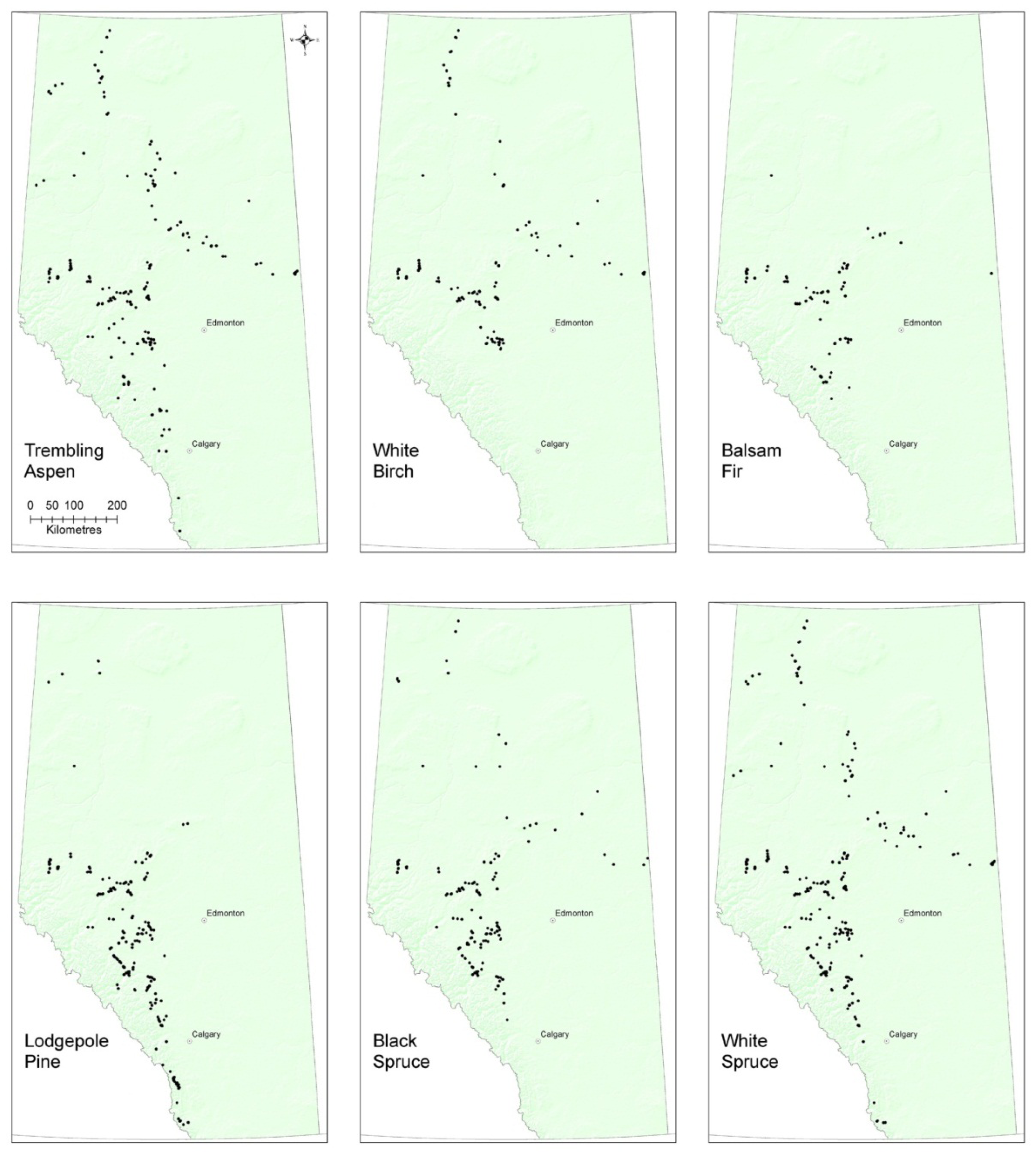
The data used for this study comes from the Alberta Government's Permanent Sample Plots (PSPs) located across the province of Alberta (Figure 1). The tree species were selected based on the number of sampled trees available by excluding those species with less than 1000 observations. The selected species are: two broadleaves including trembling aspen (Populus tremuloides Michx.) and white birch (Betula papyrifera Marsh.); and four conifers including balsam fir (Abies balsamea (L.) Mill.), lodgepole pine (Pinus contorta Dougl.), black spruce (Picea mariana (Mill.) B.S.P.), and white spruce (Picea glauca (Moench) Voss).
According to the ‘2005 PSP Field Procedure Manual’ [16], height to live crown is that point that divides a portion of the tree that is continuously branched from another part that has sporadic or no branching. For broadleaf trees the live crown starts at the lowest leaves level and not at the branch level. Crown width measurements are taken in the four cardinal directions (i.e., North, West, South and East) at the widest portion of the foliage for each direction by looking up from the base of the tree. Crown attributes such as crown area (CA), crown volume (CV), and crown surface area (CSA) were then calculated assuming a prolate ellipsoid shape for the broadleaves, and a conical shape for the conifers. Crown radii were not measured for each tree in the plot; therefore crown attributes of competing vegetation could not be used as an estimate of competition.
In order to quantify the effect of competition, we calculated: basal area per hectare (BA), number of trees per hectare (TN), and basal area of the larger trees per hectare (BALT). BALT is the basal area sum of each tree larger than the subject tree (within the plot). For each species and PSP only the last available measurement was used for the analysis. Table 1 for the broadleaves and Table 2 for the conifers, provide basic statistical information (e.g., mean and standard deviation) for a number of representative variables such as plot size, DBH, height, and crown and stand attributes.
We also calculated a number of selected climate variables using the spatial climate model ClimateWNA [17] that provided monthly data for each site based on latitude, longitude and elevation [15]. For the climate normal period 1971–2000, we calculated climate data for five representative climate variables including: MSP = Mean annual Summer (May to September) Precipitation (mm); AH:M = Annual Heat:Moisture index (i.e., (Mean Annual Temperature + 10)/(Mean Annual Precipitation/1000)); SH:M = Summer Heat:Moisture index (i.e., (Mean Warmest Month Temperature)/(MSP/1000)); DD > 5 = Degree-Days above 5 °C (i.e., growing degree-days); and CMD = Hargreaves Climatic Moisture Deficit [18]. Table 3 provides basic statistical information (e.g., mean and standard deviation) for each climate variable.
2.2. Model Selection
During the preliminary analysis we screened several non-linear candidate equations to investigate the relationship between diameter and height. We compared the models using several criteria such as the coefficient of determination (R2), the root mean squared error (RMSE), and the Akaike's information criterion (AIC), which quantifies the tradeoff between bias and variance in model construction. The following models fitted the data well:
DBH was measured at 1.3 m; however we decided to also include in the models those trees that are 1.3 m tall by using height minus 1.29 m for the analysis.
The relationship between diameter (i.e., DBH) and crown attributes (i.e., crown radius, crown length, crown area, crown volume, crown surface area) was then tested using the following model selected during preliminary analysis:
Analysis indicated that crown volume and crown length were the best predictors (lower AIC) of diameter for the six tree species. However, considering that crown area also performed well, and is easily determined from LiDAR or aerial photos we decided to use this variable in subsequent analysis. Thus crown area (CA) was added to Equations (1) and (2) as follows:
Preliminary analysis also included F-ratio tests [19] to compare Equation (1) with Equation (2); and Equation (4) with Equation (5). The results indicated that Equation (4) was the best model (lowest AIC) for trembling aspen and white birch; and Equation (5) was the best model (lowest AIC) for balsam fir, lodgepole pine, black spruce and white spruce.
During the preliminary analysis we also included stand and tree attributes such as basal area per hectare (BA), the number of trees per hectare (TN), and, at the tree level, basal area of the larger trees per hectare (BALT) into the model. The results indicated that BALT had the highest predictive ability (lowest AIC). F-ratio tests were then carried out to investigate if the inclusion of BALT improved the overall predictive ability (lower AIC) compared to models without the stand attribute. The results provided evidence that including BALT significantly improved the model fit and was therefore included in the base models as follows:
2.3. Natural Sub-Region, Moisture and Nutrient Regimes, and Climate
Natural Sub-Region (NSR) [14] and moisture and nutrient regimes [20] were separately added to the models using indicator variables (i.e., zi*di; where di is the indicator variable 1 if NSR, 0 otherwise, and zi is the NSR parameter) [19]. The NSRs include the Central Mixedwood, the Dry Mixedwood, the Lower Boreal Highlands, the Lower Foothills, the Montane, the Northern Mixedwood, the Subalpine, and the Upper Foothills [21]. The moisture regimes (i.e., 2–9) were grouped into low, medium, and high levels of moisture (i.e., Low = 2, 3, and 4; Medium = 5 and 6; High = 7, 8, and 9), and the nutrient regimes (i.e., 1–5) were grouped into low, medium, and high levels (i.e., Low = 1 and 2; Medium = 3; High = 4 and 5).
For trembling aspen and white birch the equation tested is:
For balsam fir, lodgepole pine, black spruce and white spruce the equation tested is:
F-ratio tests were then used to investigate if two or more NSRs could be grouped together, and to test if the inclusion of NSR, and moisture and nutrient regimes overall improved the predictive ability of the base model.
Then we tested the inclusion of five representative climate variables (Clim. Var.) such as MSP, AH:M, SH:M, DD > 5, and CMD. For trembling aspen and white birch the equation tested is:
For balsam fir, lodgepole pine, black spruce and white spruce the equation tested is:
2.4. Mixed Model Analysis
In order to account for the nested sources of variability related to plot, preliminary analysis of mixed effect models including plot as a random subject in Equations (8) and (9) was carried out. For each species, best results were obtained for models with only one random parameter (b0 added to the slope β0). Mixed effect models with more than one random parameter either failed to converge or resulted in non-significant estimates, likely owing to the relatively small number of trees in some PSPs. These models were then tested with and without the inclusion of NSR information (i.e., zi*di). For trembling aspen and white birch the equations tested are:
For balsam fir, lodgepole pine, black spruce and white spruce the equations tested are:
Parameter estimation for both fixed-effects and mixed-effects models was completed using the NLMIXED procedure in SAS statistical package [22].
3. Results
The base model that included Ht, crown area and BALT accounted for much of the variation in DBH (R2 from 0.858 to 0.937) and resulted in RMSE ranging from 4.6 to 2.0 cm (Table 4). Including NSR information into the base models significantly improved the model fit for all six species (Table 5). F-ratio tests indicated that grouping three NSRs (i.e., Central Mixedwood, Dry Mixedwood and Northern Mixedwood) reduced AIC for trembling aspen, but grouping NSRs increased AIC for the remaining species.
The inclusion of moisture regime resulted in parameters significantly different from zero (α = 0.05) only for trembling aspen and white spruce. However, moisture regime did not improve the overall fit (resulting in higher AIC) compared to models with NSR information. Adding nutrient regime into the model again resulted in parameters significantly different from zero (α = 0.05) for trembling aspen and white spruce. Inclusion of nutrient regime improved the model fit only for trembling aspen as compared to the model with the NSR information, but not for white spruce.
Adding climate variables to the models resulted in a better fit for trembling aspen, lodgepole pine, and black spruce compared to models with NSR information (Table 6). For balsam fir there was no significant difference between the two models, and for white birch and white spruce the models with the NSRs provided slightly better fit than the models with the climate variables.
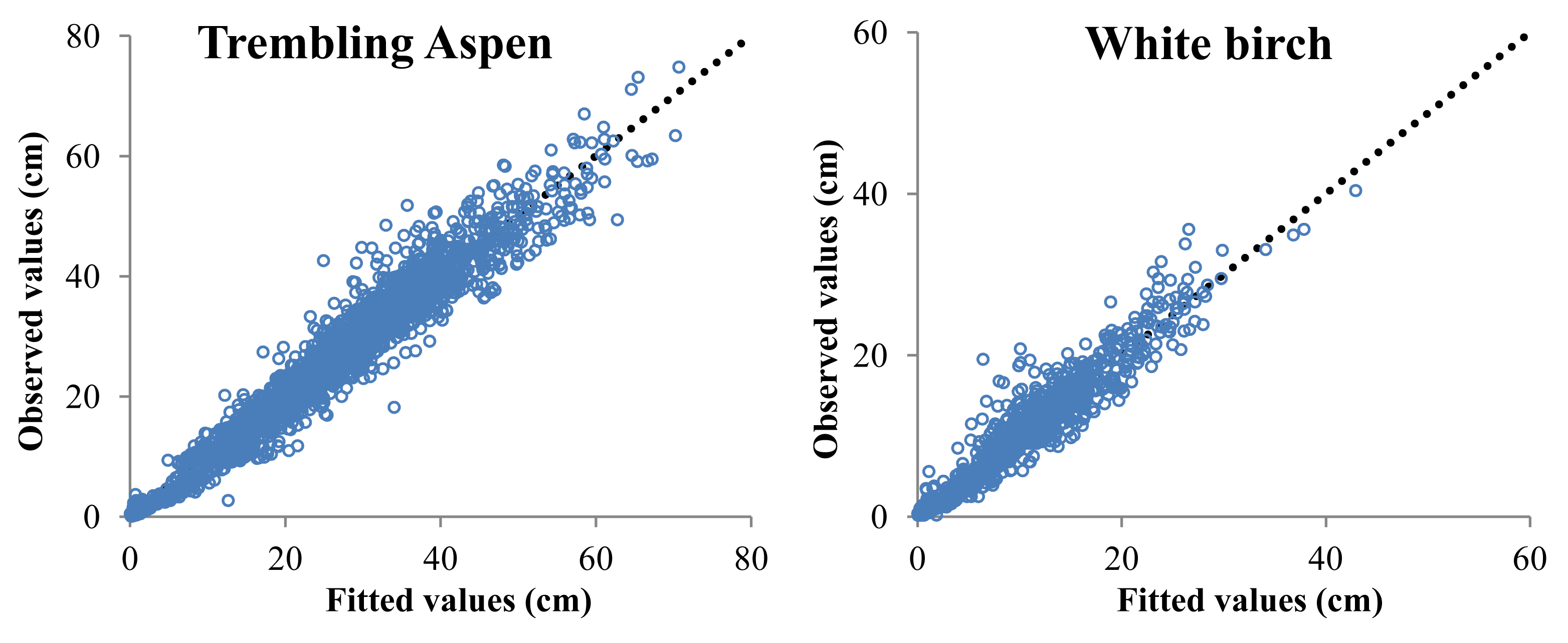
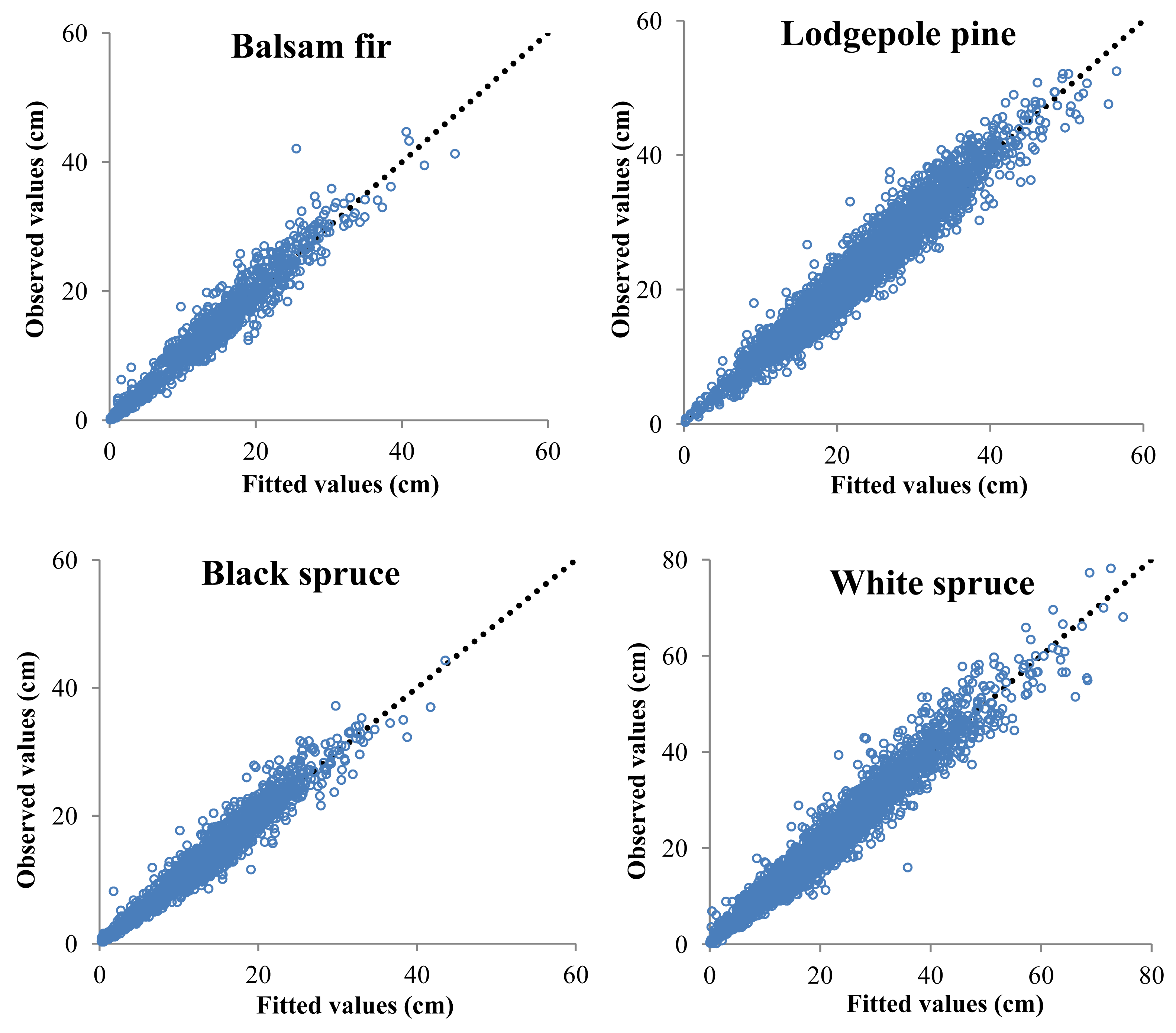
The results from the mixed model analysis indicate that by adding plot as a random subject, the overall fit of the model improved compared to fixed effect models only (Tables 7 and 8; and Figure 2). However, mixed effect models resulted in only minor improvements for models with NSR information.
where yi —observed values; ŷi —predicted values; ȳ —average; n—sample size; k—number of model parameters; ln(L)—logarithm of the likelihood function.
4. Discussion
The analysis confirmed that non-linear models best represent the relationship between diameter and height [23]. The base models were significantly improved by the addition of crown area and basal area of the larger trees. These measures are linked to the tree competitive status and the availability of resources during the growing season [24], which may have a stronger influence on stem diameter than on tree height.
The fit of models was also improved by including both NSRs and climate but the inclusion of nutrient and moisture regimes was not beneficial. Other studies have shown that climatic variables can be used to improve the predictive ability of growth models [13,25] and are particularly effective for retrospective analysis including short-term updates of forest inventory [26].
The similar results obtained with climate variables and the NSRs are likely related to the strong influence of climate in defining these ecological units which are also based on landscape patterns (e.g., vegetation), soils and physiographic features [14]. Given the relatively narrow range of variability between sites in terms of moisture and nutrient regime estimates, these factors proved to have low predictive ability when added to the base models.
Grouping NSRs significantly improved model performance only for trembling aspen. This species has an extensive range and is able to grow on a variety of climates and soils [27], which may explain the possibility to group more NSRs together within the diameter model. However, trembling aspen is considered relatively sensitive to drought [28] and, considering the current warming trend [29], diameter models that account for the climatic factors should be preferred.
Accounting for nested sources of variability (e.g., plot) using mixed models further improved the diameter model fit and provided RMSE values between 1.57 and 2.84 cm, which is between 8.9 and 19.8% of average diameter. A similar study using non-linear models for conifer species in Canada have indicated RMSE values between 2.4 and 3.6 cm [30]. Recent studies have also shown that mixed-effects models are preferred for models of height and diameter [31-33].
The diameter models developed indicated that Natural Sub-Regions and climate indices (e.g., Annual Heat:Moisture index) are important factors to be considered in fixed effects diameter models, while mixed effects models are able to produce accurate diameter estimates when the variability related to plot location is taken into account. In this regard, the mixed effect models might be preferable for retrospective analysis including short-term updates of forest inventory [26], while fixed effect models with climate related variables may be more useful when investigating the relationship between diameter and height in relation to existing climate gradients across Alberta.
Several previous studies on models predicting height from diameter (e.g., [34]) indicated that the inclusion of other tree and stand parameters improves the model fit. Moreover, the asymptotic relationship between height and diameter provides for additional complexity; at the same time, it was documented that models of height and diameter are more strongly asymptotic for individual stands than for regional models [35]. While crown measures and social status may improve model fits, these attributes may also be influenced by factors such as stand age and structure, as well as site conditions. However, in our study the inclusion of site attributes (moisture and nutrient regime) did not result in a significant improvement of model prediction; comparatively the regional variation (represented in the models by the Natural Sub-Regions) provided superior predictions.
The developed models can provide accurate estimates of diameter at a regional level (i.e., province of Alberta), but further studies should aim at expanding their applicability to the entire range of each tree species in order to provide generally applicable models of diameter and height. A potential issue in model application is that ground-measured tree and stand characteristics were used in model fitting. As it becomes operationally feasible to estimate these tree and stand characteristics through remote sensing techniques, it will also be possible to assess differences between ground-based and remote sensing-based estimates of the predictor variable [36]. It may be necessary to develop calibration functions to adjust any biases in the remote sensing-based estimates. In a remote sensing environment, the parameter related to the estimate of competition represented in the models by basal area of the larger trees should be recalculated by using instead crown area of competing vegetation. Crown attributes of individual trees can be derived by combining LiDAR data with aerial photographs or high resolution multispectral imagery [37].
5. Conclusions
The mixed models developed in this study provide accurate estimates of stem diameter based on height, crown area and basal area of the larger trees for several species in Alberta. Overall, the models are able to explain 95% of the variation in diameter at breast height across the six species with a root mean square error of 2.0 cm (13.4% of mean diameter). Fixed effect models with the inclusion of Natural Sub-Region (NSR) information are able to explain 90% of the variation in diameter at breast height across the six species with a root mean square error equal to 2.8 cm (17.9% of mean diameter). Selected climate variables provided similar results to models with NSR information. These models are a step forward in allowing the prediction of stem diameter at regional level using measurements of height and crown area provided by remote sensing.


| Species | Variable | Minimum | Mean | Maximum | Standard Deviation |
|---|---|---|---|---|---|
| Plots size (ha) | 0.02 | 0.13 | 0.20 | 0.05 | |
| Trembling aspen (Aw) PSPs: 194 Observations: 2791 | DBH (cm) | 0.1 | 24.0 | 74.8 | 13.4 |
| HT (m) | 1.3 | 20.3 | 37.2 | 7.4 | |
| CR (m) | 0.1 | 1.8 | 6.0 | 0.9 | |
| CL (m) | 0.1 | 5.7 | 16.5 | 2.6 | |
| CA (m2) | 0.1 | 13.5 | 112.0 | 13.3 | |
| BA (m2 ha−1) | 6.8 | 39.8 | 94.2 | 12.6 | |
| BALT (m2 ha−1) | 0.0 | 23.0 | 94.2 | 14.6 | |
| Plot size (ha) | 0.02 | 0.14 | 0.20 | 0.05 | |
| White birch (Bw) PSPs:113 Observations: 1351 | DBH (cm) | 0.2 | 9.3 | 40.4 | 6.8 |
| HT (m) | 1.3 | 9.7 | 26.5 | 5.3 | |
| CR (m) | 0.1 | 1.4 | 5.2 | 0.7 | |
| CL (m) | 0.1 | 5.1 | 15.4 | 3.1 | |
| CA (m2) | 0.1 | 7.7 | 84.9 | 7.4 | |
| BA (m2 ha−1) | 6.8 | 38.1 | 106.8 | 12.6 | |
| BALT (m2 ha−1) | 2.4 | 36.2 | 106.8 | 13.2 | |
| Species | Variable | Minimum | Mean | Maximum | Standard Deviation |
|---|---|---|---|---|---|
| Plot size (ha) | 0.04 | 0.13 | 0.20 | 0.05 | |
| Balsam fir (Fb) PSPs: 88 Observations: 1507 | DBH (cm) | 0.1 | 11.0 | 44.7 | 8.2 |
| HT (m) | 1.3 | 9.7 | 29.2 | 6.5 | |
| CR (m) | 0.1 | 1.2 | 3.0 | 0.5 | |
| CL (m) | 0.1 | 5.7 | 24.5 | 4.0 | |
| CA (m2) | 0.1 | 5.3 | 28.7 | 4.3 | |
| BA (m2 ha−1) | 10.3 | 41.6 | 106.8 | 12.9 | |
| BALT (m2 ha−1) | 0.0 | 38.4 | 106.5 | 14.1 | |
| Plot size (ha) | 0.02 | 0.09 | 0.20 | 0.05 | |
| Lodgepole pine (Pl) PSPs: 230 Observations: 5450 | DBH (cm) | 0.3 | 21.2 | 52.5 | 8.2 |
| HT (m) | 1.4 | 19.2 | 34.4 | 5.7 | |
| CR (m) | 0.1 | 1.2 | 3.5 | 0.5 | |
| CL (m) | 0.1 | 5.4 | 19.2 | 2.4 | |
| CA (m2) | 0.1 | 5.4 | 39.6 | 4.8 | |
| BA (m2 ha−1) | 1.1 | 45.3 | 125.0 | 15.0 | |
| BALT (m2 ha−1) | 0.0 | 24.5 | 107.0 | 14.9 | |
| Plot size (ha) | 0.02 | 0.09 | 0.20 | 0.05 | |
| Black spruce (Sb) PSPs: 155 Observations: 2380 | DBH (cm) | 0.3 | 13.6 | 44.3 | 6.3 |
| HT (m) | 1.4 | 12.4 | 32.0 | 5.0 | |
| CR (m) | 0.1 | 1.0 | 3.5 | 0.4 | |
| CL (m) | 0.3 | 7.0 | 23.8 | 4.1 | |
| CA (m2) | 0.1 | 3.9 | 38.8 | 3.3 | |
| BA (m2 ha−1) | 0.7 | 44.2 | 125.0 | 20.6 | |
| BALT (m2 ha−1) | 0.0 | 34.6 | 124.1 | 19.0 | |
| Plot size (ha) | 0.02 | 0.13 | 0.20 | 0.06 | |
| White spruce (Sw) PSPs: 249 Observations: 4450 | DBH (cm) | 0.2 | 19.4 | 78.2 | 11.9 |
| HT (m) | 1.3 | 15.8 | 39.1 | 8.1 | |
| CR (m) | 0.1 | 1.4 | 5.2 | 0.6 | |
| CL (m) | 0.2 | 9.1 | 33.2 | 5.1 | |
| CA (m2) | 0.1 | 7.7 | 84.1 | 6.7 | |
| BA (m2 ha−1) | 1.1 | 41.9 | 94.2 | 11.6 | |
| BALT (m2 ha−1) | 0.0 | 31.3 | 89.4 | 15.2 | |
| Species | Variable | Minimum | Mean | Maximum | Standard Deviation |
|---|---|---|---|---|---|
| MSP (mm) | 226.0 | 362.5 | 485.0 | 67.1 | |
| Trembling aspen (Aw) | AH:M | 14.5 | 21.7 | 25.6 | 1.6 |
| SH:M | 23.9 | 43.5 | 72.7 | 11.4 | |
| DD > 5 | 361.0 | 1188.8 | 1423.0 | 130.3 | |
| CMD | 2.0 | 118.4 | 234.0 | 61.0 | |
| MSP (mm) | 226.0 | 384.4 | 493.0 | 67.1 | |
| White birch (Bw) | AH:M | 17.7 | 21.4 | 25.6 | 1.1 |
| SH:M | 23.9 | 40.7 | 73.1 | 11.4 | |
| DD > 5 | 361.0 | 1182.8 | 1677.0 | 128.2 | |
| CMD | 22.0 | 100.0 | 262.0 | 58.0 | |
| MSP (mm) | 310.0 | 426.1 | 511.0 | 31.4 | |
| Balsam fir (Fb) | AH:M | 14.1 | 19.9 | 25.6 | 1.7 |
| SH:M | 25.7 | 33.7 | 54.6 | 3.9 | |
| DD > 5 | 640.0 | 1105.5 | 1385.0 | 146.3 | |
| CMD | 0.0 | 54.5 | 195.0 | 24.4 | |
| MSP (mm) | 251.0 | 422.4 | 575.0 | 36.5 | |
| Lodgepole pine (Pl) | AH:M | 8.9 | 19.2 | 25.3 | 2.5 |
| SH:M | 22.3 | 33.2 | 63.9 | 5.1 | |
| DD > 5 | 640.0 | 1049.5 | 1891.0 | 197.1 | |
| CMD | 0.0 | 61.2 | 261.0 | 41.1 | |
| MSP (mm) | 229.0 | 415.9 | 575.0 | 48.8 | |
| Black spruce (Sb) | AH:M | 14.5 | 20.3 | 25.1 | 1.5 |
| SH:M | 23.6 | 35.1 | 70.4 | 7.5 | |
| DD > 5 | 640.0 | 1100.0 | 1549.0 | 126.4 | |
| CMD | 2.0 | 69.1 | 224.0 | 40.4 | |
| MSP (mm) | 226.0 | 387.5 | 575.0 | 69.0 | |
| White spruce (Sw) | AH:M | 14.1 | 20.6 | 25.6 | 2.0 |
| SH:M | 23.6 | 39.4 | 73.1 | 11.7 | |
| DD > 5 | 361.0 | 1117.7 | 1891.00 | 160.0 | |
| CMD | 0.0 | 90.5 | 262.0 | 63.1 | |
| Spp. | βo | β1 | β2 | β3 | β4 | R2 | RMSE cm | AIC |
|---|---|---|---|---|---|---|---|---|
| Aw | 1.0691 (0.548) | 1.0066 (0.171) | - | 0.1681 (0.005) | −0.1016 (0.003) | 0.883 | 4.567 | 16410 |
| Bw | 1.6998 (0.097) | 0.7918 (0.021) | - | 0.2339 (0.012) | −0.1262 (0.011) | 0.883 | 2.328 | 6123.7 |
| Fb | 3.5636 (0.161) | 0.7496 (0.274) | 1.0014 (0.002) | 0.1019 (0.006) | −0.1716 (0.005) | 0.937 | 2.054 | 6461.5 |
| Pl | 3.3821 (0.223) | 0.5803 (0.035) | 1.0122 (0.002) | 0.128 (0.003) | −0.08618 (0.002) | 0.858 | 3.081 | 27739 |
| Sb | 3.0794 (0.155) | 0.6881 (0.032) | 1.0051 (0.002) | 0.148 (0.004) | −0.1159 (0.142) | 0.878 | 2.220 | 10558 |
| Sw | 2.2699 (0.108) | 0.8587 (0.025) | 0.9973 (0.001) | 0.1372 (0.003) | −0.1134 (0.002) | 0.924 | 3.269 | 23178 |
| Spp. | β0 | β1 | β2 | β3 | β4 | z1 | z2 | z3 | z4 | z5 | z6 | z7 | z8 | R2 | RMSE cm | AIC |
|---|---|---|---|---|---|---|---|---|---|---|---|---|---|---|---|---|
| CM,DMW, NM | LF,UF | LBH | M | |||||||||||||
| Aw | 1.0399 (0.053) | 1.0187 (0.017) | - | 0.1643 (0.005) | −0.1001 (0.003) | −0.06211 (0.022) | 0.02761 (0.014) | −0.1366 (0.020) | 0.2536 (0.061) | - | - | - | - | 0.887 | 4.501 | 16328 |
| CM | DMW | LBH | LF | M | NM | SA | UF | |||||||||
| Bw | 0.9024 (0.099) | 0.7962 (0.021) | - | 0.2296 (0.012) | −0.146 (0.012) | 0.8119 (0.027) | 1.2869 (0.075) | 0.9264 (0.050) | 0.9469 (0.026) | - | 0.9965 (0.053) | - | 1.1339 (0.097) | 0.889 | 2.279 | 6071.6 |
| Fb | 2.7672 (0.121) | 0.7573 (0.026) | 0.9981 (0.002) | 0.1082 (0.007) | -0.1613 (0.005) | 0.4391 (0.054) | - | - | 0.6233 (0.041) | - | - | 0.9414 (0.106) | 0.9634 (0.054) | 0.943 | 1.955 | 6308.4 |
| Pl | 1.7948 (0.182) | 0.607 (0.036) | 1.0133 (0.002) | 0.1322 (0.003) | −0.0826 (0.002) | 1.1679 (0.042) | - | 1.2455 (0.054) | 1.1445 (0.027) | 1.2458 (0.043) | - | 1.5493 (0.053) | 1.2418 (0.035) | 0.864 | 3.019 | 27522 |
| Sb | 2.0392 (0.139) | 0.6568 (0.031) | 1.0088 (0.002) | 0.1464 (0.004) | −0.1258 (0.004) | 1.0179 (0.047) | - | 0.9587 (0.056) | 1.1891 (0.041) | - | 1.0313 (0.145) | 2.2039 (0.139) | 1.4383 (0.050) | 0.888 | 2.123 | 10351 |
| Sw | 1.1818 (0.093) | 0.8231 (0.024) | 1.0007 (0.001) | 0.1383 (0.003) | −0.1068 (0.002) | 1.003 (0.016) | 1.08 (0.023) | 0.948 (0.024) | 1.1393 (0.017) | 1.2308 (0.069) | 1.0124 (0.025) | 1.3077 (0.046) | 1.2605 (0.024) | 0.930 | 3.153 | 22863 |
CM = Central Mixedwood; DMW = Dry Mixedwood; LBH = Lower Boreal Highlands; LF = Lower Foothills; M = Montane; NM = Northern Mixedwood; SA = Subalpine; UF = Upper Foothills.
| Species | β0 | β1 | β2 | β3 | β4 | β5 | R2 | RMSE cm | AIC | |
|---|---|---|---|---|---|---|---|---|---|---|
| Climate Variable | Value | |||||||||
| Aw | 3.3598 (0.247) | 0.9965 (0.016) | - | 0.1523 (0.005) | −0.09566 (0.003) | SH:M | −0.2942 (0.015) | 0.899 | 4.259 | 16016 |
| Bw | 7.0926 (2.19) | 0.8075 (0.021) | - | 0.2275 (0.012) | −0.1363 (0.012) | AH:M | −0.4633 (0.099) | 0.885 | 2.311 | 6103.9 |
| Fb | 16.3002 (2.006) | 0.7491 (0.026) | 0.9998 (0.002) | 0.1169 (0.006) | −0.1561 (0.005) | AH:M | −0.5306 (0.041) | 0.943 | 1.950 | 6297.3 |
| Pl | 7.9248 (0.615) | 0.602 (0.035) | 1.0145 (0.002) | 0.1341 (0.003) | −0.08093 (0.002) | AH:M | −0.3323 (0.016) | 0.867 | 2.976 | 27361 |
| Sb | 26.7343 (3.295) | 0.6652 (0.030) | 1.0092 (0.002) | 0.1419 (0.004) | −0.1106 (0.004) | AH:M | −0.7204 (0.038) | 0.893 | 2.081 | 10250 |
| Sw | 3.7607 (0.209) | 0.8449 (0.024) | 0.9993 (0.001) | 0.1301 (0.003) | −0.1087 (0.002) | SH:M | −0.1383 (0.009) | 0.929 | 3.175 | 22920 |
AH:M = annual heat:moisture index (MAT + 10)/(MAP/1000)); SH:M = summer heat:moisture index ((MWMT)/(MSP/1000)).
| Spp. | Eq. | β0 | β1 | β2 | β3 | β4 | z1 | z2 | z3 | z4 | Z5 | Z6 | Z7 | Z8 | σ2b0 |
|---|---|---|---|---|---|---|---|---|---|---|---|---|---|---|---|
| CM,DMW,NM | LF,UF | LBH | M | ||||||||||||
| Aw | (12) | 2.0276 (0.105) | 0.8787 (0.016) | - | 0.09918 (0.004) | −0.135 (0.003) | NS | NS | −0.2191 (0.108) | NS | - | - | - | - | 0.09835 |
| Aw | (13) | 2.0579 (0.104) | 0.875 (0.016) | - | 0.09925 (0.004) | −0.1353 (0.003) | - | - | - | - | - | - | - | - | 0.1068 |
| CM | DMW | LBH | LF | M | NM | SA | UF | ||||||||
| Bw | (12) | 1.7101 (0.173) | 0.7842 (0.021) | - | 0.2253 (0.011) | −0.2264 (0.014) | 0.6924 (0.083) | 1.3265 (0.270) | 0.8159 (0.178) | 0.7992 (0.077) | - | 0.9374 (0.155) | - | 1.0589 (0.206) | 0.08388 |
| Bw | (13) | 2.4834 (0.176) | 0.7837 (0.021) | - | 0.2252 (0.011) | −0.2249 (0.014) | - | - | - | - | - | - | - | - | 0.09462 |
| Fb | (14) | 2.688 (0.122) | 0.7027 (0.024) | 1.004 (0.002) | 0.1229 (0.007) | −0.1453 (0.007) | 0.3801 (0.091) | - | - | 0.5904 (0.061) | - | - | 1.0289 (0.158) | 0.8888 (0.077) | 0.05267 |
| Fb | (15) | 3.3503 (0.147) | 0.6983 (0.024) | 1.0045 (0.002) | 0.1232 (0.007) | −0.1445 (0.007) | - | - | - | - | - | - | - | - | 0.08101 |
| Pl | (14) | 1.3209 (0.126) | 0.9433 (0.033) | 0.987 (0.002) | 0.09031 (0.002) | −0.1136 (0.002) | 0.9713 (0.094) | - | 0.9633 (0.162) | 0.8947 (0.048) | 0.736 (0.084) | - | 1.0486 (0.068) | 0.9126 (0.051) | 0.09937 |
| Pl | (15) | 2.2224 (0.142) | 0.9475 (0.033) | 0.9867 (0.002) | 0.09017 (0.002) | −0.1137 (0.002) | - | - | - | - | - | - | - | - | 0.1026 |
| Sb | (14) | 1.6678 (0.131) | 0.8271 (0.029) | 0.9941 (0.002) | 0.1079 (0.005) | −0.1393 (0.005) | 1.0231 (0.102) | - | 0.944 (0.119) | 1.1825 (0.074) | - | 0.9064 (0.219) | 2.013 (0.284) | 1.3988 (0.081) | 0.09419 |
| Sb | (15) | 2.879 (0.141) | 0.8342 (0.029) | 0.9935 (0.002) | 0.1067 (0.005) | −0.1395 (0.005) | - | - | - | - | - | - | - | - | 0.1195 |
| Sw | (14) | 1.1411 (0.082) | 0.8459 (0.021) | 0.9987 (0.001) | 0.1215 (0.004) | −0.1043 (0.002) | 1.0105 (0.041) | 1.1182 (0.093) | 0.919 (0.079) | 1.1432 (0.037) | 1.1946 (0.133) | 1.0319 (0.091) | 1.2969 (0.110) | 1.2267 (0.044) | 0.04576 |
| Sw | (15) | 2.2705 (0.089) | 0.8465 (0.021) | 0.9986 (0.001) | 0.1208 (0.004) | −0.1048 (0.002) | - | - | - | - | - | - | - | - | 0.0544 |
| Mixed Effect Models | Fixed Effect Models | |||||||||||
|---|---|---|---|---|---|---|---|---|---|---|---|---|
| Spp. | Eq. | Par | R2 | RMSE cm | RMSE % | AIC | Equation | Par | R2 | RMSE cm | RMSE % | AIC |
| Aw | (12) | 9 | NS* | NS* | NS * | NS * | (8) | 8 | 0.887 | 4.501 | 18.8 | 16328 |
| Aw | (13) | 5 | 0.955 | 2.838 | 11.8 | 14499 | ||||||
| Bw | (12) | 11 | 0.927 | 1.849 | 19.9 | 5748.5 | (8) | 10 | 0.889 | 2.279 | 24.5 | 6071.6 |
| Bw | (13) | 5 | 0.927 | 1.842 | 19.8 | 5744 | ||||||
| Fb | (14) | 10 | 0.956 | 1.713 | 15.6 | 6070.8 | (9) | 9 | 0.943 | 1.955 | 17.8 | 6308.4 |
| Fb | (15) | 6 | 0.956 | 1.709 | 15.5 | 6087.6 | ||||||
| Pl | (14) | 12 | 0.947 | 1.890 | 8.9 | 23508 | (9) | 11 | 0.864 | 3.019 | 14.2 | 27522 |
| Pl | (15) | 6 | 0.947 | 1.889 | 8.9 | 23505 | ||||||
| Sb | (14) | 12 | 0.938 | 1.577 | 11.6 | 9411.1 | (9) | 11 | 0.888 | 2.123 | 15.6 | 10351 |
| Sb | (15) | 6 | 0.939 | 1.573 | 11.6 | 9427.5 | ||||||
| Sw | (14) | 14 | 0.956 | 2.488 | 12.8 | 21426 | (9) | 13 | 0.930 | 3.153 | 16.3 | 22863 |
| Sw | (15) | 6 | 0.956 | 2.484 | 12.8 | 21438 | ||||||
*NS = Some parameter values are not significantly different from zero (α = 0.05).
Acknowledgments
Special thanks go to Dave Morgan of the Alberta Sustainable Resource Development (SRD) for providing the Permanent Sample Plot data and the Canadian Wood Fibre Centre for funding of this research. We would like to thank also Gurp Thandi of the Canadian Forest Service for creating the maps presented in this manuscript.
References
- Avery, T.A.; Burkhart, H.E. Forest Measurements, 5th ed.; Mcgraw-Hill: New York, NY, USA, 2002; p. 456. [Google Scholar]
- Pitt, D.; Pineau, J. Forest inventory research at the Canadian Wood Fibre Centre: Notes from a research coordination workshop, 3–4 June, 2009, Pointe Claire, QC, Canada. For. Chron. 2009, 85, 859–869. [Google Scholar]
- Hudak, A.T.; Evans, J.S.; Smith, A.M.S. LiDAR utility for natural resources managers. Remote Sens. 2009, 1, 934–951. [Google Scholar]
- Woods, M.; Lim, K.; Treits, P. Predicting forest stand variables from LiDAR data in the Great Lakes—St. Lawrence forest of Ontario. For. Chron. 2008, 84, 827–839. [Google Scholar]
- Thomas, V.; Oliver, R.D.; Lim, K.; Woods, M. LiDAR and Weibull modeling of diameter and basal area. For. Chron. 2008, 84, 866–875. [Google Scholar]
- Morsdorf, F.; Kötz, B.; Meier, E.; Itten, K.I.; Allgöwer, B. Estimation of LAI and fractional cover from small footprint airborne laser scanning data based on gap fraction. Remote Sens. Environ. 2006, 104, 50–61. [Google Scholar]
- Næsset, E.; Gobakken, T. Estimation of above- and below-ground biomass across regions of the boreal forest zone using airborne laser. Remote Sens. Environ. 2008, 112, 3079–3090. [Google Scholar]
- Lefsky, M.; McHale, M.R. Volume estimates of trees with complex architecture from terrestrial laser scanning. J. Appl. Remote Sens. 2008, 2, 023521:1–023521:19. [Google Scholar]
- Zagalikis, G.; Cameron, A.D.; Miller, D.R. The application of digital photogrammetry and image analysis techniques to derive tree and stand characteristics. Can. J. For. Res. 2005, 35, 1224–1237. [Google Scholar]
- Wang, Y.; Titus, S.J.; LeMay, V.M. Relationships between tree slenderness coefficients and tree or stand characteristics for major species in boreal mixedwood forests. Can. J. For. Res. 1998, 28, 1171–1183. [Google Scholar]
- Rudnicki, M.; Silins, U.; Lieffers, V.J. Crown cover is correlated with relative density, tree slenderness, and tree height in lodgepole pine. For. Sci. 2004, 50, 356–363. [Google Scholar]
- Fish, H.; Lieffers, V.J.; Silins, U.; Hall, R.J. Crown shyness in lodgepole pine stands of varying stand height, density, and site index in the upper foothills of Alberta. Can. J. For. Res. 2006, 36, 2104–2111. [Google Scholar]
- Woollons, R.C.; Snowdon, P.; Mitchell, N.D. Augmenting empirical stand projection equations with edaphic and climatic variables. For. Ecol. Manag. 1997, 98, 267–275. [Google Scholar]
- Albert, A.; Pettapiece, W.W.; Downing, D.J. Natural Regions and Subregions of Alberta; Natural Regions Committee: Edmonton, AB, Canada, 2006. [Google Scholar]
- Wang, T.; Hamann, A.; Spittlehouse, D.L.; Aitken, S.N. Development of scale-free climate data for western Canada for use in resource management. Int. J. Climatol. 2006, 26, 383–397. [Google Scholar]
- Alberta Sustainable Resource Development. Permanent Sample Plot (PSP) Field Procedures Manual. Edmonton, AB, Canada. 2005. Available online: http://www.srd.alberta.ca/LandsForests/ForestManagement/PermanentSamplePlots/ (accessed on 28 August 2011).
- Mbogga, S.M.; Hamann, A.; Wang, T. Historical and projected climate data for natural resource management in western Canada. Agric. For. Meteorol. 2009, 149, 881–890. [Google Scholar]
- Hargreaves, G.H.; Samani, Z.A. Reference crop evaporation from temperature. Appl. Eng. Agric. 1985, 1, 96–99. [Google Scholar]
- Peng, C. Developing Ecoregion-based height diameter models for Jack pine and Black spruce in Ontario. For. Res. Rep. 2001, 159, 1–10. [Google Scholar]
- Beckingham, J.D.; Archibald, J.H. Field Guide to Ecosites of Northern Alberta; Canadian Forest Service, Northwest Region, Northern Forestry Centre: Edmonton, AB, Canada, 1996. [Google Scholar]
- Downing, D.J.; Pettapiece, W.W. Natural Regions and Subregions of Alberta; Natural Regions Committee, Government of Alberta: Edmonton, AB, Canada, 2006. [Google Scholar]
- SAS Statistical Package Version 9.2; SAS Institute Inc.: Cary, NC, USA, 2011.
- Parker, R.C.; Evans, D.L. An application of LiDAR in a double-sample forest inventory. West. J. Appl. For. 2004, 19, 95–101. [Google Scholar]
- Purves, D.W.; Lichstein, J.W.; Pacala, S.W. Crown plasticity and competition for canopy space: A new spatially implicit model parameterized for 250 North American tree species. PLoS One 2007, 2, e870. [Google Scholar]
- Snowdon, O.; Jovanovic, T.; Booth, T.H. Incorporation of indices of annual climatic variation into growth models for Pinus radiata. For. Ecol. Manag. 1999, 117, 187–197. [Google Scholar]
- Snowdon, P. Short-term predictions of growth of Pinus radiata with models incorporating indices of annual climatic variation. For. Ecol. Manag. 2001, 152, 1–11. [Google Scholar]
- Perala, D.A. Quacking aspen. In Silvics of North America: 2, Hardwoods; Burns, R.M., Honkala, B.H., Eds.; US Department of Agriculture: Washington, DC, USA, 1990. [Google Scholar]
- Hogg, E.H.; Brandt, J.P.; Michaelian, M. Impacts of a regional drought on the productivity, dieback, and biomass of western Canadian aspen forests. Can. J. For. Res. 2008, 38, 1373–1384. [Google Scholar]
- International Panel on Climate Change (IPCC). Climate Change 2007: Synthesis Report: Summary for Policymakers: An Assessment of the Intergovernmental Panel on Climate Change; IPCC: Valencia, Spain, 2007. [Google Scholar]
- Hall, R.J.; Wang, Y.; Morgan, D.J. Estimating tree diameter and volume with a taper model and large-scale photo measurements. North. J. Appl. For. 2001, 18, 110–118. [Google Scholar]
- Hall, D.B.; Bailey, R.L. Modeling and prediction of forest growth variables based on multilevel non-linear mixed models. For. Sci. 2001, 47, 311–321. [Google Scholar]
- Lynch, T.B.; Holley, A.G.; Stevenson, D.J. A random-parameter height-dbh model for cherrybark oak. South. J. Appl. For. 2005, 29, 22–26. [Google Scholar]
- Castedo Dorado, F.; Diéguez-Aranda, U.; Barrio Anta, M.; Sánchez Rodríguez, M.; Gadow, K. A generalized height-diameter model including random components for radiata pine plantations in northwestern Spain. For. Ecol. Manag. 2006, 229, 202–213. [Google Scholar]
- Sharma, M.; Parton, J. Height-diameter equations for boreal tree species in Ontario using a mixed-effects modeling approach. For. Ecol. Manag. 2007, 249, 187–198. [Google Scholar]
- Temesgen, H.; Hann, D.W.; Monleon, V.J. Regional height-diameter equations for major tree species of southwest Oregon. West. J. Appl. For. 2007, 22, 213–219. [Google Scholar]
- Vauhkonen, J.; Mehtätalo, L.; Packalén, P. Combining tree height samples produced by airborne laser scanning and stand management records to estimate plot volume in Eucalyptus plantations. Can. J. For. Res. 2011, 41, 1649–1658. [Google Scholar]
- Leckie, D.; Gougeon, F.; Hill, D.; Quinn, R.; Armstrong, L.; Shreenan, R. Combined high-density LiDAR and multispectral imagery for individual tree crown analysis. Can. J. Remote Sens. 2003, 29, 633–649. [Google Scholar]
- Conflict of Interest: The authors declare no conflict of interest.
© 2011 by the authors; licensee MDPI, Basel, Switzerland. This article is an open access article distributed under the terms and conditions of the Creative Commons Attribution license (http://creativecommons.org/licenses/by/3.0/).
Share and Cite
Cortini, F.; Filipescu, C.N.; Groot, A.; MacIsaac, D.A.; Nunifu, T. Regional Models of Diameter as a Function of Individual Tree Attributes, Climate and Site Characteristics for Six Major Tree Species in Alberta, Canada. Forests 2011, 2, 814-831. https://doi.org/10.3390/f2040814
Cortini F, Filipescu CN, Groot A, MacIsaac DA, Nunifu T. Regional Models of Diameter as a Function of Individual Tree Attributes, Climate and Site Characteristics for Six Major Tree Species in Alberta, Canada. Forests. 2011; 2(4):814-831. https://doi.org/10.3390/f2040814
Chicago/Turabian StyleCortini, Francesco, Cosmin N. Filipescu, Arthur Groot, Dan A. MacIsaac, and Thompson Nunifu. 2011. "Regional Models of Diameter as a Function of Individual Tree Attributes, Climate and Site Characteristics for Six Major Tree Species in Alberta, Canada" Forests 2, no. 4: 814-831. https://doi.org/10.3390/f2040814