Spatial Simulation Modelling of Future Forest Cover Change Scenarios in Luangprabang Province, Lao PDR

Abstract
: Taking Luangprabang province in Lao Peoples's Democratic Republic (PDR) as an example, we simulated future forest cover changes under the business-as-usual (BAU), pessimistic and optimistic scenarios based on the Markov-cellular automata (MCA) model. We computed transition probabilities from satellite-derived forest cover maps (1993 and 2000) using the Markov chains, while the “weights of evidence” technique was used to generate transition potential maps. The initial forest cover map (1993), the transition potential maps and the 1993–2000 transition probabilities were used to calibrate the model. Forest cover simulations were then performed from 1993 to 2007 at an annual time-step. The simulated forest cover map for 2007 was compared to the observed (actual) forest cover map for 2007 in order to test the accuracy of the model. Following the successful calibration and validation, future forest cover changes were simulated up to 2014 under different scenarios. The MCA simulations under the BAU and pessimistic scenarios projected that current forest areas would decrease, whereas unstocked forest areas would increase in the future. Conversely, the optimistic scenario projected that current forest areas would increase in the future if strict forestry laws enforcing conservation in protected forest areas are implemented. The three simulation scenarios provide a very good case study for simulating future forest cover changes at the subnational level (Luangprabang province). Thus, the future simulated forest cover changes can possibly be used as a guideline to set reference scenarios as well as undertake REDD/REDD+ preparedness activities within the study area.1. Introduction
Recent reports indicate that deforestation is the second largest source of greenhouse gas (GHG) emissions after the energy sector accounting for about 20% [1-3]. Given the growing awareness about the impact of GHG emissions on global climate change, a number of initiatives have been proposed in order to reduce deforestation and forest degradation, particularly in tropical countries. The REDD (Reducing Emissions from Deforestation and Forest Degradation) or REDD+ (which includes sustainable forest management and enhancement of forest carbon stocks) scheme is an example of such initiatives that are currently being negotiated under the United Nations Framework Convention on Climate Change (UNFCCC) to reduce emissions from deforestation and forest degradation in developing countries [4]. Under the REDD/REDD+ scheme, developing countries would receive incentives to reduce deforestation and the associated carbon emissions. REDD/REDD+ schemes are being considered as alternative mitigation options that could combat climate change as well as help to conserve biodiversity [2].
While REDD/REDD+ is seen as a low-cost option for mitigating climate change [5], its successful implementation requires the development of robust reference scenarios under the business-as-usual (BAU) conditions. A reference scenario (under BAU scenario) is the projected deforestation and the associated emissions in the absence of a REDD/REDD+ intervention scheme [4]. Several approaches for setting reference scenarios have been suggested, which include, among others, spatial and non-spatial modelling approaches [6-9]. In this paper, we focus on spatial simulation models because they provide visual and quantitative information that can be used to inform stakeholders how different policy options can affect forest cover changes as well as carbon emissions [10]. In addition, spatial simulation models have the potential to improve the quality of stakeholder negotiations on the REDD/REDD+ scheme since they also provide spatial forest cover change information under different simulation scenarios [11,12].
Although numerous spatial simulation models have provided valuable insights into forest cover change processes, particularly in the Amazon region [8,10,13,14], forest cover change dynamics are still poorly understood in South-east Asia, especially in areas under shifting cultivation systems [15,16]. This is mainly attributed to the fact that land use and forest cover changes exhibit high degrees of spatial and temporal complexity in tropical areas, which are influenced by various underlying driving factors [17]. In this regard, flexible spatial simulation models with the capacity to develop insights into forest cover change dynamics as well as explore “what if” scenarios (for forest cover changes) are required. The Markov-cellular automata (MCA) modelling approach can be used to gain insights into the current and future forest cover changes given its simplicity and flexibility. More importantly, the MCA model has the ability to model multidirectional land use and forest cover changes. For example, a landscape can change from either forest to non-forest or vice-versa. Furthermore, past studies have shown that the MCA models can be reliably used to simulate future land use and forest cover changes [10,13,15].
The objective of this study is to simulate future forest cover changes in the Luangprabang province, Lao People's Democratic Republic (PDR) under the business-as-usual (BAU), pessimistic (worst case) and optimistic (strict enforcement of forestry law) scenarios. The MCA model that integrates “weights of evidence” technique, Markov chains and cellular automata (CA) was used to simulate future forest cover changes up to 2014. The “weights of evidence” technique was used to compute transition potential maps based on biophyiscal and socioeconomic data such as “distance to major roads” and population density, while the Markov chains were used to generate the transition probabilities from the forest cover maps [10]. Transition potential maps represent the likelihood or the probability that the landscape would change from one forest cover class to another (e.g., forest to non-forest) whereas the transition probabilities represent the temporal changes among the forest cover classes. The cellular automata (CA) model functions were employed to simulate future forest cover changes based on the initial forest cover map (1993), transition potential maps and transition probabilities. Luangprabang province was thus selected because of the decrease of natural forest areas and the dominance of shifting cultivation, which is typical in the northern areas of Lao PDR [15].
2. Study Area
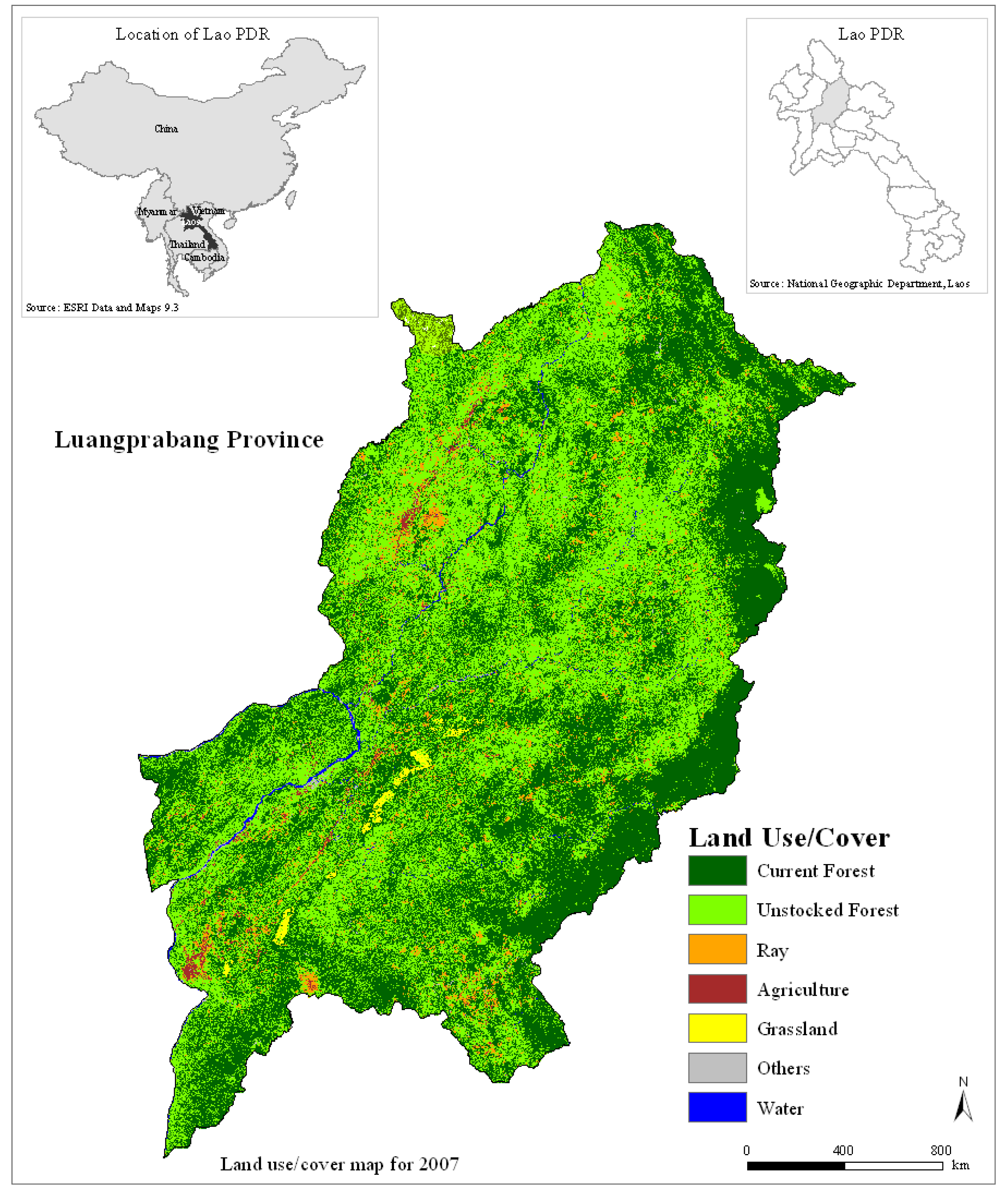
Luangprabang province is located in the northern part of Lao PDR (between 18°−21° N, 101°−104° E) (Figure 1). The province, covering an area of approximately 16,875 km2 is divided into 11 districts, namely Luangprabang, Xien Nguen, Nan, Park Ou, Nambak, Ngoi, Pakxeng, Phonxay, Chomphet, Viengkham and Phoukhoune [18]. The altitude of the study area varies approximately from 200 m to 2,257 m above sea level. According to the Lao Department of Statistics [18], the highest temperatures usually occur from March to October with a mean maximum temperature in the range of 30.9 °C to 33.5 °C. The study area receives about 2,104 mm of rainfall. Forest cover maps produced in 2002 by the Forest Inventory and Planning Division (FIPD) in Lao PDR show that Luangprabang province is dominated by unstocked forest covering approximately 60% of the province, while the upper mixed deciduous, ray and grassland occupy about 20%, 7% and 4% of the province, respectively. The “FAO Forest Resource Assessment” report [19] states that unstocked forest areas are previously forested areas in which the crown density has been reduced to less than 20% due to logging, shifting cultivation or other heavy disturbance; while ray is an area where the forest has been cut and burnt for the temporary cultivation of rice and other crops.
The total population in the province as of 2008 is approximately 431,439 inhabitants with a population density of 26 inhabitants/km2, which surpasses the country population density of 25 inhabitants/km2. Due to increasing population density and the fact that the majority of the people in the study area are dependent on agriculture for their livelihood, there has been a lot of pressure on the available forestry resources. The major economic activity in the province is subsistence agriculture. According to the 2008 agriculture statistics, the major crops produced in the province were maize (131,510 tonnes), starchy roots (106,475 tonnes), vegetables and beans (121,820 tonnes), rain-fed rice (48,205 tonnes), upland rice (21,820 tonnes), irrigated rice (9,270 tonnes), and other minor crops.
3. Methodology
3.1. Data
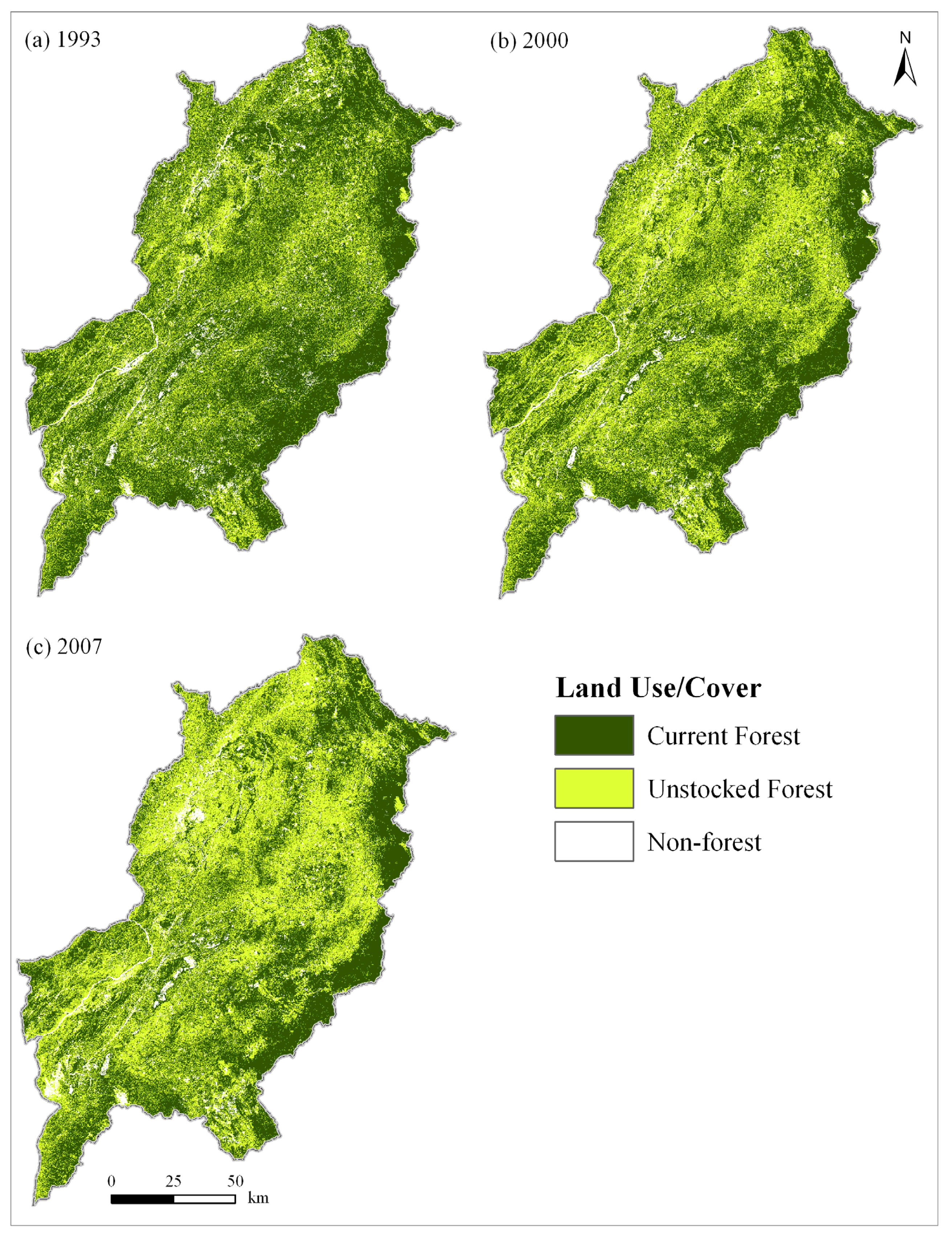
Biophysical (forest cover and GIS maps) and socioeconomic data were used to develop the model for simulating forest cover changes (Table 1). Forest cover maps (Figure 2 and Table 2) were produced from the classification of satellite imagery for 1993, 2000 and 2007 using a hybrid approach that combines unsupervised classification and decision trees [20]. Overall forest cover classification accuracy levels for the three dates range from 86% to 90%. The 1991–1992 and 2002 land use/cover maps produced by FIPD were used as reference data for assessing the accuraccy of the 1993 and 2000 forest cover maps. High resolution ALOS PRISM imagery (at 2.5 m spatial resolution) that was acquired in 2007 as well as secondary reference data, which were collected using handheld GPS devices during the 2009 fieldwork, were used for assessing the accuracy of the 2007 forest cover map. Biophysical and socioeconomic data such as roads, rivers, village (settlements) and number of people were obtained from the National Geographic Department (NGD) in Lao PDR, while elevation and slope were derived from SRTM (Shuttle Radar Topography Mission) data. Road, river and village (settlements) data were used to generate static driving factors such as “distance to major roads”, “distance to rivers” and “distance to town center” based on the euclidean distance procedures. Driving factors such as “distance to deforested areas” were defined as dynamic because these were generated and updated during model iteration [13]. Socioeconomic data such as the number of people in each household was used to produce population density data. Finally, all input datasets were resampled at 90 m × 90 m spatial resolution to match the spatial resolution of the SRTM digital elevation model (DEM).
3.2. Background—MCA Model
The MCA model combines the “weights of evidence” technique, Markov chains and a cellular automata (CA) model (Figure 3). The “weights of evidence” technique uses Bayes theorem of conditional probability to compute transition potential maps for each forest cover transition (e.g., current forest to unstocked forest) based on the statistical relationship between landscape determinants of forest cover change such as elevation and distance measures (Table 1). The “weights of evidence” technique was used in this study because it reduces the problems of bias and subjectivity, which are usually common in multicriteria evaluation techniques (MCE) [21]. In addition, previous studies have successfully used the “weights of evidence” technique for computing transition potential maps in tropical areas [8].
Markov chains are stochastic models that describe a process, which moves in a sequence of steps through a set of states [22]. In essence, the probability that the system will be in a given state at a given time (t2) is derived from the knowledge of its state at any earlier time (t1), and does not depend on the history of the system before time t1 [23]. Markov chains can be characterised as stationary or homogeneous in time if the transition probabilities depend only on the time interval t (that is, Δt = t2 − t1), and if the time period at which the process is examined is of no relevance [24,25]. We used the Markov chains in this study because the transition probabilities give the direction and magnitude of change that is useful for simulating forest cover changes [22]. Furthermore, the computation of the transition probabilities from land use/cover data is relatively easy since it is not computationally intensive.
Cellular automata (CA) models are bottom-up, individual-based dynamic models that were originally conceptualised by Ulam and Von Neumann in the 1940s in order to understand the behaviour of complex systems [26]. Generally, CA encompasses a space composed of a regular grid in one or two dimensions, a finite set of possible states associated with every cell (e.g., forest or non-forest), a neighbourhood composed of adjacent cells whose state influence the central cell, transition rules applied uniformly through time and space, and a discrete time at which the state of the system is updated [27-30]. Time progresses in discrete steps and all cells change their state simultaneously as a function of their own state, together with the state of the cells in their neighbourhood according to a specified set of transition rules [31].
Modelling approaches that integrate CA and Markov chains have long been explored [32,33]. A major advantage of the MCA approach is that biophysical and socioeconomic data can be integrated in order to parameterise the model [10]. Li and Reynolds [33] developed a hybrid Markov and CA model for simulating the effects of spatial pattern, drought, and grazing on the rates of rangeland degradation. Although their model was conceptually appealing, it did not account for the variations of transition probabilities over time. To overcome such limitations, Soares-Filho et al. [10] incorporated a saturation value parameter that is designed to vary transition rates through a dynamic feedback analysis of landscape changes. Their spatially explicit, multi-scale and dynamic stochastic CA modelling framework successfully simulated land use/cover changes in the Amazonian colonisation frontier [8,10]. Recently, the Dinamica EGO modelling framework has also introduced a scenario generator model that computes transition rates based on the integration of environmental and socioeconomic factors [13,34].
3.3. Model Calibration and Simulation Run
First, we used elevation, slope,“distance to major roads”, “distance to rivers”, “distance to town center”, “distance to deforested areas” and population density (Table 1) to compute transition potential maps based on the “weights of evidence” technique in Dinamica EGO [35-39]. In addition, the “weights of evidence” technique was used to quantify the influence of the driving factors (Table 1) on each type of forest cover transitions. In this study, “current forest to unstocked forest”, “current forest to non-forest”, “unstocked forest to current forest”, “unstocked forest to non-forest”, “non-forest to current forest”, and “non-forest to unstocked forest” transitions were considered for the computation of the transition potential maps. Since the basic assumption of the “weights of evidence” technique is that driving variables must be independent, we tested the correlation between the driving variables using the Crammer coefficient (V). Results indicated that elevation, “distance to major roads”, “distance to rivers”, “distance to town center”, “distance to deforested areas” and population density have values lower than the empirical threshold of 0.5 (V is less than 0.5) and thus are are not correlated [13,34]. Slope was not used in the final computation of the transition potential maps since it has a Crammer coefficient (V), which is more than 0.5 (Table 3).
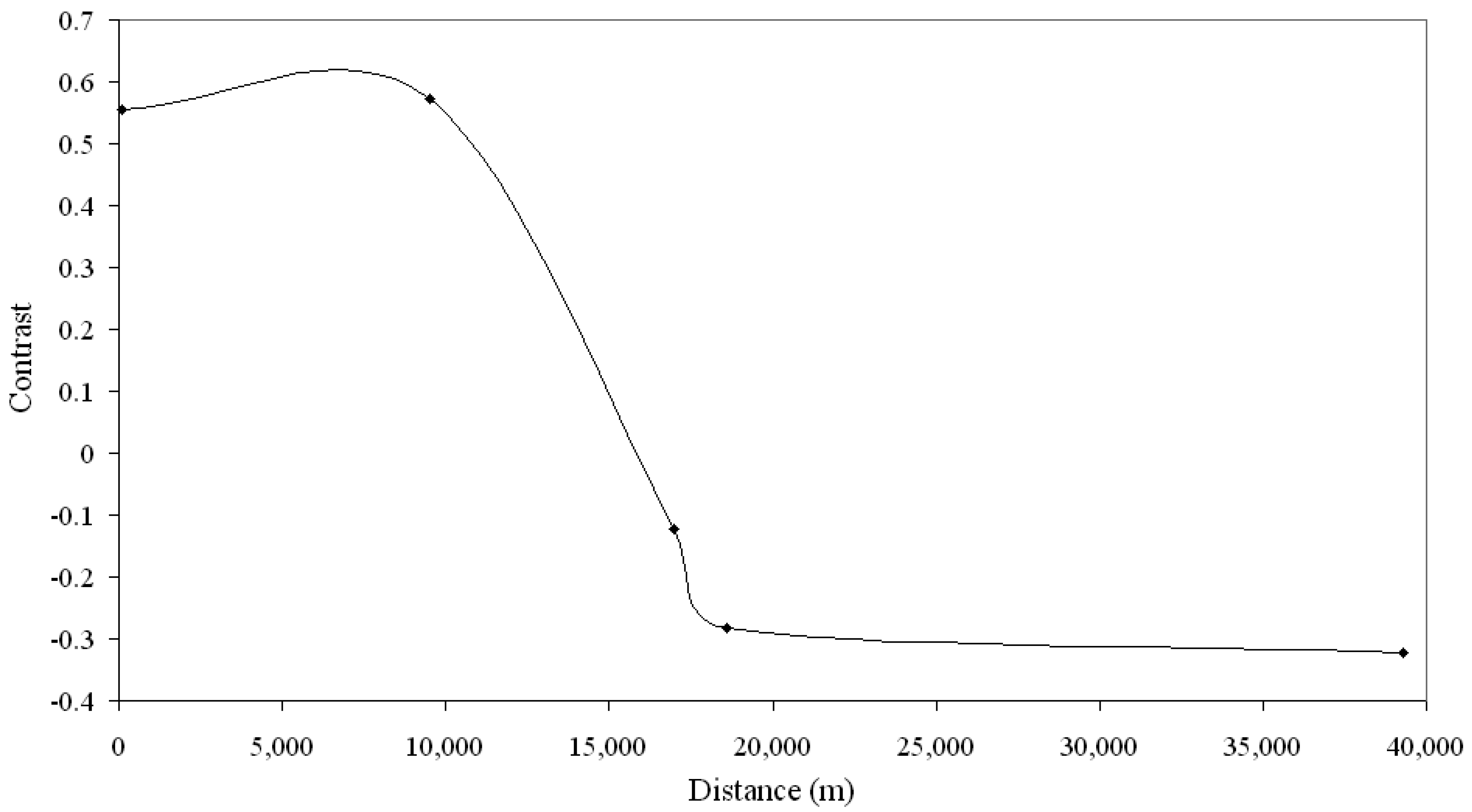
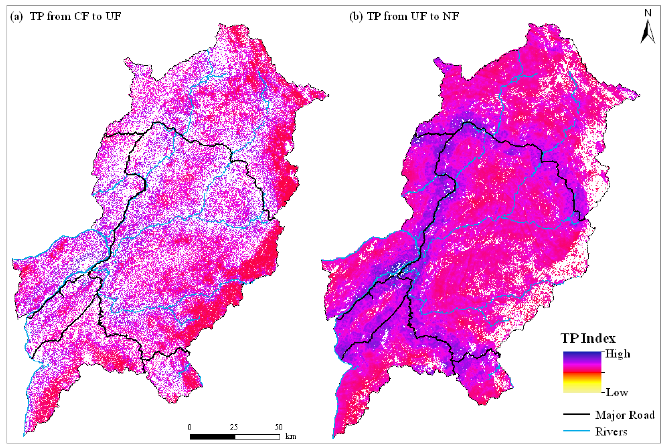
Spatial analysis of the “current forest to unstocked forest” and “unstocked forest to non-forest” transition potential maps revealed that high deforestation propensity is influenced by distance to major roads and rivers (Figure 4). This is consistent with the results from the “weights of evidence” analysis, which indicate that the decrease in current forest areas (that is, change from current forest to unstocked forest and non-forest) is largely influenced by distance to roads and rivers within 10,000 m buffer zones. Figure 5 shows contrast values, which indicate the relationship between “distance to major roads” and deforestation (that is, the change from current forest to unstocked forest). Contrast is the difference between the positive and negative weights (derived from the “weights of evidence” analysis) that is used to measure the correlation between a particular forest cover change and sampled training points for each variable [40]. Positive contrast values (above zero) indicate that areas within the 10,000 m distance ranges are more suscpetible to deforestation, while negative contrast values (below zero) show that areas over 10,000 m distance ranges are less susceptible to deforestation [35].
Following the computation of transition potential maps, we calculated transition probabilities for 1993–2000 and 2000–2007 using the Markov chains. Transition matrices were constructed from the cross tabulation of the 1993 to 2000 and 2000 to 2007 forest cover maps (Figure 2). The 1993–2000 transition probabilities were used as input in the MCA model, whereas the 2000–2007 transition probabilities were used to check the stationarity of the transition probabilities [23].
The following three datasets; (1) the initial forest cover map (1993), (2) the transition potential maps, and (3) the 1993–2000 transition probability matrix were used to simulate forest cover map up to 2007 based on the CA model functions available in Dinamica EGO. This CA model employs an expander transition function to expand or contract previous forest cover class patches, while the patcher transition function is used to form new patches [41]. The expander and patcher transition functions are composed of an allocation mechanism responsible for identifying cells with the highest transition probabilities for each transition [34,35]. For example, the expander transition function performs transitions from state i (current forest) to state j (unstocked forest) only in the neighbouring cells of state j in order to expand or contract forest cover class patches. The patcher function performs transitions from state i to state j only in the neighbouring cells with states other than j (e.g., non-forest) [34]. In order to simulate forest cover changes, both transition functions use a stochastic selecting mechanism [34,41]. First, the algorithm scans the initial forest cover map to sort out the cells with the highest probabilities and then arranges them in a data array [10,34]. After the initial step, cells are selected randomly from top to bottom of the data array. Finally, the forest cover map is again scanned to perform the selected transitions [10].
The sizes of new forest patches are set according to a lognormal probability function, whose parameters are defined by the mean patch size (MPS), patch size variance (VAR) and isometry (ISO) [34,35]. The parameters can be changed to produce various spatial patterns of forest cover changes. For example, an increase in mean patch size results in a less-fragmented landscape, while an increase in the patch size variance results in a more diverse landscape [34]. Isometry is a number that varies from 0 to 2 and thus, an isometry greater than one results in more isometric (equal) patches [34]. We calibrated the CA model by changing the internal parameters of the expander and patcher transition functions. The mean patch size and variance were computed from the original forest cover map using FRAGSTATS 3.3 [42], while the isometry was determined through trial and error (Table 4). The MCA model iterations were specified as 7, at an annual time step. This is because the MCA model iterations are specified according to the time difference between the initial forest cover map (1993) and the second forest cover map (2000). Finally, the model was set to run from 1993 (the initial year of simulation) to 2007, which is the year of the actual (observed) forest cover map. The simulated forest cover map (2007) was compared to the actual (observed) forest cover map (2007) in order to validate the accuracy of the model.
3.4. Scenario Modelling
Following calibration and validation, a scenario-driven MCA modelling approach was then used to simulate future forest cover changes under: (I) business-as-usual (BAU); (II) pessimistic; and (III) optimistic scenarios. We examined the total forest area (e.g., current forest and unstocked forest) under different conditions to simulate forest management scenarios for GHG emissions. Furthermore, a scenario-driven MCA modelling approach was employed because it provides a scientific basis to evaluate the consequences of different policy interventions, which can be used to support sustainable forestry management.
The BAU scenario assumed that historical forest cover changes observed between 1993 and 2000 under the current socioeconomic conditions would continue in the future. Thus, this scenario used annual transition probabilities between 1993 and 2000 as well as biophysical and socioeconomic factors such as elevation, “distance to major roads”, “distance to rivers”, “distance to town center”, “distance to deforested areas”, and population density in order to compute transition potential maps. For the pessimistic scenario, future forest cover changes were simulated under a scenario of increased infrastructure developments such as paved secondary roads and dam construction. Thus, we assumed that the current unpaved roads would have been upgraded to paved roads, while the proposed dams would have been constructed in the study area. Therefore, additional driving factors such as “distance to secondary paved roads” and reservoirs were included for computing transition potential maps under the pessimistic scenario. In addition, we modified the transition probability matrix between 1993 and 2000 in order to increase the deforestation rates. Consequently, the pessimistic scenario would induce a further reduction in current forest areas given the increased accessibility brought by infrastructure developments (e.g., secondary paved roads) as well as the modification of transition probabilities. Finally, for the optimistic scenario, future forest cover changes were simulated under strict enforcement of the forestry law and sustainable forest management policies (e.g., no deforestation in protected forest areas). Therefore, the protected forest area GIS coverage was used as a constraint to deforestation (for protecting current forest areas). In addition, the transition probability matrix (between 1993 and 2000) was modified by decreasing the transition probabilities from current forest to unstocked, and from current forest to non-forest. Table 5 shows the datasets for simulating the BAU, pessimistic and optimistic scenarios.
4. Results and Discussion
4.1. Analysis of Forest Cover Changes
Results show that current forest and unstocked forest areas were dominant in the study area (Figure 2). From 1993 to 2000, unstocked forest areas increased substantially from 5,975 km2 to 8,003 km2, while current forest areas decreased from 12,803 km2 to 10,987 km2. Generally, non-forest areas decreased slightly from 1,172 km2 to 961 km2. However, from 2000 to 2007, unstocked forest areas increased from 8,003 km2 to 9,043 km2, whereas current forest areas decreased from 10,987 km2 to 9,727 km2. In contrast to the 1993–2000 period, non-forest areas increased slightly from 961 km2 to 1,181 km2 between 2000 and 2007.
Table 6 shows that “current forest to unstocked forest”, “non-forest to unstocked forest”, “unstocked forest to non-forest” and “current forest to non-forest” were the major forest cover changes in Luangprabang province between 1993 and 2000. The high rate of “current forest to unstocked forest” changes compared to the low rate of “unstocked to current forest” changes between 1993 and 2000 indicate significant loss of current forest areas. However, the “unstocked forest to non-forest” changes were less than the “non-forest to unstocked forest” changes, which shows that substantial regrowth of 260 km2 occurred in the study area. This is partly attributed to the regrowth of unstocked forest during the shifting cultivation cycle, whereby abandoned agriculture fields are left to recover soil fertility.
The major forest cover changes between 2000 and 2007 were “current forest to unstocked forest”, “unstocked forest to current forest”, “non-forest to unstocked forest”, “unstocked forest to non-forest” and “current forest to non-forest” (Table 6). While the “current forest to unstocked forest” changes increased during the 2000–2007 period, “unstocked forest to current forest” changes also increased substantially compared to the 1993–2000 period. Consequently, the 2000–2007 period was characterised by lower “current forest to unstocked forest” changes given the high forest regrowth (unstocked forest to current forest changes was 1,159 km2). In general, forest cover change analyses revealed high rate of “current forest to unstocked forest” changes between 1993 and 2000 and lower rate of “current forest to unstocked forest” changes between 2000 and 2007.
4.2. Analysis of Transition Probabilities
Table 7 shows the forest cover transition probabilities between 1993 and 2000, calculated on the basis of the frequency distribution of the observations. The transition probabilites were computed from forest cover maps (which have a spatial resolution of 90 m). The diagonal of the transition probability matrix represents the self-replacement probabilities, that is the probability of a forest cover class remaining the same (shown in bold in table 7), whereas the off-diagonal values indicate the probability of a change occurring from one forest cover class to another. The self-replacement probabilities for the current forest and unstocked forest classes were above 50%, while the self-replacement probability for non-forest class was low (30%) (Tables 7). The transition probability from current forest to unstocked forest was 13%, whereas the transition probability from unstocked forest to current was 1%, which implies continued loss of current forest areas in the future. In contrast, the transition probability from current forest to non-forest was low (2%). However, the transition probability from non-forest to current forest increased to 5%, which suggest low regrowth in the future. It is interesting to note that the transition probability from unstocked forest to non-forest was low (5%), whereas the transition probability from non-forest to unstocked forest was high (66%). This implies that there will be substantial regrowth of the unstocked forest in the future.
It should be noted that key Markov chain assumptions such as independence and stationarity (homogeneity) were not tested in this study. However, the comparison of the 1993–2000 (Table 7) and 2000–2007 (Table 8) transition matrices suggests that the transition probabilities were not stationary. To minimise this limitation, we employed a multi-step Markov chain analysis available in Dinamica EGO that incorporates a saturation value parameter, which varies the transition probabilities through a dynamic feedback analysis of landscape changes [10,35].
4.3. Model Validation
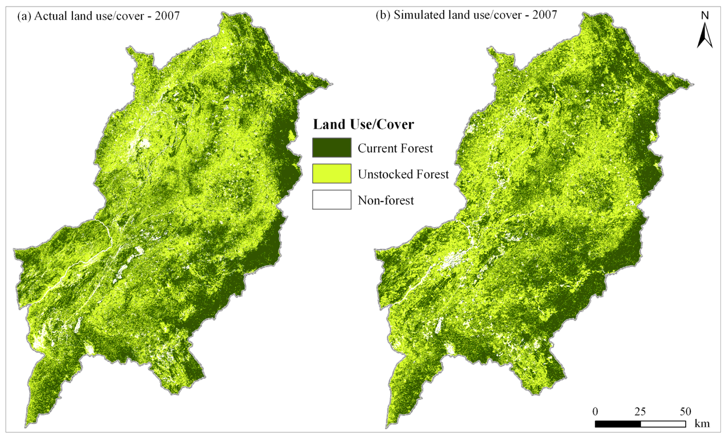
For model validation, we used the conventional Kappa statistic to compare the simulated forest cover maps for 2007 with the actual (observed) satellite-derived forest cover map for 2007 under the BAU scenario. Visual analysis of the simulated forest cover map in 2007 revealed that the MCA model simulated the current forest and unstocked forest areas relatively well (Figure 6). The best agreement is shown in the unstocked forest and current forest classes (Figure 7). For example, the actual unstocked forest class was 9,043 km2, while the corresponding simulated class was 9,194 km2. On the other hand, the current forest class was 9,727 km2, while the corresponding simulated class was 9,841 km2. The results indicate that forest cover classes such as current forest and unstocked forest areas, which occupies the highest proportion of area in the province have higher accuracy. This suggests that the model's simulation accuracy increases with the proportion of a given forest cover class. While the nonforest class was slightly underpredicted (the actual class was 1,180 km2 compared to the corresponding simulated class, which was 914 km2), the MCA's overall simulation accuracy was 0.8, which is relatively good for simulating future forest cover changes. The MCA model accuracy is within the range of accuracies observed in other studies that have used similar spatial simulation modelling approaches [41,43-45].
Although we did not validate the accuracy of the model in terms of location, visual analysis revealed that location was relatively underpredicted, particularly for the non-forest class (Figure 6). However, it should be noted that the major focus of this study was on simulating the quantity of forest cover changes since it would be used for setting REDD/REDD+ reference scenarios. Therefore, accuracy of the current and unstocked forest areas in terms of quantity is important. It also noteworthy that precise information concerning the location of carbon dioxide emissions is not required for setting reference scenarios because global warming effects are derived from the total carbon dioxide concentrations in the atmosphere, not the carbon dioxide's precise location of origin [11,46].
4.4. Simulated Future Forest Cover Changes under Different Scenarios
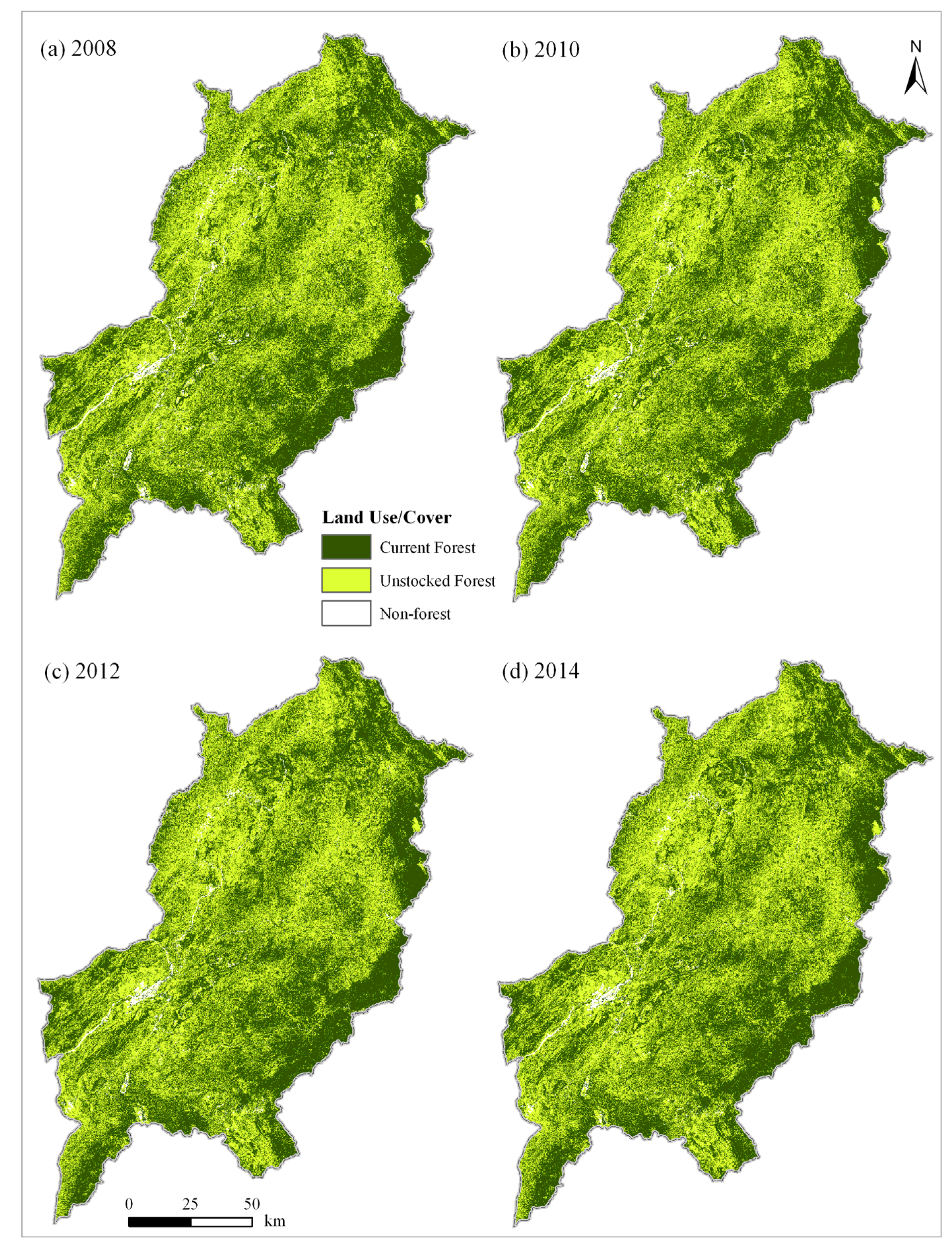
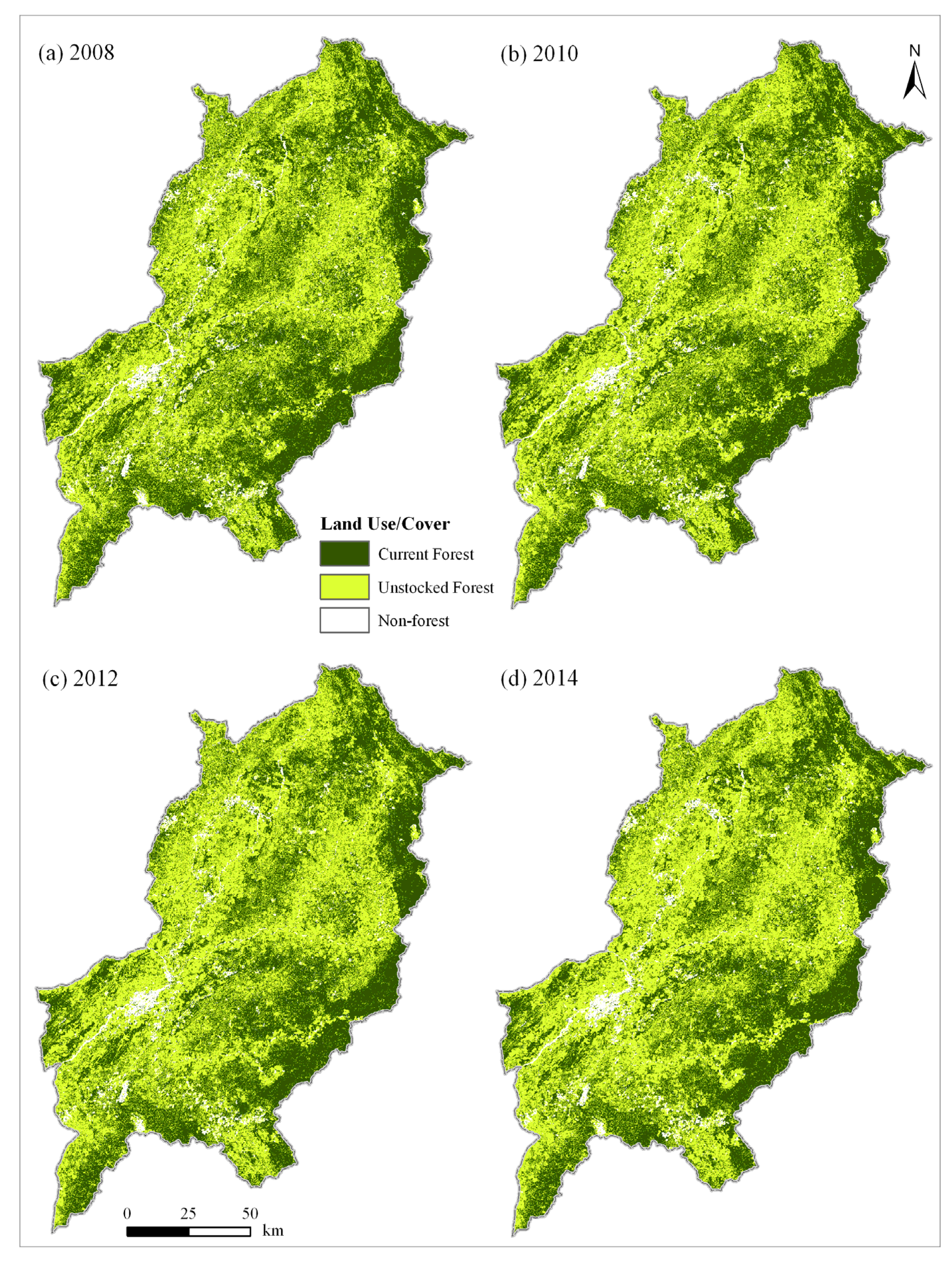
Based on the calibration and validation of the MCA model (for 2007), we simulated future forest cover changes up to 2014 under the BAU, pessimistic and optimistic scenarios. The final models were run twenty times for each scenario [41]. Under the BAU scenario, the MCA model simulations projected that current forest areas would decrease from 9,727 km2 in 2007 to 8,811 km2 in 2014, while unstocked forest areas would increase substantially from 9,043 km2 to 10,279 km2 over the same period (Figure 8). In addition, non-forest areas would decrease from 1,181 km2 in 2007 to 860 km2 in 2014 (Figure 8). Taking into consideration the increasing population [15], the simulated forest cover changes indicate increasing pressure on forest resources in Luangprabang province, which potentially threatens rural livelihoods. Generally, future “current forest to unstocked forest” changes under the BAU scenario would be mainly concentrated near Luangprabang city as well as along the major roads and rivers where the majority of people live. Under the pessimistic scenario, the MCA model simulations projected that current forest areas would decrease significantly from 9,727 km2 in 2007 to 6,851 km2 in 2014, while unstocked forest areas would increase significantly from 9,043 km2 to 10,164 km2 over the same period (Figure 9). In addition, non-forest areas would increase substantially from 1,181 km2 in 2007 to 2,939 km2 in 2014 (Figure 9). The rapid decline in current forest areas on one hand and the increase in unstocked forest and non-forest areas on the other hand imply rapid “current forest to unstocked forest” changes in the future. It is important to note that “current forest to unstocked forest” changes would also be concentrated near Luangprabang city as well as along the major and secondary paved roads, and rivers. While the pessimistic scenario considered additional data such as “distance to secondary paved roads”, the simulated future forest cover changes are quite conservative because they do not consider both legal and illegal forest logging directly in the model.
Under the optimistic scenario, the MCA model simulations projected an increase in current forest areas (from 9,727 km2 in 2007 to 11,112 km2 in 2014), while unstocked forest areas would also decrease moderately from 9,043 km2 to 8,542 km2 over the same period (Figure 10). However, non-forest areas would decrease significantly from 1,181 km2 in 2007 to 297 km2 in 2014 (Figure 10). The MCA forest cover change simulations revealed an increase in current forest areas in the future since the protected forest areas were used as a constraint to deforestation.
Results from the forest cover change scenarios reflect the significance of assumptions adopted under the business-as-usual (BAU), pessimistic and optimistic scenarios. For example, under the BAU scenario, current forest areas would decline gradually in the future, while under the pessimistic scenario, current forest areas would decline rapidly. However, such declines in current forest areas would not occur if forestry laws that protect and conserve the protected forest areas under the optimistic scenario are strictly enforced.
5. Summary and Conclusions
Taking Luangprabang province as a case study, the objective of this study was to simulate future forest cover changes under the BAU, pessimistic and optimistic scenarios. The initial forest cover map (1993), the “1993 to 2000” transition probabilities and the transition potential maps were used to simulate forest cover changes up to 2007. The simulated forest cover map (2007) was compared to the actual forest cover map (2007) in order to test the accuracy of the Markov-cellular automata (MCA) model. Visual and statistical analyses revealed that current forest and unstocked forest classes were relatively well simulated, while the non-forest class was slightly underpredicted. The model's overall simulation accuraccy was 0.8.
Following the successful calibration of the MCA model, future forest cover changes were simulated (up to 2014) under the BAU, pessimistic and optimistic scenarios. The MCA simulations under BAU scenario indicated that the current forest cover change trends such as the decrease in current forest areas and the increase in unstocked forest areas would continue to persist in the study area. Furthermore, the MCA simulations under the pessimistic scenario revealed a rapid decrease in current forest areas and substantial increases in unstocked forest areas, which implies severe loss of forest areas in the future. Since forest resources provide life-sustaining products such as food, medicines and fuelwood, the BAU and pessimistic scenarios are important because they indicate plausible future forest cover changes in the study area. Nevertheless, the optimistic scenario projected that current forest areas would increase if strict forestry laws enforcing conservation of protected forest areas are implemented.
Spatial simulation modelling approaches based on the MCA model are critical because simulated future forest cover changes under the BAU can be combined with forest carbon stock in order to set reference emission scenarios. Therefore, this study constitutes an important contribution to the REDD/REDD+ implementation framework since reference scenarios can be used to establish a benchmark, which will provide the basis for giving REDD/REDD+ incentives [11]. The MCA model applied in Luangprabang province has several strengths. First, the model's transition potential maps are calibrated with a set of biophysical and socioeconomic driving variables under different scenarios. Consequently, the simulated future forest cover changes under different simulation scenarios provide important insights, which can be used by decision makers for REDD/REDD+ preparedness activities. For example, the different simulation scenarios can be used to identify regional-scale patterns of forest cover changes, which would be used to target areas that require immediate intervention. Second, government policy (particularly, the use of the protected areas as a constraint to deforestation) was incorporated in the MCA model under the optimistic scenario. Third, the MCA model's calibration and validation functions permits the comparison of the simulated and observed forest cover changes, and thus allow for the improvement of the model. The initial forest cover map (1993), the transition potential maps and the 1993–2000 transition probabilities were used to calibrate the model and perform simulations up to 2007 using CA-based expander and patcher functions. Then, the simulated forest cover map for 2007 was compared to the observed (actual) forest cover map for 2007. In essence, the MCA model has clearly separated the data (1993 forest cover map, transition potential maps and 1993–2000 transition probabilites) used for calibrating the model and the data (2007 forest cover map) used for validating the model [47].
While the MCA model has demonstrated that it is possible to simulate future forest cover changes in Luangprabang province, there are certain limitations that should be noted. First, location (e.g., non-forest class) is underpredicted because the MCA model emphasises linear forest cover changes, while in the real world non-linear forest cover changes occur. Another reason is that the MCA model assumed that biophysical factors such roads remained constant given the lack of updated road data in the study area. Second, for calibrating and running the MCA model in an area that experiences dynamic land use and forest cover changes (due to shifting cultivation and other agricultural activities as well as the impact of both legal and illegal logging), more forest cover data is required in order to capture the temporal heterogeneity. Finally, it should be noted that the raster-based MCA model applied in the study area is sensitive to different cell resolution and neighbourhood configurations [26]. Therefore, future studies should improve the capacity of the MCA model by including more temporal forest cover maps (at an interval of two to three years) and more GIS data that correspond to the forest cover change maps. Furthermore, novel geographic object-based CA models should be incorporated in the MCA modelling framework in order to minimise problems related to scale and neighbourhood sensitivity [26].


| Data | Input data |
|---|---|
| Biophysical | Forest cover maps (1993 and 2000) |
| DEM (elevation and slope) | |
| Distance to major roads | |
| Distance to rivers | |
| Distance to town center | |
| Distance to deforested areas | |
| Socioeconomic | Population density |
| Forest cover class | Description |
|---|---|
| Current forest | Includes natural and plantation forest areas with crown density more than 20% and an area equal to or greater than 0.5 ha. Trees should reach a minimum height of 5 m. |
| Unstocked forest | Previously forested areas in which crown density has been reduced to less than 20% due to disturbances (e.g., shifting cultivation or logging). |
| Non-forest | Cropland, ray, grassland, settlement areas, roads, barren land, rocks, rivers and reservoirs. |
| A | B | C | D | E | F | G | |
|---|---|---|---|---|---|---|---|
| A | 1 | ||||||
| B | 0.034 | 1 | |||||
| C | 0.038 | 0.998 | 1 | ||||
| D | 0.050 | 0.999 | 0.344 | 1 | |||
| E | 0.012 | 0.002 | 0.025 | 0.057 | 1 | ||
| F | 0.049 | 0.008 | 0.097 | 0.049 | 0.025 | 1 | |
| G | 0.013 | 0.016 | 0.165 | 0.055 | 0.085 | 0.047 | 1 |
Note: A: elevation; B: slope; C: distance to main roads; D: distance to rivers; E: distance to town center; F: distance to deforested areas; G: population density.
| MPS | VAR | ISO | |
|---|---|---|---|
| Current forest | 15 | 30 | 1.0 |
| Unstocked forest | 9 | 20 | 0.5 |
| Non-forest | 3 | 5 | 0.1 |
Note: MPS: mean patch size; VAR: variance; ISO: isometry.
| Data | Input data | BAUS | PS | OS |
|---|---|---|---|---|
| Biophysical | Forest cover maps (1993 and 2000) | * | * | * |
| Elevation | * | * | * | |
| Distance to major roads | * | * | * | |
| Distance to secondary paved roads | * | |||
| Distance to rivers | * | * | * | |
| Distance to town center | * | * | * | |
| Distance to deforested areas | * | * | ||
| Reservoirs | * | |||
| Protected forest areas | * | |||
| Socioeconomic | Population density | * | * | * |
Note: BAUS: business-as-usual scenario; PS: pessimistic scenario; OS: optimistic scenario.*Indicates input data considered under each scenario.
| Forest cover class | 1993–2000 | 2000–2007 |
|---|---|---|
| Current forest to unstocked forest | 1,619 | 2,179 |
| Current forest to non-forest | 299 | 277 |
| Unstocked forest to current forest | 48 | 1,159 |
| Unstocked forest to non-forest | 313 | 573 |
| Non-forest to current forest | 54 | 37 |
| Non-forest to unstocked forest | 768 | 593 |
| 2000 | ||||
|---|---|---|---|---|
| Current forest | Unstocked forest | Non-forest | ||
| 1993 | Current forest | 0.85 | 0.13 | 0.02 |
| Unstocked forest | 0.01 | 0.94 | 0.05 | |
| Non-forest | 0.05 | 0.65 | 0.30 | |
| 2007 | ||||
|---|---|---|---|---|
| Current forest | Unstocked forest | Non-forest | ||
| 2000 | Current forest | 0.78 | 0.19 | 0.03 |
| Unstocked forest | 0.15 | 0.78 | 0.07 | |
| Non-forest | 0.04 | 0.62 | 0.34 | |
Acknowledgments
This study was supported by a grant from the Forestry Agency under the Ministry of Agriculture, Forestry and Fisheries (MAFF), Japan. We thank the Forestry Inventory and Planning Division (FIPD) in Lao PDR and other stakeholders for their assistance during the course of the study. We are grateful for the useful comments and suggestions from Rajesh Bahadur Thapa from the University of Tsukuba in Japan. Finally, we thank the anonymous reviewers for their thorough critique of the manuscript drafts.
References and Notes
- De Gryze, S. Cashing in carbon credits: Can GIS cost-effectively measure forest gains. Geoworld 2009, 22, 25–27. [Google Scholar]
- Climate Change 2007: Synthesis Report; Intergovernmental Panel on Climate Change (IPCC): Geneva, Switzerland, 2007. Available online: http://www.ipcc.ch/ (accessed on 3 August 2009).
- Sustainable Forest Management and Conservation of Tropical Rainforests; FAO: Rome, Italy, 1995.
- Realising REDD+: National Strategy and Policy Options; Angelsen, A., Brockhaus, M., Kanninen, M., Sills, E., Sunderlin, W.D., Wertz-Kanounnikoff, S., Eds.; CIFOR: Bogor, Indonesia, 2009.
- Angelsen, A. REDD models and baselines. Int. For. Rev. 2008, 10, 465–475. [Google Scholar]
- Terrestrial Carbon Group. How to Include Terrestrial Carbon in Developing Nations in the Overall Climate Change Solution, The Terrestrial Carbon Group's Policy Paper. 2008. Available online: http://www.terrestrialcarbon.org/site/DefaultSite/filesystem/documents/Terrestrial%20 Carbon%20Group%20080808.pdf (accessed on 14 January 2011).
- Brown, S.; Hall, M.; Andrasko, K.; Ruiz, F.; Marzoli, W.; Guerrero, G.; Masera, O.; Dushku, A.; De Jong, B.; Cornell, J. Baselines for land-use change in the tropics: Application to avoided deforestation projects. Mitigat. Adaptat. Strateg. Glob. Change 2007, 12, 1001–1026. [Google Scholar]
- Soares-Filho, B.S.; Nepsta, D.C.; Curran, L.M.; Cerqueira, G.C.; Garcia, R.A.; Ramos, C.A.; Voll, E.; McDonald, A.; Lefebvre, P.; Schlesinger, P. Modelling conservation in the Amazon basin. Nature 2006, 23, 520–523. [Google Scholar]
- Sciotti, R. Demographic and ecological factors in FAO tropical deforestation modelling. In World Forests from Deforestation to Transition; Palo, M., Vanhanen, H., Eds.; Kluwer Academic Publishing: Dordrecht, The Netherlands, 2000. [Google Scholar]
- Soares-Filho, B.S.; Alencar, A.; Nepstads, D.; Cerqueira, G.; Diaz, M.C.V.; Rivero, S.; Solorzanos, L.; Voll, E. Simulating the response of land-cover changes to road paving and governance along a major Amazonian highway: The SANTAREM-Cuiaba corridor. Glob. Change Biol. 2004, 10, 745–764. [Google Scholar]
- GOFC-GOLD 2009. A Source Book of Methods and Procedures for Monitoring and Reporting Anthropogenic Greenhouse Gas Emissions and Removals Caused by Deforestation, Gains and Losses of Carbon stocks in Forests Remaining Forests, and Forestations; GOFC-GOLD Report version COP15–1; GOFC-GOLD, Natural Resources Canada: Edmonton, Alberta, Canada, 2009. [Google Scholar]
- Veldkamp, T.; Lambin, E.F. Predicting land-use change. Agr. Ecosyst. Environ. 2001, 85, 1–6. [Google Scholar]
- Teixerira, A.M.G.; Soares-Filho, B.S.; Freitas, S.R.; Metger, J.P. Modeling landscape dynamics in an Atlantic rainforest region: Implications for conservation. Forest Ecol. Man. 2009, 257, 1219–1230. [Google Scholar]
- Messina, J.; Walsh, S. 2.5 D morphogenesis: Modeling landuse and landcover dynamics in the Ecuadorian Amazon. Plant Ecol. 2001, 156, 75–88. [Google Scholar]
- Wada, Y.; Rajan, K.S.; Shibasaki, R. Modeling the spatial distribution of shifting cultivation in Luangprabang, Lao PDR. Environ. Plan. B Plan. Design 2007, 34, 261–278. [Google Scholar]
- Walsh, S.J.; Entwisle, B.; Rindfuss, R.R.; Page, P.H. Spatial simulation modelling of land use/land cover change scenarios in northeastern Thailand: A cellular automata approach. J. Land Use Sci. 2006, 1, 5–28. [Google Scholar]
- Lambin, E.F.; Turner, B.L.; Geist, H.J.; Agbola, S.B.; Angelsen, A.; Bruce, J.W.; Coomes, O.T.; Dirzo, R.; Fischer, G.; Folke, C.; et al. The causes of land-use and land-cover change: Moving beyond the myths. Glob. Environ. change 2001, 11, 261–269. [Google Scholar]
- Lao Department of Statistics. Lao PDR Statistical Year Book-2008; Department of Statistics: Vientiane, Lao PRD, 2009. [Google Scholar]
- FAO. Forest Resource Assessment 2005. Country Report- Lao PDR; WP 182; FAO: Rome, Italy, 2005. [Google Scholar]
- Asia Air Survey. Progress Report on the Study on the Strengthening of Methodological and Technological Approaches for Reducing Deforestation and Forest Degradation within the REDD Implementation Framework: Application in Lao PDR; Asia Air Survey: Shin Yurigaoka, Japan, 2010. [Google Scholar]
- Hosseinali, F.; Alesheikh, A.A. Weighting spatial information in GIS for copper mining exploration. Am. J. Appl. Sci. 2008, 5, 1187–1198. [Google Scholar]
- Weng, Q. Land use change analysis in the Zhujiang Delta of China using satellite remote sensing, GIS and stochastic modelling. J. Environ. Manage. 2002, 64, 273–284. [Google Scholar]
- Petit, C.; Scudder, T.; Lambin, E. Quantifying processes of land-cover change by remote sensing: Resettlement and rapid land-cover changes in south-eastern Zambia. Int. J. Rem. Sens. 2001, 22, 3435–3456. [Google Scholar]
- Karlin, S.; Taylor, H.M. A First Course in Stochastic Processes; Academic Press: New York, NY, USA, 1975; p. 557. [Google Scholar]
- Lambin, E.F. Modelling Deforestation Processes: A Review; Office for Official Publications of the European Community: New York, NY, USA, 1994; p. 128. [Google Scholar]
- Moreno, N.; Wang, F.; Marceau, D.J. A geographic object-based approach in cellular automata modeling. Photogramm. Eng. Rem. Sens. 2010, 76, 183–191. [Google Scholar]
- Tobler, W. Cellular geography. In Philosophy in Geography; Gale, S., Olsson, G., Eds.; D. Reidel Publishing Company: Dordrecht, The Netherlands, 1979; pp. 379–386. [Google Scholar]
- Couclelis, H. Cellular worlds: A framework for modeling micro-macro dynamics. Environ. Plan. A 1985, 17, 585–596. [Google Scholar]
- Engelen, G.; White, R.; Uljee, I.; Drazan, P. Using cellular automata for integrated modeling of socio-environmental systems. Environ. Monit. Assess 1995, 34, 203–214. [Google Scholar]
- Wolfram, S. Cellular automata as models of complexity. Nature 1984, 311, 419–424. [Google Scholar]
- White, R.; Engelen, G. Cellular automata as the basis of integrated dynamic regional modeling. Environ. Plan. B 1997, 24, 235–246. [Google Scholar]
- Zhou, G.; Liebhold, A.M. Forecasting the spread of gypsy moth outbreaks using cellular transition models. Landsc. Ecol. 1995, 10, 177–186. [Google Scholar]
- Li, H.; Reynolds, J.F. Modeling effects of spatial pattern, drought, and grazing on rates of rangeland degradation: A combined Markov and cellular automaton approach. In Scale in Remote Sensing and GIS; Quattrochi, D.A., Goodchild, M.F., Eds.; Lewis Publishers: Boca Raton, FL, USA, 1997; pp. 211–230. [Google Scholar]
- Almeida, C.M.; Batty, M.; Monteiro, A.M.V.; Camara, G.; Soares-Filho, B.S.; Cerqueira, G.C.; Pennachin, C.L. Stochastic cellular automata modelling of urban land use dynamics: Empirical development and estimation. Comput. Environ. Urban Syst. 2003, 27, 481–509. [Google Scholar]
- UFMG (Universidade Federal de Minas Gerais). Dinamica EGO; Centro de Sensoriamento Remoto/Universidade Federal de Minas Gerais: Belo Horizonte, Brazil, 2009. Available online: http://www.csr.ufmg.br/dinamica/ (accessed on 6 April 2010).
- Almeida, C.M.; Monteiro, A.M.V.; Camara, G.; Soares-Filho, B.S.; Cerqueira, G.C.; Pennachin, C.L.; Batty, M. GIS and remote sensing as tools for the simulation of urban land-use change. Int. J. Rem. Sens. 2005, 26, 759–774. [Google Scholar]
- Agterberg, F.P.; Cheng, Q. Conditional independence test for weights-of-evidence modeling. Natur. Resour. Res. 2002, 11, 249–255. [Google Scholar]
- Soares-Filho, B.S.; Assuncao, R.M.; Pantuzzo, A. Modeling the spatial transition probabilities of landscape dynamics in an Amazonian colonization frontier. BioScience 2001, 51, 1039–1046. [Google Scholar]
- Bonham-Carter, G.F.; Agterberg, F.P.; Wright, D.F. Integration of geological data sets for gold exploration in Nova Scotia. Photogram. Eng Remote. Sens. 1988, 54, 1585–1592. [Google Scholar]
- Ford, A.; Clarke, K.C.; Raines, G. Modeling settlement patterns of the late classic Maya civilization with Bayesian methods and geographic information systems. Ann. Assn. Amer. Geogr. 2009, 93, 496–520. [Google Scholar]
- Soares-Filho, B.S.; Cerqueira, G.C.; Pennachin, C.L. DINAMICA—A stochastic cellular automata model designed to simulate the landscape dynamics in an Amazonian colonization frontier. Ecol. Model. 2002, 154, 217–235. [Google Scholar]
- McGarigal, K.; Cushman, S.A.; Neel, M.C.; Ene, E. FRAGSTATS: Spatial Pattern Analysis Program for Categorical Maps; University of Massachusetts: Massachusetts, MA,USA, 2002. [Google Scholar]
- Paegelow, M.; Olmedo, M.T.C. Possibilities and limits of prospective GIS land cover modelling—A compared case study: Garrotxes (France) and Alta Alpujarra Granadina (Spain). Int. J. Geogr. Inform. Sci. 2005, 19, 697–722. [Google Scholar]
- Myint, S.W.; Wang, L. Multicriteria decision approach for land use land cover change using Markov chain analysis and a cellular automata approach. Can. J. Rem. Sens. 2006, 32, 390–404. [Google Scholar]
- Kamusoko, C.; Aniya, M.; Bongo, A.; Munyaradzi, M. Rural sustainability under threat in Zimbabwe—Simulation of future land use/cover changes in the Bindura district based on the Markov-cellular automata model. Appl. Geogr. 2009, 29, 435–447. [Google Scholar]
- Pontius, R.G., Jr.; Walker, R.; Yao-Kumah, R.; Arima, E.; Aldrich, S.; Caldas, M.; Vergara, D. Accuracy assessment for a simulation model of Amazonian deforestation. Ann. Assn Amer. Geogr. 2007, 97, 677–695. [Google Scholar]
- Verburg, P.H.; Schot, P.P.; Dijst, M.J.; Veldkamp, A. Land use change modelling: Current practice and research priorities. Geojournal 2004, 61, 309–324. [Google Scholar]
© 2011 by the authors; licensee MDPI, Basel, Switzerland. This article is an open access article distributed under the terms and conditions of the Creative Commons Attribution license (http://creativecommons.org/licenses/by/3.0/).
Share and Cite
Kamusoko, C.; Oono, K.; Nakazawa, A.; Wada, Y.; Nakada, R.; Hosokawa, T.; Tomimura, S.; Furuya, T.; Iwata, A.; Moriike, H.; et al. Spatial Simulation Modelling of Future Forest Cover Change Scenarios in Luangprabang Province, Lao PDR. Forests 2011, 2, 707-729. https://doi.org/10.3390/f2030707
Kamusoko C, Oono K, Nakazawa A, Wada Y, Nakada R, Hosokawa T, Tomimura S, Furuya T, Iwata A, Moriike H, et al. Spatial Simulation Modelling of Future Forest Cover Change Scenarios in Luangprabang Province, Lao PDR. Forests. 2011; 2(3):707-729. https://doi.org/10.3390/f2030707
Chicago/Turabian StyleKamusoko, Courage, Katsumata Oono, Akihiro Nakazawa, Yukio Wada, Ryuji Nakada, Takahiro Hosokawa, Shunsuke Tomimura, Toru Furuya, Akitaka Iwata, Hiromichi Moriike, and et al. 2011. "Spatial Simulation Modelling of Future Forest Cover Change Scenarios in Luangprabang Province, Lao PDR" Forests 2, no. 3: 707-729. https://doi.org/10.3390/f2030707