Estimating the Aboveground Biomass of Robinia pseudoacacia Based on UAV LiDAR Data

Abstract

Robinia pseudoacacia is widely planted in the Loess Plateau as a major soil and water conservation tree species because of its dense canopy, complex structure, and strong soil and water conservation ability. The precise measurement of small-scale locust forest biomass is crucial to monitoring and evaluating the carbon sequestration functions of soil and water conservation vegetation. This study focuses on an artificial locust forest planted in the early 1990s in Caijiachuan Basin, Jixian County, Shanxi Province. A drone equipped with LiDAR was used to obtain point cloud data and generate a canopy height model. A watershed segmentation algorithm was used to identify tree vertices and extract individual trees. A relationship model between tree height, diameter at breast height, and biomass, combined with sample survey data, was established to explore the spatial distribution of biomass in the artificial locust forest at the level of the entire basin. The results show the following: (1) the structural parameters of locust extracted using UAV point cloud data have a good degree of fit and accuracy, and the recall rate is 72.7%; (2) the average error rate of the extracted maximum tree height value of locust is 7%, that of the minimum tree height value is 14%, and that of the average tree height value is 18%; (3) the average error rate of the extracted maximum diameter at breast height of locust is 15%, that of the minimum diameter at breast height is 37%, and that of the average diameter at breast height is 36%; and (4) the average error rate of the biomass estimation of locust calculated using point cloud data is 16.0%.

1. Introduction

A forest’s aboveground biomass is the energy basis and material source for its ecosystem’s ecological service function [1]. It is a key indicator used to evaluate forest health and the sustainable utilization of vegetation resources [2]. It is also the basis for the study of ecosystem carbon cycles and carbon storage [3]. The accurate biomass monitoring of small-scale soil and water conservation forests is key to scientifically assessing their ecological service functions, such as soil conservation [4], water conservation [5], diversity conservation [6], and soil improvement [7], as well as laying the groundwork for a scientific response to climate change and to achieving carbon neutrality and carbon peaks [3].

The traditional method of aboveground biomass estimation is mainly based on field surveys and biomass regression models, which are constructed by counting tree height, diameter at breast height, and other related parameters of individual trees in sample plots through anisotropic growth equations [8]. These biomass measurements can be used as basic data for the macro-estimation of biomass in the whole study area [9]. However, determining biomass by measuring forest structural parameters is costly and labor-intensive [10].

Estimating aboveground biomass using remote sensing is mainly based on features such as spectrum, index, and texture, which are extracted from optical remote sensing images to establish biomass inversion models [11,12,13]. Although these models can reach high levels of accuracy, they are not usually generalizable and are limited by the accuracy of image resolution. They also make it difficult to achieve biomass estimation at the individual tree scale [14]. Microwave remote sensing data can also be used to obtain stand factors such as tree height and crown width; combined with allometric growth models, these data can aid in the construction of a biomass estimation model [15,16]. However, microwave radars are easily influenced by the environment and monitored targets, among other limitations on large-scale biomass estimation [17].

A laser radar uses a pulsed laser to measure a range or the distance to the Earth‘s surface [18]. A sensor measures the return time of the laser pulse and can then be calibrated using the Global Positioning System (GPS) to provide absolute x, y, and z values for each return pulse [19]. In the context of forest biomass estimation, the first recorded signal is reflected from the highest surface of the forest, and the final return signal is usually considered to be reflected from its lowest point. At present, UAV LiDAR is not only widely used in the biomass estimation of Betula platyphylla [20], Populus davidiana [21], Picea crassifolia [22], Pinus sylvestris var.mongolica [23], Larix gmelinii [24], and other tree species but also of coniferous forests [25,26,27], the Greater Khingan Range [28,29], cities [30], tropical forests [31], and other large areas. Thus far, UAV LiDAR has found success in extracting individual trees in the case of species whose crowns are essentially conical, like those mentioned above. However, given that Robinia pseudoacacia has a relatively flat crown, more robust research is needed on estimating its aboveground biomass using UAV LiDAR.

Therefore, our research object was an artificial locust forest planted in the early 1990s in Caijiachuan River Basin, Jixian County, Shanxi Province. The relationship between the growth data of locust and the point cloud data obtained using UAV was established by combining the point cloud data with the tree height, DBH, and aboveground biomass data obtained using plot surveys. The aim was to provide an effective UAV LiDAR-based method for estimating the biomass of the locust forest on the level of the entire basin and to then provide data supporting the evaluation of the carbon sink capacity of soil and water conservation forests.

2. Materials and Methods

2.1. Study Area

The study area is located in the Caijiachuan River Basin, home to the National Field Scientific Observation and Research Station for Forest Ecosystems in Jixian County, Shanxi Province. The geographical coordinates are 110°39′45″–110°47′45″ E, 36°14′27″–36°18′23″ N. The terrain is high in the east and low in the west, with an area of 39.33 km² and a basin length of about 14 km. The elevation is 900–1513 m. The annual average temperature is 10.2 °C, and the annual average precipitation is 575.9 mm. Rainfall is mainly concentrated from July to September, accounting for about 59.5% of the annual precipitation. The area has a warm temperate continental climate. The brown soils that predominate in the area are of a Loess parent material and are slightly alkaline. The Caijiachuan River Basin has abundant plant resources, with 194 species of common woody plants, 180 herbaceous plants, and 141 traditional Chinese herbs. Since the 1970s, afforestation has been carried out in the basin, producing a forest coverage rate of over 80%. The upstream mainly consists of natural secondary forests, populated by species such as Populus davidiana and Quercus mongolica; the middle reaches are mainly artificial forests composed of Robinia pseudoacacia and Pinus tabuliformis; and the lower reaches are wasteland and farmland. Apple (Malus pumila), pear (Pyrus spp.), apricot (Armeniaca vulgaris), and other fruit trees are planted in the slope terraced fields. The area of the Caijiachuan River Basin selected for this study, which was planted with acacia forests in the 1990s (Figure 1), has an area of 2.06 km².

2.2. Data Sources and Processing

2.2.1. Sample Survey

From May to August 2022, 14 quadrats (

Table 1. Basic information on the sample area.

Plot ID	Longitude	Latitude	Density (Tree/hm2)	Altitude/m	Aspect/°	Slope/°	Tree Height/m (avg. ± SD)	CV	AGB/kg
1	110°44′49.4810″ E	36°16′28.2848″ N	950	1181	335	25	11.46 ± 2.63	Middle	2107.996
2	110°45′27.1682″ E	36°16′15.3416″ N	1156	1112	65	27	10.17 ± 3.59	High	1117.346
3	110°44′24.8988″ E	36°16′32.1703″ N	1150	1166	180	20	10.34 ± 3.39	High	3134.514
4	110°45′26.5978″ E	36°16′18.8931″ N	1475	1119	75	26	10.77 ± 3.53	High	2386.459
5	110°45′50.7713″ E	36°16′30.3138″ N	1500	1117	60	15	8.27 ± 3.91	High	2344.06
6	110°44′31.3110″ E	36°16′30.0838″ N	1525	1149	225	23	8.03 ± 2.31	Middle	3978.908
7	110°46′11.1767″ E	36°16′18.0881″ N	1950	1022	70	31	10.1 ± 2.61	Middle	4275.538
8	110°46′08.4736″ E	36°16′18.0780″ N	2200	958	50	15	10.15 ± 2.34	Middle	3177.047
9	110°45′53.9493″ E	36°16′29.8737″ N	2050	1086	40	15	9.56 ± 2.54	Middle	1734.486
10	110°45′52.9134″ E	36°16′32.7558″ N	2444	1088	35	0	10.2 ± 2.19	Middle	2331.556
11	110°44′32.5029″ E	36°16′42.0954″ N	2475	1168	196	22	12.98 ± 3.03	Middle	3383.656
12	110°45′19.9705″ E	36°16′52.4691″ N	2475	1110	195	28	12.05 ± 3.63	Middle	3156.846
13	110°45′41.4187″ E	36°16′20.3522″ N	3022	1056	150	14	8.85 ± 2.85	High	2108.085
14	110°45′44.2842″ E	36°16′22.4456″ N	3300	1081	180	36	9.05 ± 2.68	Middle	3355.007

) 20 m × 20 m in size were selected in the study area to measure each tree, and indexes such as diameter, tree height, and crown width were recorded. Diameter at breast height was measured using a caliper, tree height was measured using a telescopic rod, and crown width was measured using a tape measure. Standard trees were selected based on the average tree height and average diameter at breast height of each plot. The mathematical equation between tree height, diameter at breast height, and biomass was fitted based on standard tree data and used to estimate the total biomass of each locust plot.

2.2.2. LiDAR Data Acquisition and Processing

From May to June 2023, a DJI M300RTK UAV equipped with a Zen L1 radar lens was used for data acquisition. The ground mode was used; the flight speed was 10 m/s, the flight height was 80 m, the laser side overlap rate was 80%, and the average point density was 147 points/m². A total of 43.4 GB of LiDAR data and 2046 UAV images covering the study area were obtained.

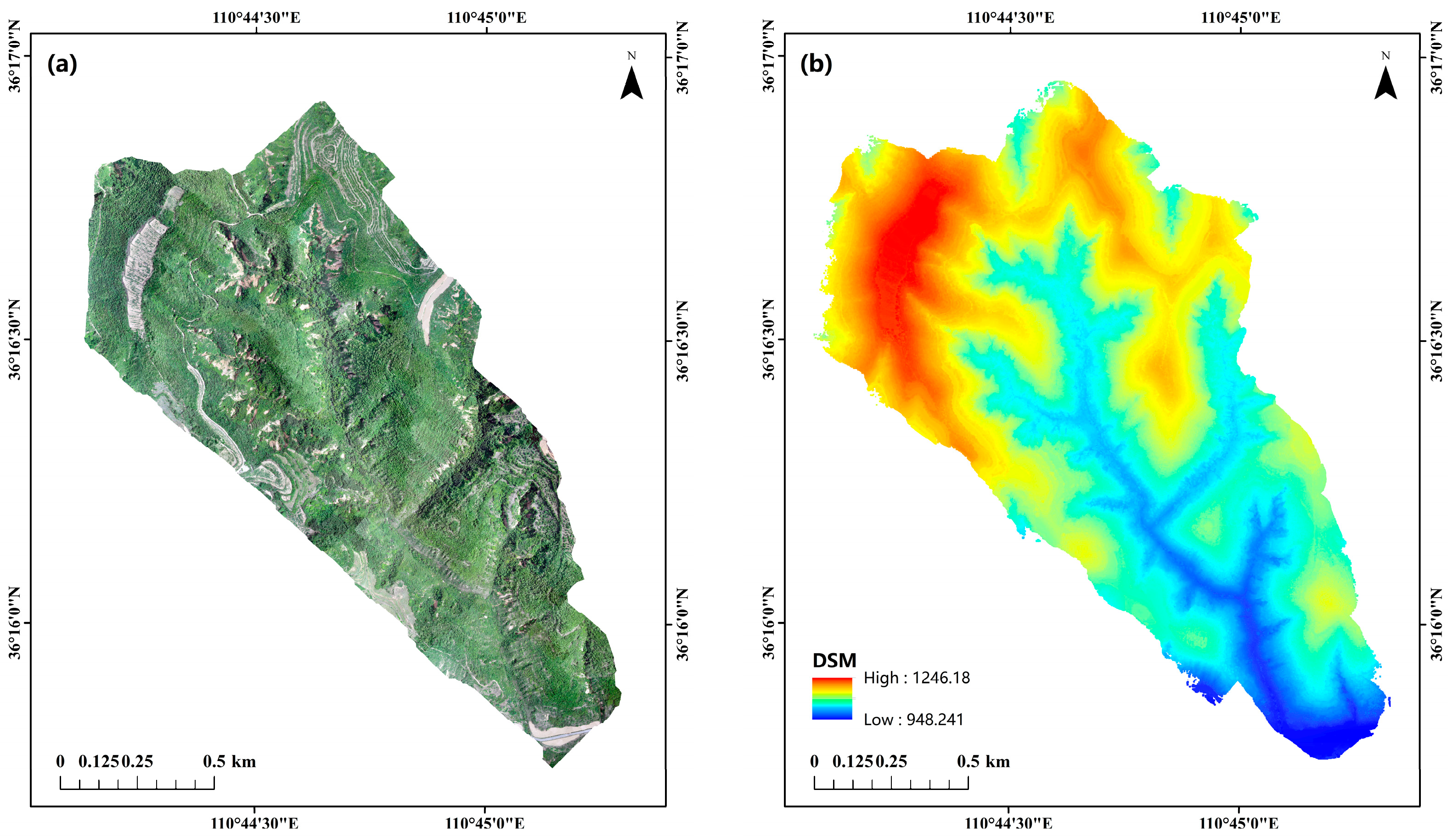
We used DJI Maps (v3.6) software to generate an orthographic UAV image of the study area (Figure 2a); the spatial resolution was 1 m. The progressive encryption triangulation filtering algorithm was used to classify the ground point cloud and the surface point cloud [32,33]. The co-Kriging interpolation method was used to generate the digital surface model (Figure 2b) and the digital elevation model (Figure 2c). The difference between the digital surface model and the digital elevation model was calculated to obtain the canopy height model (Figure 2d) of the study area, with a spatial resolution of 0.5 m.

2.2.3. Split Window Size

Segmentation windows of 0.1 m × 0.1 m, 0.2 m × 0.2 m, 0.3 m × 0.3 m, 0.4 m × 0.4 m, and 0.5 m × 0.5 m were selected. The variable window-filtering algorithm was used to analyze the optimal segmentation window for individual tree extraction [34].

2.2.4. Individual Tree Extraction and Segmentation

Firstly, individual tree position detection was carried out and the spatial position of the crown vertex was determined. Secondly, the extracted crown vertices were used as seed points to perform individual tree crown segmentation. During tree vertex recognition, a local maximum algorithm was used, and raster data were searched through the moving window step by step to determine whether the center point of the search window was the local maximum value [35]. If that was the case, the pixel was marked as the tree vertex, and then the watershed segmentation algorithm was used to accurately segment the individual tree crown by using the optimal segmentation window [36,37]. This was achieved using the point cloud toolbox in MATLAB R2023b. The results of individual tree vertex recognition and individual tree extraction are shown in Figure 3 and Figure 4.

2.2.5. Verification of Individual Tree Segmentation Results

The UAV orthophoto map was used as the verification base map to evaluate the individual tree segmentation results, which were classified as either correct segmentation, missed segmentation, or over-segmentation. Recall and accuracy rates were used to evaluate the interpretation results [38].

$$r=\frac{T_p}{T_p+F_n}$$

(1)

$$p=\frac{T_p}{T_p+F_p}$$

(2)

In the above formula, r represents the recall rate, that is, the proportion of the number of correctly segmented plants to the number of actually investigated plants; p represents the correct rate, that is, the proportion of the number of correctly segmented plants to the number of plants extracted from point cloud data; T_p represents the number of correctly segmented plants; F_n represents the number of missing segmentation plants, that is, single trees that were not detected by the point cloud data; F_p represents the number of over-segmented trees, that is, instances in which the point cloud data divided a tree into multiple trees.

Taking the sample data as the measured value and the point cloud data extraction value as the estimated value, the tree height, diameter, and biomass error rates of the point cloud data were calculated.

$$e=\frac{\left(\left|E-M\right|\right)}{M}\times 100\%$$

(3)

In the above formula, e represents the error rate; E represents the estimated value; and M represents the measured value.

3. Results

3.1. Height–Diameter–Biomass Models

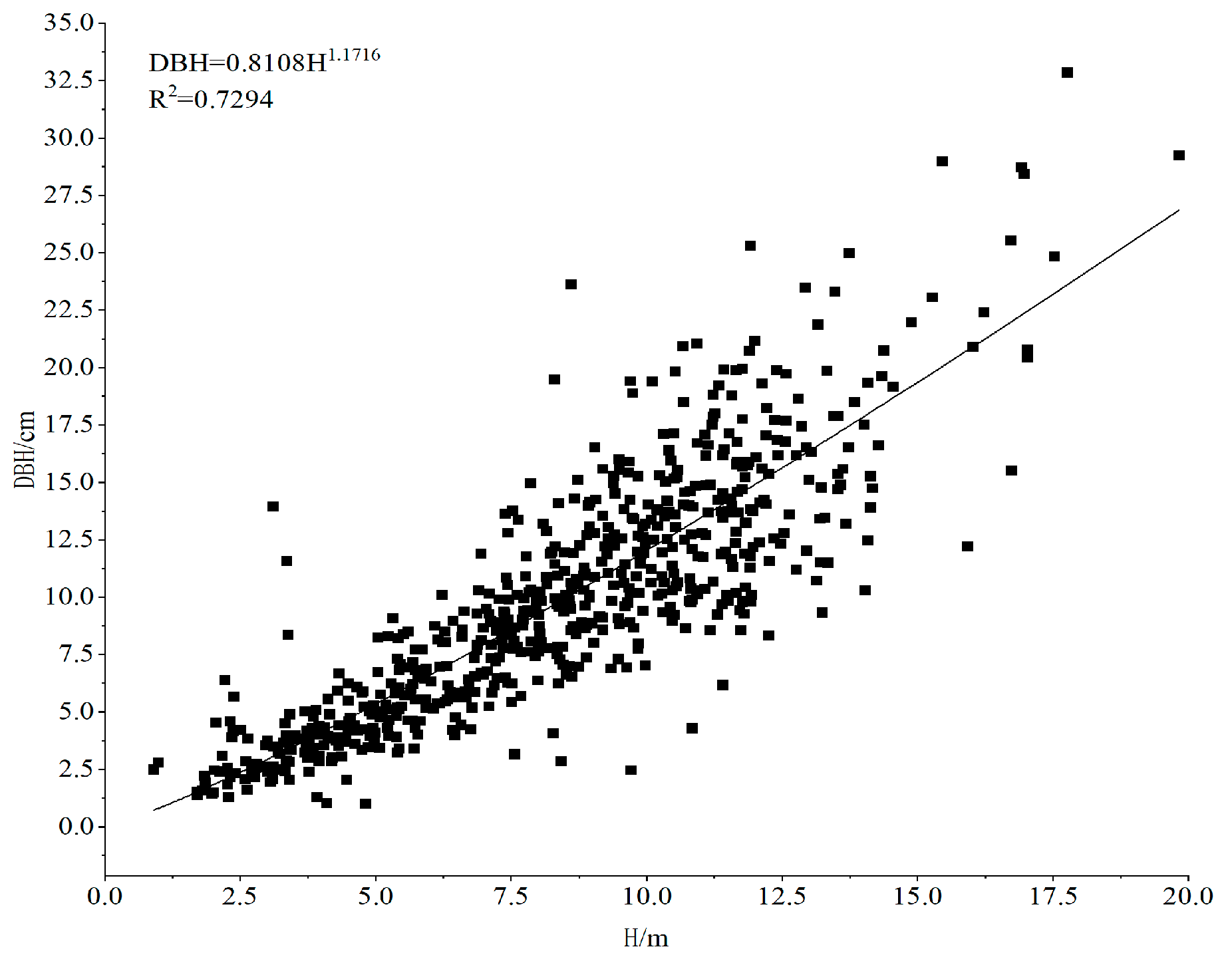
The relationship between the tree height and diameter of 514 individual locust trees in the study area, based on the data obtained from the ground quadrat survey, is shown in Figure 5. The regression equation of tree height and diameter was obtained by regression fitting with nonlinear function:

$$DBH=0.8108 \times H^{1.1716}$$

(4)

In the above formula, DBH is the diameter at breast height, and the unit is cm; H is the tree height, and the unit is m; and the correlation coefficient R² = 0.7294.

The height, diameter at breast height, and biomass of 14 standard trees were measured. The mathematical relationship between tree height, diameter at breast height, and biomass was fitted, and the fitting results are shown in

Table 2. Nonlinear biomass estimation models of Robinia pseudoacacia.

Estimation Models	Fitting Formula	R2	MAE	RMSE
AGB = aDBHb	AGB = 3.362 × DBH1.11	0.67	12.086	8.398
AGB = aHb	AGB = 3.438 × H1.07	0.41	12.086	11.34
AGB = a(DBH2 H)b	AGB = 2.111 × (DBH2 H)0.4333	0.70	4.514	8.188
AGB = aDBHb Hc	AGB = 2.354 × DBH0.9392 H0.3171	0.69	11.595	8.595
AGB = a(DBH3/H) b	AGB = 6.24 × (DBH3/H)0.4261	0.58	13.454	9.481

. The best fitting relationship was selected from Table 2.

Based on a comprehensive comparison of the R², MAE, and RMSE produced by the five models, the optimal aboveground biomass model was selected and is as follows:

$$AGB=2.111 \times {\left({DBH}^{2}H\right)}^{0.4333}$$

(5)

In the above formula, AGB is the aboveground biomass of a single plant, and the unit is kg; DBH is the diameter at breast height, and the unit is cm; and H is the tree height, and the unit is m.

Using the above diameter–height regression equation, the diameter of individual trees segmented by point cloud data was calculated, and then the aboveground biomass of locust in the study area was estimated using the height–diameter–biomass model.

3.2. Analysis of Segmentation Window Size and Individual Tree Recognition Accuracy

Table 3. The results of extracting the number of individual trees of Robinia pseudoacacia with different segmentation windows.

Plot ID	2	3	4	5	6	7	8	9	10	13	14	SUM
Reality	60	31	44	32	63	52	22	49	34	64	63	514
0.1 × 0.1 m	47	33	28	28	50	52	22	44	42	58	70	476
Tp	39	25	14	22	46	40	20	37	32	52	47	374
Fn	21	6	30	10	17	12	2	12	2	12	16	132
Fp	8	8	14	6	4	12	2	7	10	6	23	102
r/%	75.0	80.6	31.8	68.8	73.0	76.9	90.9	75.5	94.1	81.3	74.6	72.7
p/%	83.0	75.8	50.0	78.6	92.0	75.5	90.9	82.2	76.2	89.7	67.1	78.6
0.2 × 0.2 m	40	32	25	30	45	46	21	40	38	54	64	435
Tp	32	24	11	24	41	33	19	32	28	48	41	333
Fn	28	7	33	8	22	19	3	17	6	16	22	173
Fp	8	8	14	6	4	13	2	8	10	6	23	102
r/%	61.5	77.4	25.0	75.0	65.1	63.5	86.4	65.3	82.4	75.0	65.1	64.7
p/%	80.0	75.0	44.0	80.0	91.1	71.7	90.5	80.0	73.7	88.9	64.1	76.6
0.3 × 0.3 m	35	27	19	25	37	42	19	36	31	45	43	359
Tp	27	19	5	19	33	29	17	28	21	39	20	257
Fn	33	12	39	13	30	23	5	21	13	25	43	249
Fp	8	8	14	6	4	13	2	8	10	6	23	102
r/%	51.9	61.3	11.4	59.4	52.4	55.8	77.3	57.1	61.8	60.9	31.7	50.0
p/%	77.1	70.4	26.3	76.0	89.2	69.0	89.5	77.8	67.7	86.7	46.5	71.6
0.4 × 0.4 m	32	23	18	22	29	36	15	31	22	38	30	296
Tp	24	15	4	16	29	26	13	23	21	33	24	228
Fn	36	16	40	16	34	26	9	26	13	31	39	278
Fp	8	8	14	6	0	10	2	8	1	5	6	68
r/%	46.2	48.4	9.1	50.0	46.0	50.0	59.1	46.9	61.8	51.6	38.1	44.3
p/%	75.0	65.2	22.2	72.7	100.0	72.2	86.7	74.2	95.5	86.8	80.0	77.0
0.5 × 0.5 m	25	15	17	20	25	30	12	28	20	31	24	247
Tp	18	10	4	14	23	20	10	21	18	25	19	182
Fn	42	21	40	18	40	32	12	28	16	39	44	324
Fp	7	5	13	6	2	10	2	7	2	6	5	65
r/%	34.6	32.3	9.1	43.8	36.5	38.5	42.5	42.9	52.9	39.1	30.2	35.4
p/%	72.0	66.7	23.5	70.0	92.0	66.7	83.3	75.0	90.0	80.6	79.2	73.7

Data points 1, 11, 12 are damaged.

presents the results of individual tree segmentation conducted using 0.1 m × 0.1 m, 0.2 m × 0.2 m, 0.3 m × 0.3 m, 0.4 m × 0.4 m, and 0.5 m × 0.5 m segmentation windows. It is evident that there were a total of 514 locust trees in the measured quadrats. The recall and accuracy rates of the segmentation were calculated according to Formulas (1) and (2). It can be seen that when the segmentation window is 0.1 m × 0.1 m, the highest recall rate of individual tree segmentation is 72.7%, and the correct rate is 78.6%. This result is similar to the result of single tree extraction obtained by Yin et al. [33]. The total number of individual tree extractions obtained using the 0.1 m × 0.1 m segmentation window is 476, the number of correct segmentations is 374, and the recall rate is 72.7%. On the other hand, the minimum recall rate of the 0.5 m × 0.5 m segmentation window is 36%, and there are more instances of missing segmentation.

Eleven plots were used to verify the results of individual tree segmentation (Figure 6). It can be seen that the greater the number of locust trees, the more likely it is for values to be underestimated.

3.3. Results and Analysis of Extracted Tree Height

Figure 7 depicts the estimated tree height of each quadrat based on point cloud data and the corresponding measured tree height. It can be seen that the estimated height of locust is between 6.38 m and 15.58 m. According to Formula (3), the average error rate of the maximum tree height was 7%, that of the minimum tree height was 14%, and that of the average tree height was 18%.

Figure 8 represents a comparison between the estimated and measured maximum and average tree height. Within the range of 10–16 m, the maximum tree height of eight out of the eleven sample plots was overestimated; in two plots, the estimated maximum tree height was the same as the measured value, and in one plot, it was lower than the measured value. Within the range of 8–11 m, the average tree height values of ten plots were overestimated, and they were underestimated for only one sample plot.

3.4. Results and Analysis of Extracted DBH

Figure 9 represents the estimated DBH of each quadrat based on point cloud data and the corresponding measured DBH. It can be seen that the DBH of locust was between 5.28 cm and 27.42 cm. According to Formula (3), the average error rate of the maximum diameter at breast height was 15%, that of the minimum diameter at breast height was 37%, and that of the average diameter at breast height was 36%.

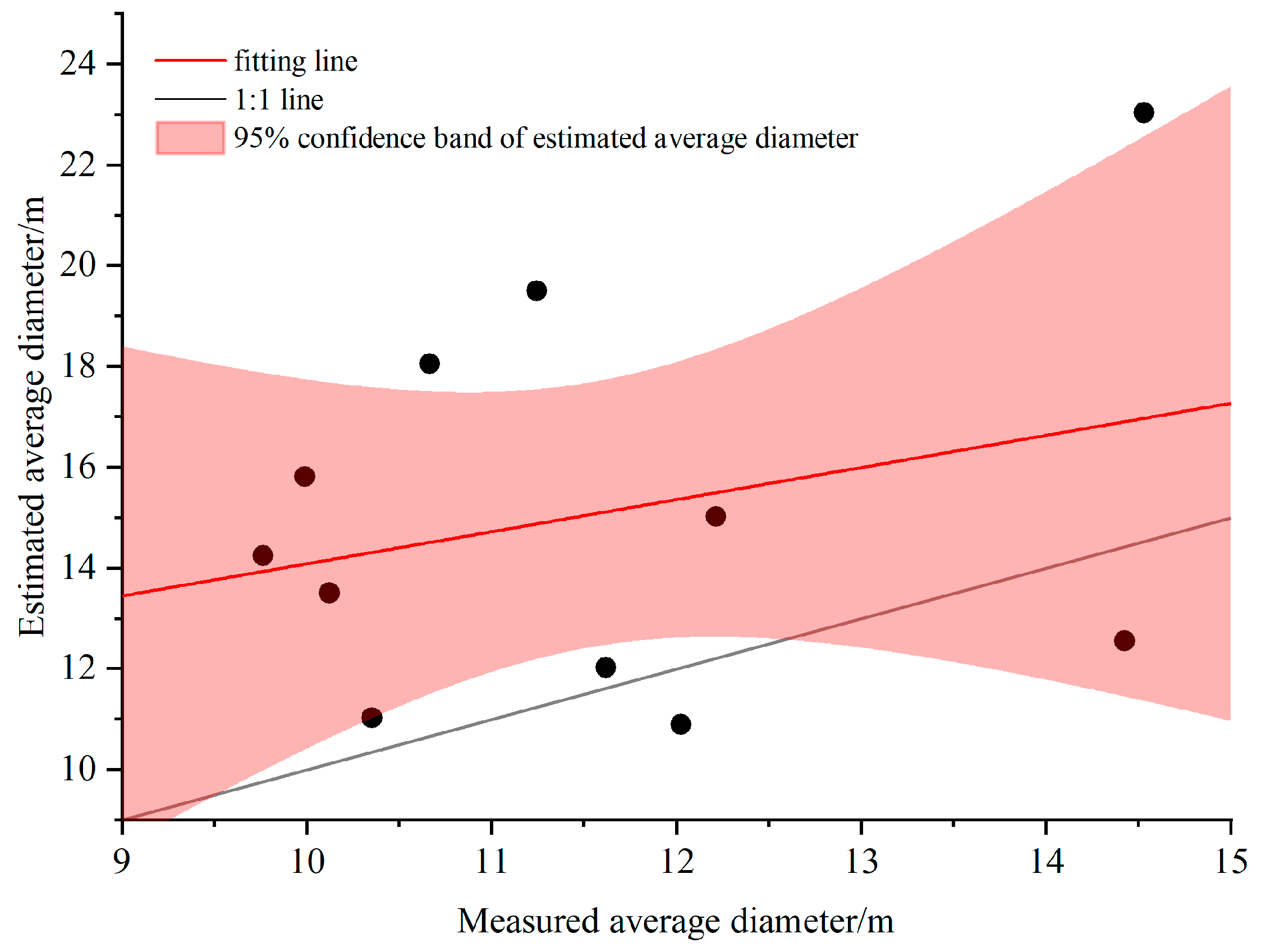
Figure 10 compares the extracted and measured values of the average diameter at breast height. It can be seen that in nine plots, the estimated average diameter was overestimated, while in two plots, it was underestimated.

3.5. Estimation and Analysis of Biomass

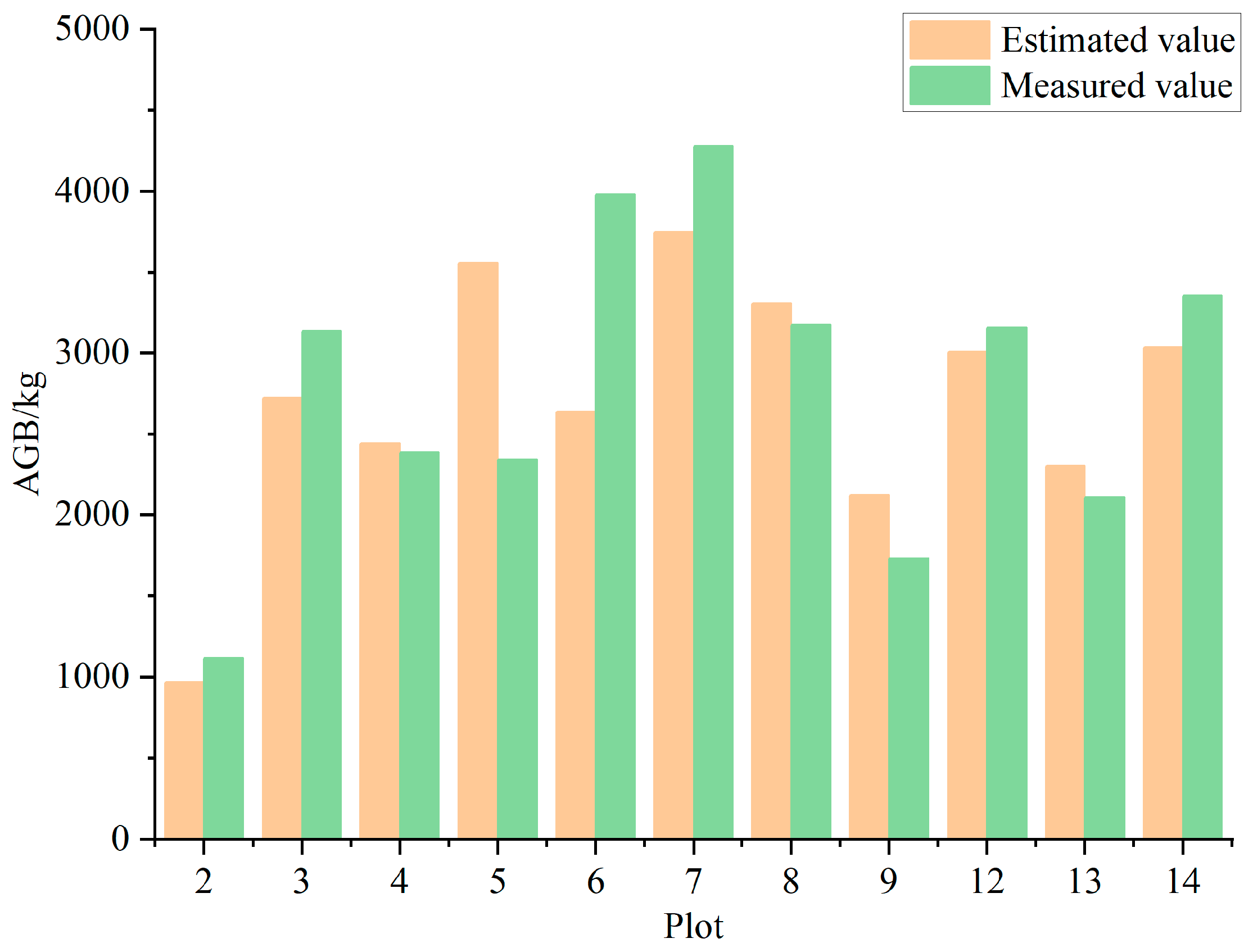
Biomass was estimated using Formulas (4) and (5). Figure 11 represents the estimated biomass value of each quadrat based on point cloud data and the corresponding measured biomass value. According to Formula (3), the average error rate of the estimated biomass value was 16%.

Figure 12 depicts a comparison between measured and estimated biomass, showing that point cloud data can be used to estimate the biomass of locust.

3.6. Biomass Estimation and Analysis in the Study Area

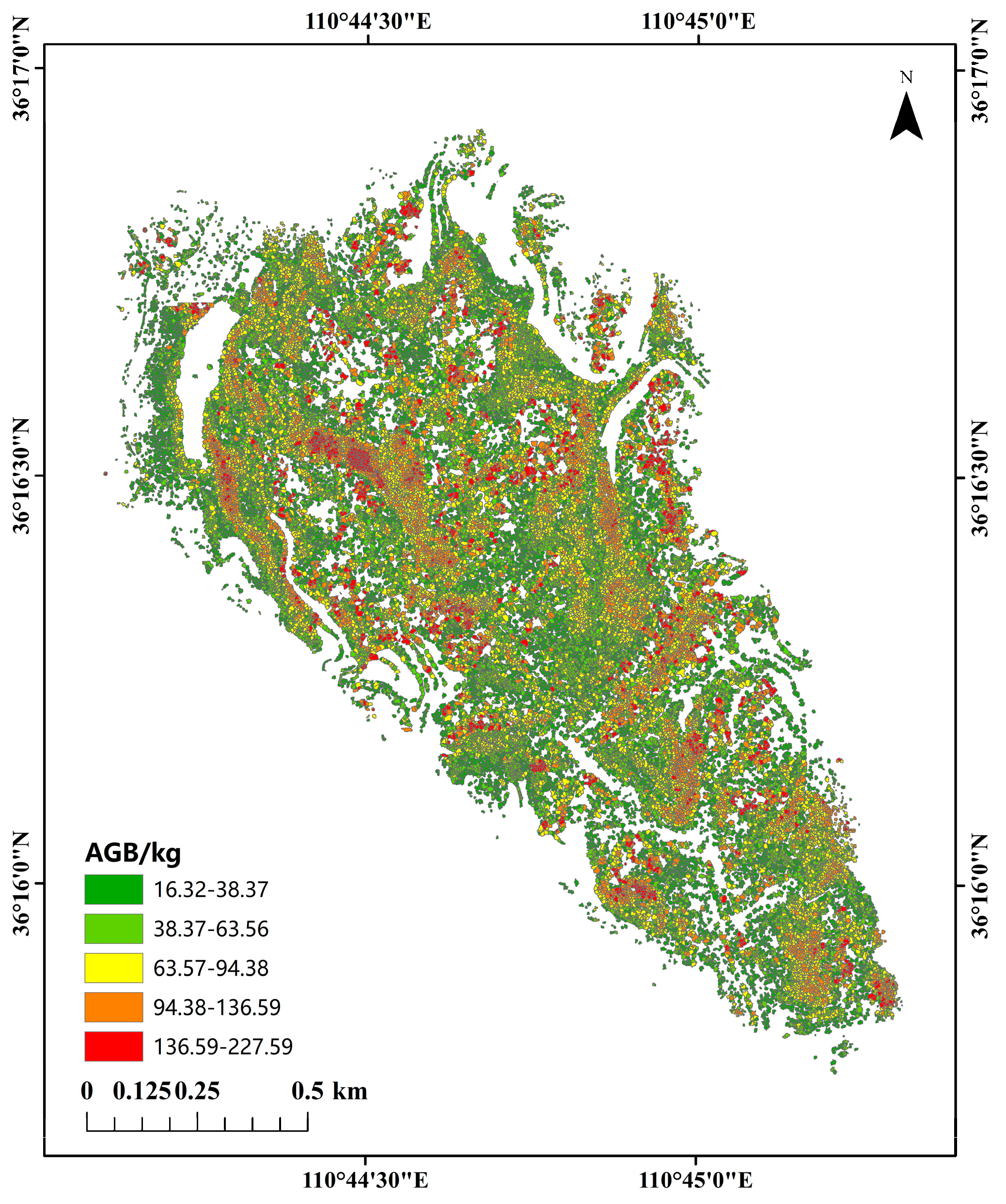
Figure 13 maps the spatial distribution of the aboveground biomass of single locust trees in the study area, which ranges from 16.32 kg to 227.59 kg, with an average of 56.38 kg.

The global Moran’s I index was used to further analyze the spatial aggregation degree of locust aboveground biomass distribution in the study area. The Moran’s I index was 0.338, the significance was p < 0.001, and the Z test result was 383.28 (confidence 99%), showing a strong spatial aggregation. It can be seen in Figure 12 that there is a partial spatial aggregation phenomenon in the aboveground biomass distribution of locust in the study area.

4. Discussion

4.1. Influencing Factors of Individual Tree Segmentation

In the process of individual tree segmentation, even if a 0.1 m × 0.1 m segmentation window is used, there will still be missing trees. Therefore, follow-up studies should consider continuing to reduce the size of the segmentation window. In addition, due to the dense vegetation under the locust forest, lower trees were mixed up with taller shrubs. When individual tree segmentation was carried out, these shrubs were often mistakenly classified as locust, resulting in large errors. Therefore, in this study, during the field investigation, the highest height of shrubs was taken as the minimum height threshold for locust to reduce this misclassification.

4.2. Influencing Factors of Tree Height Extraction

Due to the aerial survey route and the probe inclination angle, point cloud density directly below the LiDAR sensor is higher than point cloud density on either side of it, meaning the extracted tree height will also change, thus affecting its estimation. Laser radar uses a pulsed laser to measure the distance from the sensor to the laser irradiation point on the ground by means of laser beam scanning; the distance between the sensor and the ground sampling point is obtained by measuring the time delay between the laser echo pulse of the ground sampling point and the main wave of the emitted laser. Therefore, variations in the drone’s flight altitude will also cause differences in the quality of point cloud data generation. When the drone is too high, ground points will be omitted, resulting in the inability to generate DEM data. This study used the CHM segmentation algorithm to extract individual locust trees. Therefore, the accuracy of DEM and DSM data, which directly affects the accuracy of tree height extraction, is particularly important. In addition to reducing flight altitudes, ground LiDAR will also be introduced in subsequent research. Using ground LiDAR point cloud data to obtain high-precision DEM, combined with the DSM generated from airborne LiDAR point cloud data, will allow us to obtain high-precision CHM and reduce estimation errors [39].

4.3. Influencing Factors of DBH Extraction

The values of diameter at breast height are estimated based on the relationship between measured tree height and diameter at breast height data (Formula (4)). Therefore, any errors in tree height estimation will translate into errors in diameter at breast height values. Accurately extracting individual trees and their heights is crucial to reducing diameter errors. In future research, we will increase the sample size to avoid errors caused by the small sample used in this study.

4.4. Influencing Factors of Biomass Estimation Accuracy

In addition to the above factors, which affect the estimated number of individual trees and tree height, the choice of model is also an important factor in biomass estimation. Comparing the biomass of standard trees estimated using Formula (5), the biomass of standard trees estimated using the allometric growth equation, and the actual mass, the total biomass estimated using Formula (5) is 88.76 kg lower than the actual value, and the average biomass per tree is 6.34 kg lower. The total biomass estimated using the allometric growth equation is 254.30 kg lower than the actual value, and the average biomass per tree is 18.16 kg lower. This may be related to the method used to select standard trees. This study selected standard trees using the average DBH and tree height in the sample plot, which may not have taken shorter and taller trees into account. Therefore, the height of locust will be graded in future research. The number of standard trees will also be increased.

5. Conclusions

In this study, an artificial locust forest in Caijiachuan Basin, Jixian County, Shanxi Province, was selected as the research area. UAV orthophoto images and LiDAR point cloud data were used as the data sources, and the watershed segmentation algorithm was used to extract the number of individual locust trees. On this basis, combined with the growth parameters of locust measured in the field, a height–diameter–biomass model was fitted, the accurate extraction of individual tree structure characteristics was performed, and the aboveground biomass of locust in the study area was estimated. The following conclusions were drawn:

(1) UAV point cloud data and orthophoto images can be used to extract the number of individual locust trees. The recall rate is 72.7%, and the accuracy rate is 78.6%. Point cloud data have also proven useful for estimating the biomass of locust and are a point of reference for subsequent research;

(2) Based on UAV point cloud data and orthophoto estimation, the aboveground biomass of locust in the study area ranged from 16.32 kg to 227.59 kg, with an average of 56.38 kg;

(3) The biomass distribution of locust had strong spatial aggregation at the level of the basin as a whole.

Point cloud data can be used to achieve a cost-efficient and accurate AGB inversion of locust. Moving forward, we plan to improve the model by increasing the number of standard trees while classifying locust according to tree height in order to fully utilize the proposed method.

References

- Piao, S.; Fang, J.; He, J.; Xiao, Y. Grassland vegetation biomass and its spatial distribution pattern in China. Chin. J. Plant Ecol. 2004, 4, 491–498. [Google Scholar]
- Lu, D. The potential and challenge of remote sensing-based biomass estimation. Int. J. Remote Sens. 2006, 27, 1297–1328. [Google Scholar] [CrossRef]
- Kumar, L.; Mutanga, O. Remote sensing of above-ground biomass. Remote Sens. 2017, 9, 935. [Google Scholar] [CrossRef]
- Hudson, N.W. Soil Conservation; Scientific Publishers: Singapore, 2015. [Google Scholar]
- Troeh, F.R.; Hobbs, J.A.; Donahue, R.L. Soil and Water Conservation for Productivity and Environmental Protection; Prentice-Hall, Inc.: Upper Saddle River, NJ, USA, 1980. [Google Scholar]
- Kahilainen, A.; Puurtinen, M.; Kotiaho, J.S. Conservation implications of species–genetic diversity correlations. Glob. Ecol. Conserv. 2014, 2, 315–323. [Google Scholar] [CrossRef]
- Van Impe, W.F. Soil Improvement Techniques and Their Evolution; Taylor & Francis: Abingdon, UK, 1989. [Google Scholar]
- Dong, L.; Zhang, L.; Li, F. Developing two additive biomass equations for three coniferous plantation species in Northeast China. Forests 2016, 7, 136. [Google Scholar] [CrossRef]
- Bond-Lamberty, B.; Wang, C.; Gower, S. Aboveground and belowground biomass and sapwood area allometric equations for six boreal tree species of northern Manitoba. Can. J. For. Res. 2002, 32, 1441–1450. [Google Scholar] [CrossRef]
- Lu, D.; Chen, Q.; Wang, G.; Liu, L.; Li, G.; Moran, E. A survey of remote sensing-based aboveground biomass estimation methods in forest ecosystems. Int. J. Digit. Earth 2016, 9, 63–105. [Google Scholar] [CrossRef]
- Sarker, L.R.; Nichol, J.E. Improved forest biomass estimates using ALOS AVNIR-2 texture indices. Remote Sens. Environ. 2011, 115, 968–977. [Google Scholar] [CrossRef]
- Kachamba, D.J.; Ørka, H.O.; Gobakken, T.; Eid, T.; Mwase, W. Biomass estimation using 3D data from unmanned aerial vehicle imagery in a tropical woodland. Remote Sens. 2016, 8, 968. [Google Scholar] [CrossRef]
- Deng, S.; Katoh, M.; Guan, Q.; Yin, N.; Li, M. Estimating forest aboveground biomass by combining ALOS PALSAR and WorldView-2 data: A case study at Purple Mountain National Park, Nanjing, China. Remote Sens. 2014, 6, 7878–7910. [Google Scholar] [CrossRef]
- Návar, J. Measurement and assessment methods of forest aboveground biomass: A literature review and the challenges ahead. In Biomass; Momba, M., Bux, F., Eds.; InTech: Rijeka, Croatia, 2010; pp. 27–64. [Google Scholar]
- Englhart, S.; Keuck, V.; Siegert, F. Aboveground biomass retrieval in tropical forests—The potential of combined X-and L-band SAR data use. Remote Sens. Environ. 2011, 115, 1260–1271. [Google Scholar] [CrossRef]
- Sarker, M.L.R.; Nichol, J.; Ahmad, B.; Busu, I.; Rahman, A.A. Potential of texture measurements of two-date dual polarization PALSAR data for the improvement of forest biomass estimation. ISPRS J. Photogramm. Remote Sens. 2012, 69, 146–166. [Google Scholar] [CrossRef]
- Tsitsi, B. Remote sensing of aboveground forest biomass: A review. Trop. Ecol. 2016, 57, 125–132. [Google Scholar]
- Lefsky, M.A.; Cohen, W.B.; Harding, D.J.; Parker, G.G.; Acker, S.A.; Gower, S.T. Lidar remote sensing of above-ground biomass in three biomes. Glob. Ecol. Biogeogr. 2002, 11, 393–399. [Google Scholar] [CrossRef]
- Torre-Tojal, L.; Bastarrika, A.; Boyano, A.; Lopez-Guede, J.M.; Grana, M. Above-ground biomass estimation from LiDAR data using random forest algorithms. J. Comput. Sci. 2022, 58, 101517. [Google Scholar] [CrossRef]
- Meng, Y.; Dong, X.; Liu, W.; Lin, W. Modeling biomass of white birch (Betula platyphylla) in the Lesser Khingan Range of China based on terrestrial 3D laser scanning system. Nat. Resour. Model. 2020, 33, e12240. [Google Scholar] [CrossRef]
- Yuan, Z.; Gazol, A.; Wang, X.; Lin, F.; Ye, J.; Zhang, Z.; Suo, Y.; Kuang, X.; Wang, Y.; Jia, S. Pattern and dynamics of biomass stock in old growth forests: The role of habitat and tree size. Acta Oecol. 2016, 75, 15–23. [Google Scholar] [CrossRef]
- Li, W.; Niu, Z.; Gao, S.; Huang, N.; Chen, H. Correlating the horizontal and vertical distribution of lidar point clouds with components of biomass in a Picea crassifolia forest. Forests 2014, 5, 1910–1930. [Google Scholar] [CrossRef]
- Zhen, Z.; Yang, L.; Ma, Y.; Wei, Q.; Jin, H.I.; Zhao, Y. Upscaling aboveground biomass of larch (Larix olgensis Henry) plantations from field to satellite measurements: A comparison of individual tree-based and area-based approaches. GIScience Remote Sens. 2022, 59, 722–743. [Google Scholar] [CrossRef]
- Ma, J.; Zhang, W.; Ji, Y.; Huang, J.; Huang, G.; Wang, L. Total and component forest aboveground biomass inversion via LiDAR-derived features and machine learning algorithms. Front. Plant Sci. 2023, 14, 1258521. [Google Scholar] [CrossRef]
- Nie, S.; Wang, C.; Zeng, H.; Xi, X.; Li, G. Above-ground biomass estimation using airborne discrete-return and full-waveform LiDAR data in a coniferous forest. Ecol. Indic. 2017, 78, 221–228. [Google Scholar] [CrossRef]
- Qin, H.; Wang, C.; Xi, X.; Tian, J.; Zhou, G. Estimation of coniferous forest aboveground biomass with aggregated airborne small-footprint LiDAR full-waveforms. Opt. Express 2017, 25, A851–A869. [Google Scholar] [CrossRef]
- He, Q. Estimation of coniferous forest above-ground biomass using LiDAR and SPOT-5 data. In Proceedings of the 2012 2nd International Conference on Remote Sensing, Environment and Transportation Engineering, Nanjing, China, 1–3 June 2012; pp. 1–4. [Google Scholar]
- Wang, X.; Liu, C.; Lv, G.; Xu, J.; Cui, G. Integrating multi-source remote sensing to assess forest aboveground biomass in the Khingan mountains of north-eastern China using machine-learning algorithms. Remote Sens. 2022, 14, 1039. [Google Scholar] [CrossRef]
- Qi, Z.; Li, S.; Pang, Y.; Du, L.; Zhang, H.; Li, Z. Monitoring Spatiotemporal Variation of Individual Tree Biomass Using Multitemporal LiDAR Data. Remote Sens. 2023, 15, 4768. [Google Scholar] [CrossRef]
- Zhou, L.; Li, X.; Zhang, B.; Xuan, J.; Gong, Y.; Tan, C.; Huang, H.; Du, H. Estimating 3D Green Volume and Aboveground Biomass of Urban Forest Trees by UAV-Lidar. Remote Sens. 2022, 14, 5211. [Google Scholar] [CrossRef]
- d’Oliveira, M.V.; Broadbent, E.N.; Oliveira, L.C.; Almeida, D.R.; Papa, D.A.; Ferreira, M.E.; Zambrano, A.M.A.; Silva, C.A.; Avino, F.S.; Prata, G.A. Aboveground biomass estimation in Amazonian tropical forests: A comparison of aircraft-and gatoreye UAV-borne LIDAR data in the Chico mendes extractive reserve in Acre, Brazil. Remote Sens. 2020, 12, 1754. [Google Scholar] [CrossRef]
- Zhang, W.; Qi, J.; Wan, P.; Wang, H.; Xie, D.; Wang, X.; Yan, G. An easy-to-use airborne LiDAR data filtering method based on cloth simulation. Remote Sens. 2016, 8, 501. [Google Scholar] [CrossRef]
- Changsai, Z.; Zhengjun, L.; Shuwen, Y.; Zhiquan, Z. Applicability analysis of cloth simulation filtering algorithm based on LiDAR data. Laser Technol. 2018, 42, 410–416. [Google Scholar]
- Vincent, L.; Soille, P. Watersheds in digital spaces: An efficient algorithm based on immersion simulations. IEEE Trans. Pattern Anal. Mach. Intell. 1991, 13, 583–598. [Google Scholar] [CrossRef]
- Yin, D.; Wang, L. Individual mangrove tree measurement using UAV-based LiDAR data: Possibilities and challenges. Remote Sens. Environ. 2019, 223, 34–49. [Google Scholar] [CrossRef]
- Roerdink, J.B.; Meijster, A. The watershed transform: Definitions, algorithms and parallelization strategies. Fundam. Informaticae 2000, 41, 187–228. [Google Scholar] [CrossRef]
- Najman, L.; Schmitt, M. Watershed of a continuous function. Signal Process. 1994, 38, 99–112. [Google Scholar] [CrossRef]
- Goutte, C.; Gaussier, E. A probabilistic interpretation of precision, recall and F-score, with implication for evaluation. In Proceedings of the European Conference on Information Retrieval, Santiago de Compostela, Spain, 21–23 March 2005; pp. 345–359. [Google Scholar]
- Lu, J.; Wang, H.; Qin, S.; Cao, L.; Pu, R.; Li, G.; Sun, J. Estimation of aboveground biomass of Robinia pseudoacacia forest in the Yellow River Delta based on UAV and Backpack LiDAR point clouds. Int. J. Appl. Earth Obs. Geoinf. 2020, 86, 102014. [Google Scholar] [CrossRef]
Figure 1.
Location of the study area.
Figure 2.
(a) Digital orthographic model. (b) Digital surface model. (c) Digital elevation model. (d) Canopy height model.
Figure 3.
Results of Robinia pseudoacacia distribution. Red dots identify the vertices of Robinia pseudoacacia trees.
Figure 4.
Individual tree segmentation results for Robinia pseudoacacia. Different colors represent the segmentation of individual Robinia pseudoacacia specimens.
Figure 5.
Scatter diagram of H and DBH.
Figure 6.
Statistical analysis of tree number estimated using LiDAR.
Figure 7.
Statistical analysis of tree height.
Figure 8.
Comparison between measured tree height and estimated tree height.
Figure 9.
Statistical analysis of DBH.
Figure 10.
Comparison between measured and estimated diameter at breast height.
Figure 11.
Statistical analysis of AGB.
Figure 12.
Comparison between measured AGB and estimated AGB.
Figure 13.
Statistical analysis of AGB in the basin.