Driving Mechanism of Habitat Quality at Different Grid-Scales in a Metropolitan City

Abstract

Urban ecosystem dysfunction, habitat fragmentation, and biodiversity loss caused by rapid urbanization have threatened sustainable urban development. Urban habitat quality is one of the important indicators for assessing the urban ecological environment. Therefore, it is of great practical significance to carry out a study on the driving mechanism of urban habitat quality and integrate the results into urban planning. In this study, taking Zhengzhou, China, as an example, the InVEST model was used to analyze the spatial differentiation characteristics of urban habitat quality and Geodetector software was adopted to explore the driving mechanism of habitat quality at different grid-scales. The results show the following: (1) LUCC, altitude, slope, surface roughness, relief amplitude, population, nighttime light, and NDVI are the dominant factors affecting the spatial differentiation of habitat quality. Among them, the impacts of slope, surface roughness, population, nighttime light, and NDVI on habitat quality are highly sensitive to varying grid-scales. At the grid-scale of 1000 to 1250 m, the impacts of the dominant factors on habitat quality is closer to the mean level of multiple scales. (2) The impact of each factor on the spatial distribution of habitat quality is different, and the difference between most factors has always been significant regardless of the variation of grid-scales. The superimposed impact of two factors on the spatial distribution of habitat quality is greater than the impact of the single factor. (3) Combined with the research results and the local conditions of Zhengzhou, we put forward some directions of habitat protection around adjusting urban land use structure, applying nature-based solutions and establishing a systematic thinking model for multi-level urban habitat sustainability.

1. Introduction

With the accelerating process of globalization and urbanization, economic-oriented urban construction often ignores the protection of the urban ecological environment, and urban construction land gradually erodes natural habitats such as forests and wetlands, resulting in a sharp decrease in the diversity of biotope habitats [1,2,3]. Many wild animals and plants are facing increasing threats, which has brought great pressure to urban ecosystems, with an urgent need for scientific planning to balance the contradiction between human and nature’s spatial development [4,5]. The unique climate, soil, hydrology, light, and other conditions of the urban areas have created diversified habitats at different spatial scales. In order to meet the normal habitation, migration, and reproduction of urban organisms, it is of great practical significance to integrate the concept and theory of habitat into urban planning and sustainable utilization.

Habitat is the resources and conditions existing in an area, which can meet the survival and reproduction of organisms. Urban habitat, in this study, refers to the collection of all habitats within the scope of urban space, which directly affects urban spatial form, structure, function, and development direction. Urban habitat quality—a measure of the ability of the urban environment to provide suitable conditions for biological survival and sustainable development—has been recognized in recent years [6,7]. It reflects the level of urban biodiversity and determines the sustainable and harmonious development of human beings and other organisms. A series of multi-scale urban habitat mapping and habitat quality assessment studies were carried out abroad, led by Germany, including Sweden, the Netherlands, Greece, Turkey, Spain, and other European countries, as well as cities in Asia, such as Japan and South Korea, with relatively mature results, which had even become a basic tool for nature protection and urban planning in some countries. Meanwhile, in China, the relevant research is still in the scope of philosophical speculation and has not gone deep into the level of specific operational theories and methods. We hope that our relevant research can make up for the shortcomings in this regard. Therefore, the purpose of this paper is to explore the driving mechanism of habitat quality and provide a basis for formulating multi-scale urban habitat protection strategies [8,9,10,11].

Since the 20th century, the spatial scale of habitat quality assessment research has experienced a development process from micro-scale to meso-scale and then to the macro-scale. Early scholars focused on the habitat conditions of single species or special communities. With the emergence of urban ecological problems, relevant research expanded to the overall quality of the entire urban ecosystem. However, traditional field investigation and evaluation were no longer suitable for efficiently expressing the characteristics of habitat quality at urban or larger spatial scales, which has been the bottleneck in this field. With the development of electronic information science and technology, the mathematical methods of CA-Markov [12], MAXENT [13], SolVES [14], InVEST [15], and other models can be easily realize the quantitative analysis of the ecological environment at the meso-scale or macro-scale. Among them, the InVEST model was tested by many scholars to assess the habitat quality of wetlands, forests, or other specific natural ecosystems because of its easy data acquisition, stronger visualization, higher accuracy, and simple operation [15,16,17,18,19]. However, so far, no systematic reviews exist on the InVEST model for calculating habitat quality in urban ecosystems, especially in metropolitan areas, which needs to be further explored.

Geodetector, i.e., Geographical Detector, was a statistical tool developed by Jinfeng Wang of the Institute of Geographical Sciences and Natural Resources Research at the Chinese Academy of Sciences which is used to measure spatial stratified heterogeneity [20]. The core idea assumes that if an independent variable has an important impact on a dependent variable, the spatial distribution of the independent and dependent variables should be similar. Geodetector had been widely used in LUCC [21], public health [22], regional economy [23], regional planning [24], tourism [25,26], geology [27,28], meteorology [29,30], animal life [31,32], ecology [33], pollution [34], remote sensing [35,36], etc. However, there were few experimental studies using Geodetector on the driving mechanisms of habitat quality, especially in complex metropolitan areas. In this case, we used it as an innovative tool for exploring the driving factors of urban habitat quality in this study.

One can not neglect the fact that the choice of spatial scale is essential to understanding the patterns and processes of urban ecosystems. Existing studies have also shown that species will inevitably respond differently to environments and resources at different spatial scales when making habitat choices [37,38,39,40]. Moreover, the overall habitat quality is usually determined by the interaction of multiple spatial processes at different scales [41,42,43,44,45]. However, existing research still lacks robust theories and methods for establishing mathematical models with “cross-scale” description and interpretation ability. We found that the multi-scale grid method is an effective method to realize the transformation of spatial data attributes, which refers to dividing the specified range into grids of different sizes through the fishing net tool in ArcGIS to realize the multi-level cognition of the whole region and fully reflect the law of spatial attribute differentiation, so we tentatively adopt it to reveal the scale effect on the driving mechanism of urban habitat quality [46].

Zhengzhou is one of the representative cities of China’s rapid urbanization development. It is facing severe challenges in the balanced development of urban construction and urban habitat protection. In this study, taking Zhengzhou as the research object, the InVEST model and ArcGIS fishing net tools were used to analyze the urban habitat quality distribution characteristics at seven grid-scales: 500 m, 750 m, 1000 m, 1250 m, 1500 m, 1750 m, and 2000 m. Further, combined with multiple factors such as land use, topographical features, meteorology, socio-economic conditions, and vegetation, Geodetector was used to explore the evolution of law and driving mechanism of habitat quality at different grid-scales. Eventually, our study results were designed to provide data support for the refined management of urban habitats.

2. Study Area

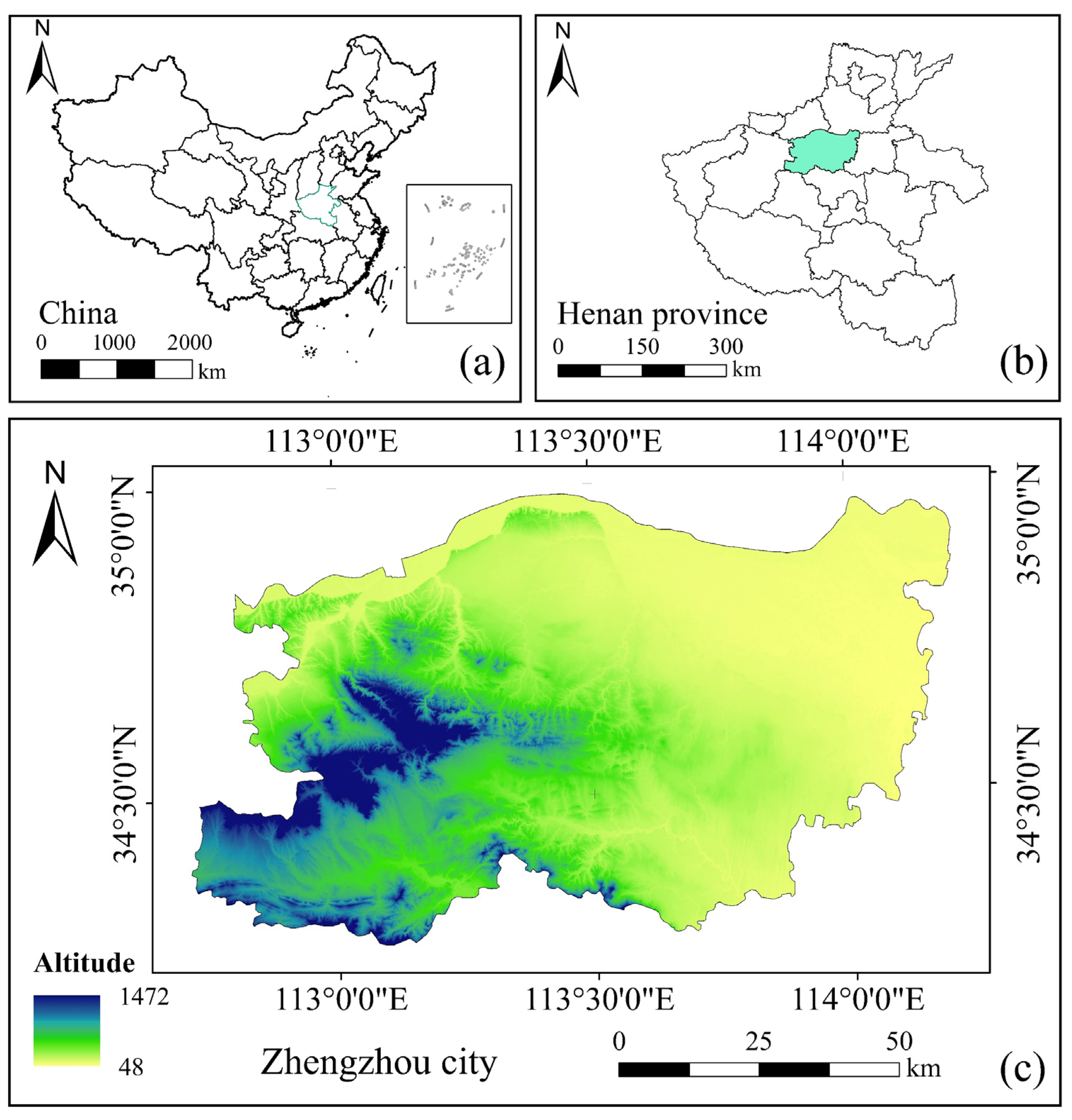
Zhengzhou (34°16′–34°58′ N, 112°42′–114°14′ E) is the capital city of Henan Province in central China with an area of 7567 km² (Figure 1). It is close to the Yellow River in the north, Song Mountain in the south, Kaifeng city in the east, and Luoyang city in the west. The terrain is high in the southwest and low in the northeast, descending in a ladder shape.

With the improvement in the comprehensive strength of Zhengzhou, its gross domestic product (GDP) has exceeded CNY 1.2 trillion in 2020, which leads to sustained population agglomeration and large consumption of land resources. According to the report of China’s seventh population census, as of 1 November 2020, the permanent resident population of Zhengzhou is approximately 12.6 million, and the urbanization rate is 78.4%. According to the notice on the scale of urban built-up areas in Zhengzhou in 2020 issued by Zhengzhou Municipal People’s Government, the central metropolitan area of Zhengzhou reached 709.69 km², and the urban built-up land reached 1284.89 km², an increase of 60.19% and 72.52%, respectively, compared with 2016. Therefore, Zhengzhou is a veritable, rapidly urbanizing metropolis.

Zhengzhou has a north temperate continental monsoon climate, with an annual mean temperature of 15.6 °C, a mean rainfall of 542.15 mm, and a frost-free period of 209 days. The main habitats of this metropolis are cultivated land, construction land, and forest land. Cultivated land accounts for the highest proportion of the total area and constitutes the leading matrix landscape of Zhengzhou, reflecting the critical position of agriculture in Zhengzhou. Built-up land is mainly distributed at the central core of the municipal jurisdiction, accounting for one-sixth of the total area. Forest land is mainly distributed in the western and southwestern mountains, including Mang Mountains, Song Mountains, and Fuxi Mountains, which constitute Zhengzhou’s main ecological barrier. These main types of habitats contain the resources and environments required for the survival and reproduction of organisms and ensure the food security and ecological security of the local residents.

With the continuous expansion of human economic activities, many farmlands and natural habitats in the suburbs of Zhengzhou have been gradually occupied, seriously damaging the stability of the urban ecosystem. Therefore, protecting urban habitats and promoting the social, economic, and ecological development of urban ecosystems have become the primary issues facing the government of this metropolis. Due to the variety of urban habitats and their hierarchical characteristics, it is complex and expensive to analyze all habitats at a comprehensive scale. In this case, the urban size, data availability, and planning operability are considered in our study. We finally chose the research scale range of 500 m to 2000 m to explore the key driving factors of urban habitat quality, which can also provide a foundation for further research in related fields of continuous subdivision of habitat scale and habitat planning.

3. Data Sources and Methods

3.1. Data Used

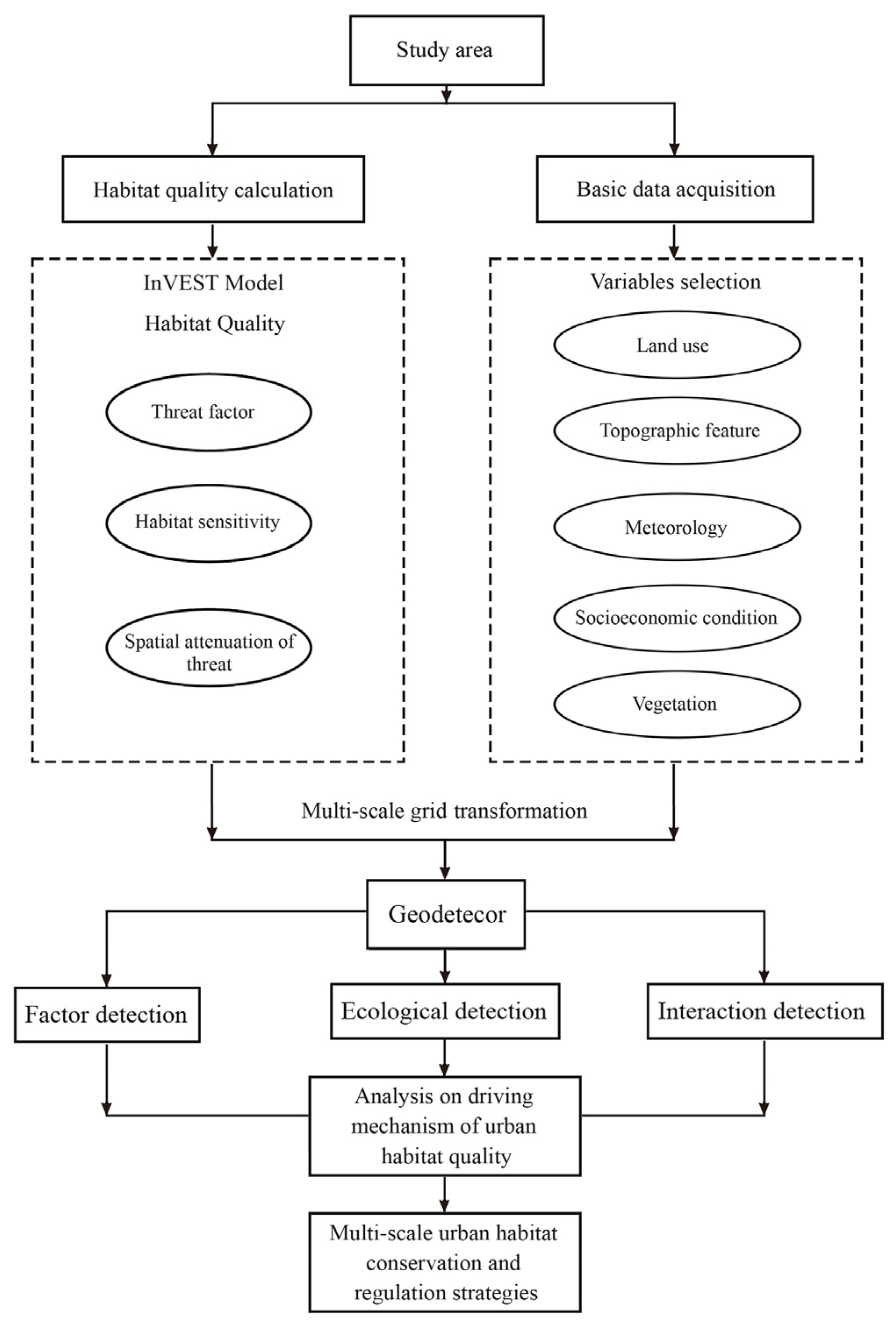
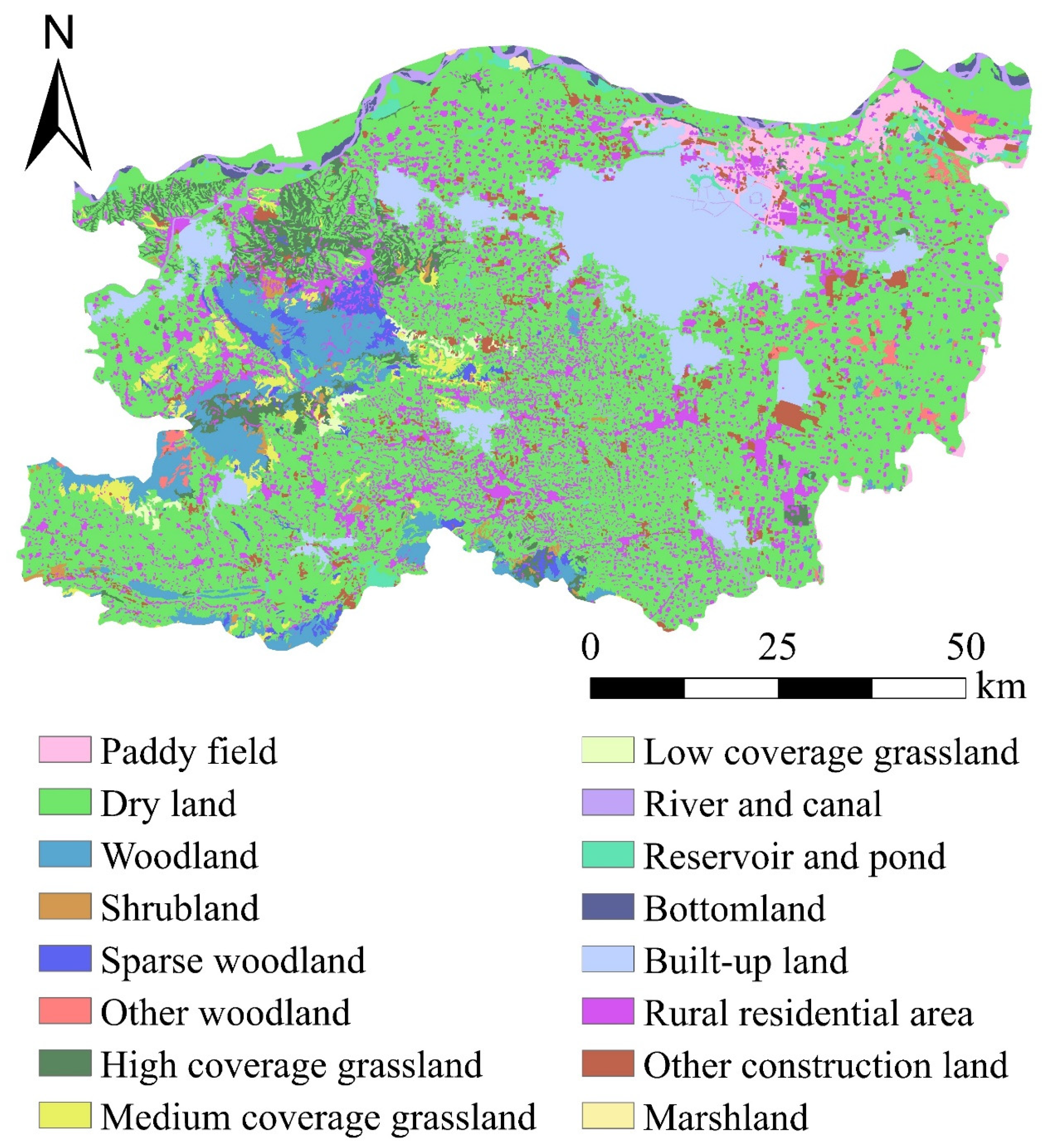
The workflow steps in our analysis are shown in Figure 2. The land use/cover change (LUCC) data needed to calculate the urban habitat quality are from Data Center for Resources and Environmental Sciences, Chinese Academy of Sciences (RESDC) [47]. We selected the LUCC data of Zhengzhou with a spatial resolution of 30 m in 2020 (Figure 3). It is worth noting that this data is based on the 2020 U.S. Landsat 8 remote sensing image data as the main information source and processed by human-computer interaction and visual interpretation technology. The interpretation process also involves the establishment of the LUCC classification system, the formulation of remote sensing interpretation marks and interpretation principles, and the quality inspection of interpretation results that can meet the requirements of scientific research.

The first classification is mainly divided into 6 categories of cultivated land, forest, grassland, water, construction land, and unused land according to the land resources and their utilization attributes; the second classification is mainly divided into 16 subcategories according to the natural attributes of land resources (

Table A1. Classification system of remote sensing monitoring data of LUCC in Zhengzhou.

Category	Subcategory	Meaning
Cultivated land	Paddy field	With water source guarantee and irrigation facilities for planting lotus roots and other aquatic crops
	Dry land	Cultivated land that mainly relies on natural precipitation to grow crops for vegetable cultivation
Forest	Woodland	Natural forests and plantations with a canopy closure > 30%; includes timber forests, economic forests, shelter forests, and other forest lands
	Shrubland	Low woodland and shrubland with canopy closure > 40% and height below 2 m
	Sparse woodland	Forest land with tree canopy closure of 10–30%
	Other woodland	Unformed forest afforestation land, nursery, and various garden plots, etc.
Grassland	High-coverage grassland	Natural and improved grasslands and mowing grass with a coverage > 50%; such grasslands generally have good water conditions, and the grass is grown densely
	Medium-coverage grassland	Natural and improved grasslands with a coverage of 20–50%; such grasslands generally lack water, and the grass cover is relatively sparse
	Low-coverage grassland	Natural grassland with a coverage of 5–20%; lacks water, is sparse, and animal husbandry utilization conditions are poor
Water	River and canal	Naturally formed or artificially excavated rivers and main trunk land below the water level throughout the year
	Reservoir and pond	Land below the perennial water level in the artificially constructed water storage area
	Bottomland	The land between the water level of rivers and lakes during the normal period and the water level of the flood period
Construction land	Built-up land	Built-up area mainly includes the central urban area and its direct jurisdictional cities and towns
	Rural residential area	Independent of rural settlements outside of cities and towns
	Other construction land	Mining, large industries, oil fields, salt works, quarries, traffic roads, airports, and other artificial lands
Unused land	Marshland	The terrain is flat and low-lying, with poor drainage, long-term humidity, seasonal ponding, or perennial ponding

). It should be added that the interpretation of results are multiple tests through random sampling of field survey points, random sampling of inspection lines and Kappa coefficient tests to ensure that the overall accuracy is not less than 90%, which has important practical significance in terms of applicability [48].

Before conducting studies on the driving mechanism of urban habitat quality, preliminary selection of suitable variables is necessary. It has been previously shown that land use, topographic feature, meteorology, socio-economic condition, and vegetation are widely considered to be five important aspects that affect ecological processes and patterns. Furthermore, according to the principles of availability and representativeness of ecological indicators, combined with the natural and socio-economic background of Zhengzhou, we selected 18 specific variables with independent ecological significance to analyze their impact mechanism on habitat quality at different spatial scales (

Table 1. List of variables selection.

Category	Variable	Data Acquisition Time
Land use	LUCC (X1)	2020
Topographic feature	Altitude (X2), slope (X3), aspect (X4), surface roughness (X5), and relief amplitude (X6)	2008
Meteorology	Daily mean temperature (X7), daily mean humidity (X8), daily mean wind speed (X9), daily mean wind direction (X10), and annual rainfall (X11)	2019
Socio-economic condition	Population (X12), GDP (X13), industrial output value (X14), agricultural output value (X15), and nighttime light (X16)	2019
Vegetation	NDVI (X17) and NPP (X18)	2019

). This process is in line with the exploratory and practical characteristics of scientific research.

Basic data of these variables in this study are derived from the following resources. We used the same LUCC data source mentioned earlier for calculating habitat quality. The topographic feature variable data were obtained by ArcGIS terrain analysis based on the digital elevation model (DEM) from the advanced land observing satellite project of the Japan Aerospace Research Institute with a spatial resolution of 12.5 m (http://www.jaxa.jp, accessed on 16 April 2021). The data of meteorology variables obtained by ArcGIS data conversion and ordinary Kriging interpolation are based on the hourly data of 7 national basic meteorological stations in Zhengzhou, which are from China National Meteorological Data Center. The population data are from world pop with a spatial resolution of 100 m (http://www.worldpop.org, accessed on 15 September 2020); GDP, industrial output values, and agricultural output values were retrieved from the statistical yearbook of Zhengzhou in 2020. The nighttime light data were from the Earth Observation Group’s annual VNL 2019 v.2 product, with a spatial resolution of 500 m (https://payneinstitute.mines.edu, accessed on 25 February 2021). The normalized difference vegetation index (NDVI) data was obtained through remote sensing image band operations from the Landsat-8 OLI/TIRS of the US Geological Survey with a spatial resolution of 30 m (https://earthexplorer.usgs.gov, accessed on 5 May 2021). The data of net primary productivity (NPP) were from the mod17a3 product of NASA EOS/MODIS with a spatial resolution of 500 m (https://e4ftl01.cr.usgs.gov, accessed on 24 April 2021).

It should be noted that due to different data acquisition methods and accessibility, meteorology and socio-economic condition data sources were annual data; the LUCC and vegetation data sources were obtained from the interpretation of remote sensing data in the near time; and the topographic feature data was regarded as unchanged in the short term. We default that they are in the same period and further focused our research on their impact on habitat quality on the different spatial scales.

3.2. Habitat Quality Calculation

InVEST is an ecosystem service assessment tool. Its habitat quality module is mainly based on LUCC data, stress factors, sensitivity to stress factors, and other parameters to assess habitat quality quantitatively (

Table A2. Habitat types and sensitivity of habitat types to each threat.

Habitat Type		Habitat Suitability	Threat Source
Main Category	Subcategory		Paddy Field	Dry Land	Urban Land	Rural Residential Land	Other Construction Land
Cultivated land	Paddy field	0.4	0	1	0.5	0.3	0.4
	Dry land	0.3	1	0	0.5	0.3	0.4
Forest	Woodland	1	0.8	0.9	0.9	0.8	0.8
	Shrubland	0.7	0.4	0.5	0.6	0.4	0.5
	Sparse woodland	0.6	0.8	0.9	0.5	0.7	0.8
	Other woodland	0.5	0.9	1	0.5	0.7	0.8
Grassland	High-coverage grassland	0.7	0.4	0.5	0.8	0.45	0.7
	Medium-coverage grassland	0.5	0.5	0.6	0.7	0.5	0.6
	Low-coverage grassland	0.3	0.7	0.9	0.6	0.55	0.5
Water	River and canal	1	0.7	0.5	0.7	0.6	0.6
	Reservoir and pond	0.8	0.8	0.4	0.8	0.7	0.7
	Bottomland	0.6	0	0	0.9	0.8	0.7
Construction land	Built-up land	0	0	0	0	0	0
	Rural residential land	0	0	0	0	0	0
	Other construction land	0	0	0	0	0	0
Unused land	Marshland	0.6	0.5	0.6	0.8	0.6	0.5

and

Table A3. Threats and their weight and the maximum distance of influence.

Threat Source	Relative Weight	Maximum Influence Distance (km)	Spatial Attenuation Function
Paddy field	0.4	4	Exponential
Dry land	0.3	4	Exponential
Built-up land	1	8	Exponential
Rural residential land	0.6	6	Exponential
Other construction land	0.8	5	Exponential

). The value range was 0–1, with values close to 1 meaning higher habitat quality, and those closer to 0, meaning lower habitat quality. We followed the recommended values in the InVEST model manual and relevant literature and set the model parameters in combination with the actual situation of the study area [11,49,50,51]. The main calculation formulas are as follows:

$$Q_{xj}=H_j\left[1-\left(\frac{D_{xj}^z}{D_{xj}^z+k^z}\right)\right]$$

(1)

where Q_xj is the habitat quality of the grid cell x in LUCC type j; k is the half-saturation constant; H_j is the habitat suitability of the land use type j; we hard code z = 2.5. The total threat level in grid cell x with LUCC type j is given by D_xj and it satisfies the following formula:

$$D_{xj}={\displaystyle {\sum }_{r=1}^R{\sum }_{y=1}^{Y_r}}\left(\frac{w_r}{{{\displaystyle \sum }}_{r=1}^R{w}_r}\right)r_y{i}_{rxy}{\beta }_x{S}_{jr}$$

(2)

where R represents the total threat sources (r = 1, 2, …, R); y indexes all grid cells on ’s raster map and Y_r indicates the set of grid cells on ’s raster map; a degradation source’s weight, w_r, indicates the relative destructiveness of a degradation source to all habitats; β_x represents the protection of society, law, etc., which is not taken into consideration in this study. The impact of threat r that originates in grid cell y, r_y, on habitat in grid cell x is given by i_rxy. Generally, we assume that the spatial attenuation of the impact of threat sources on the habitat quality is exponential and its variation with distance satisfies the following formula:

$$i_{rxy}=exp\left[-\left(\frac{2.99}{d_{r max}}\right)d_{xy}\right]$$

(3)

where d_xy is the linear distance between grid cell x and grid cell y, and d_{r max} is the maximum impact distance of threat source r.

3.3. Geodetector

Geodetector is used to measure the spatial differentiation of a certain attribute and explore its driving mechanism. Compared with traditional models, we can use it to analyze the relationship between variables without the assumption of linearity or the collinearity of variables, including four components: factor detection, interactive detection, ecological detection, and risk area detection; the first three are mainly used in our study (http://www.geodetector.cn, accessed on 27 May 2021).

Factor detection can measure the determinant power of an explanatory variable X of dependent variable Y which is used to compute the contribution of driving factor to the spatial differentiation of urban habitat quality by q statistic. The formula is as follows:

$$q=1-\frac{{{\displaystyle \sum }}_{h=1}^L{N}_h^{ }{\sigma }_h^2}{N{\sigma }^2}$$

(4)

where L is the strata number of X or Y (h = 1, 2, …, L). N_h and N are the unit number of stratum h and the whole region, respectively; ${\sigma }_h^2$ and ${\sigma }^2$ are the variances of the Y values of stratum h and the whole region, respectively; the range of q-value is (0, 1). The larger the q-value, the more obvious the spatial differentiation of Y; If the stratification is generated by X, the larger the q-value, the stronger the explanatory power of X to Y.

Ecological detection is used to compare whether there is a significant difference between X_a and X_b on the spatial distribution of Y by F statistics. The formula is as follows:

$$F=\frac{N_a\left(N_b-1\right)SS{W}_a}{N_b\left(N_a-1\right)SS{W}_b}$$

(5)

$$SS{W}_a={\displaystyle \sum }_{h=1}^{L_a}{N}_h^{ }{\sigma }_h^2$$

(6)

$$SS{W}_b={\displaystyle \sum }_{h=1}^{L_b}{N}_h^{ }{\sigma }_h^2$$

(7)

where N_a and N_b represent the sample size of factor X_a and factor X_b, respectively; SSW_a and SSW_b represent sum of variances for each stratum of X_a and X_b, respectively; and L_a and L_b represent the strata number of X_a and X_b, respectively. The null hypothesis is H₀: SSW_a = SSW_b. If the H₀ is rejected to a significant level, it indicates that there are significant differences in the impact of X_a and X_b on the spatial distribution of Y.

Interaction detection is used to judge whether the combination of factors X_a and X_b increase or decrease the explanatory power of the dependent variable Y or whether the impacts of these two factors on Y are independent. The assessment method is to first calculate the q-values of Y for two factors, X_a and X_b, respectively: q(X_a) and q(X_b), and to calculate the q-values when they interact: q(X_a ∩ X_b). Further compare q(X_a), q(X_b) and q(X_a ∩ X_b) to conclude whether there is an interaction between these two factors, the strength of their interaction, positive or negative effect, linearity or nonlinearity, etc. The corresponding interaction relationship and judgment basis are shown in

Table 2. Judgment basis of interaction type.

Interaction	Judgment Basis
Nonlinear weakening	q(Xa ∩ Xb) < Min[q(Xa), q(Xb)]
Single-factor nonlinear weakening	Min[q(Xa), q(Xb)] < q(Xa ∩ Xb) < Max[q(Xa), q(Xb)]
Double-factor enhanced	q(Xa ∩ Xb) > Max[q(Xa), q(Xb)]
Independence	q(Xa ∩ Xb) = q(Xa) + q(Xb)
Nonlinear enhanced	q(Xa ∩ Xb) > q(Xa) + q(Xb)

below.

It should be noted that type variables are better than continuous variables in the Geodetector software settings. Therefore, the impact factor index we selected is divided into ten levels using the geometric interval method to divide the continuous index data at different grid-scales.

4. Results

4.1. Distribution Characteristics of Habitat Quality at Different Grid-Scales

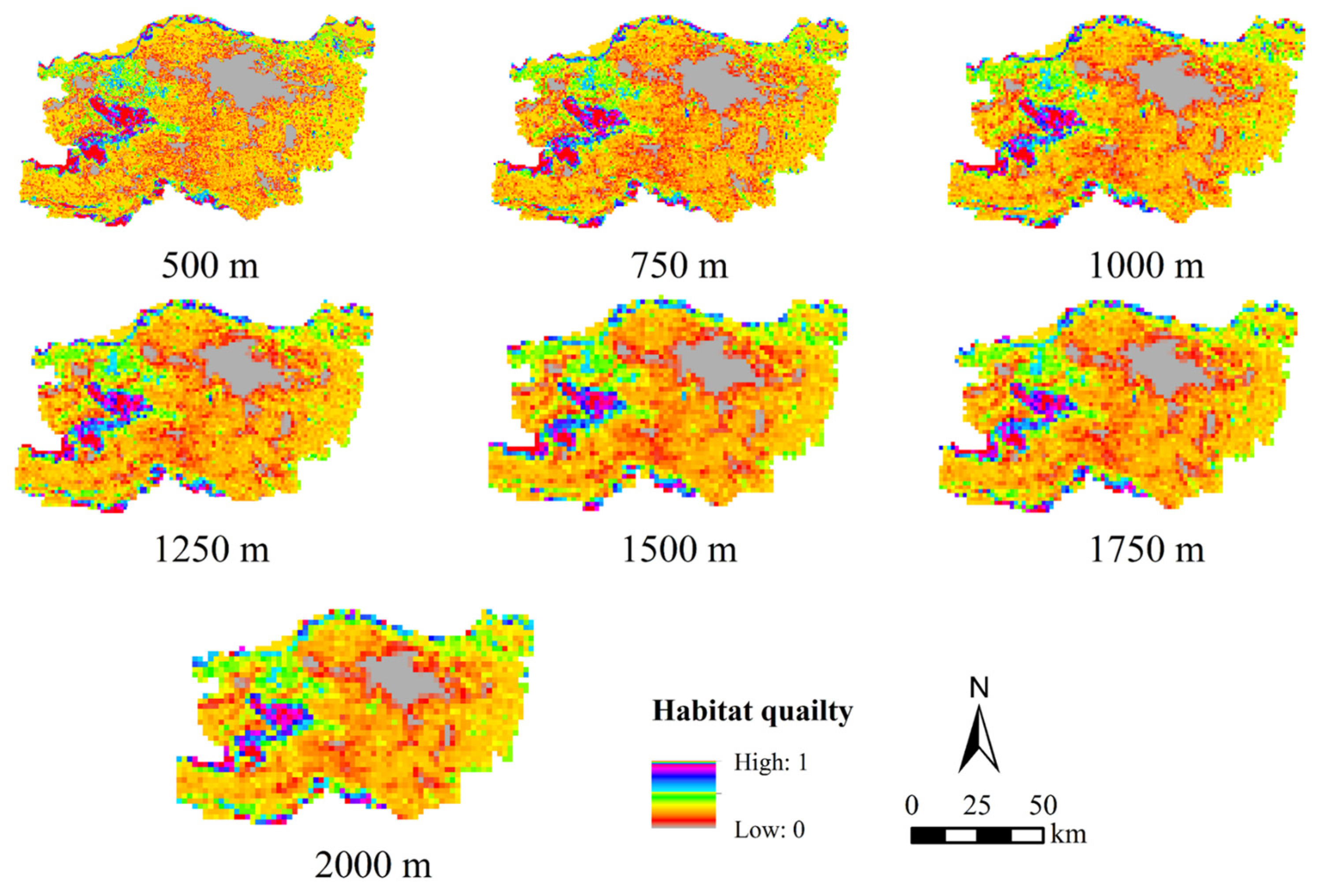
With the increase of grid-scales, the mean habitat quality of Zhengzhou fluctuated between 0.293 and 0.295; the habitat quality of the urban–rural transition zone close to the central urban area decreased significantly, while the habitat quality of vast wilderness far away from the central urban area continued to rise (Figure 4). Notably, grid-scale had little impact on the overall value of habitat quality but had a greater impact on the spatial attributes of habitat quality. That is, the distribution of urban habitat quality showed obvious spatial heterogeneity at different grid-scales.

4.2. Analysis of the Impact Intensity of Factors

Factor detection is used to reveal the impact intensity of each factor on habitat quality (

Table 3. q-value of factors at different grid-scales.

Factor	Grid-Scale							Mean q-Value	Standard Deviation
	500 m	750 m	1000 m	1250 m	1500 m	1750 m	2000 m
X1	0.877	0.851	0.839	0.832	0.823	0.808	0.795	0.832	0.027
X2	0.312	0.333	0.352	0.367	0.380	0.379	0.401	0.361	0.030
X3	0.423	0.457	0.495	0.515	0.521	0.528	0.516	0.494	0.039
X4	0.082	0.097	0.108	0.119	0.134	0.149	0.153	0.120	0.027
X5	0.414	0.445	0.478	0.497	0.501	0.525	0.522	0.483	0.041
X6	0.415	0.446	0.470	0.489	0.495	0.502	0.513	0.476	0.035
X7	0.084	0.092	0.099	0.101	0.107	0.104	0.118	0.101	0.011
X8	0.056	0.061	0.067	0.068	0.068	0.074	0.079	0.067	0.008
X9	0.085	0.093	0.098	0.104	0.106	0.113	0.115	0.102	0.011
X10	0.077	0.084	0.089	0.095	0.097	0.099	0.104	0.092	0.009
X11	0.039	0.043	0.044	0.046	0.049	0.053	0.055	0.047	0.006
X12	0.317	0.358	0.381	0.405	0.428	0.444	0.460	0.399	0.051
X13	0.122	0.122	0.122	0.127	0.129	0.133	0.127	0.126	0.004
X14	0.079	0.084	0.082	0.088	0.099	0.099	0.111	0.092	0.011
X15	0.128	0.138	0.144	0.152	0.161	0.170	0.171	0.152	0.016
X16	0.403	0.428	0.452	0.476	0.487	0.507	0.522	0.468	0.043
X17	0.481	0.522	0.548	0.536	0.561	0.569	0.592	0.544	0.036
X18	0.080	0.080	0.084	0.085	0.098	0.088	0.100	0.088	0.008

). The mean q-value ranking of 18 factors on habitat quality at 7 grid-scales from 500 m to 2000 m: X₁ (0.832) > X₁₇ (0.544) > X₃ (0.494) > X₅ (0.483) > X₆ (0.476) > X₁₆ (0.468) > X₁₂ (0.399) > X₂ (0.361) > X₁₅ (0.152) > X₁₃ (0.126) > X₄ (0.120) > X₉ (0.102) > X₇ (0.101) > X₁₀ (0.0921) > X₁₄ (0.0917) > X₁₈ (0.088) > X₈ (0.067) > X₁₁ (0.047). LUCC and NDVI were the dominant factors affecting habitat quality; their q-values were 0.832 and 0.544, respectively. Altitude, slope, aspect, relief amplitude, population, and nighttime light were the secondary factors affecting habitat quality, and their q-values all exceeded 0.3. With the increase of grid-scale, the impact of LUCC on the habitat quality decreased, while the other factors increased.

The impact intensity of factors on habitat quality at different grid-scales shows significant differences. Slope, surface roughness, population, nighttime light, and NDVI had higher mean q-values, while they were more sensitive to scale variations, and the q-value change interval was greater than 0.1. When the grid-scale was 1000 m, the q-values of the slope, surface roughness, and NDVI were closer to their mean q-value, respectively; when the grid-scale was 1250 m, the q-values of population and nighttime light were closer to their mean q-value, respectively. Therefore, at the grid-scale of 1000 to 1250 m, the impacts of the dominant factors on habitat quality were closer to their mean level of multiple scales. We further speculate that this scale range should be used to efficiently carry out follow-up research on the driving mechanism of habitat quality in Zhengzhou which can fully consider the scale effect of spatial error.

4.3. Analysis on the Difference in the Impact of Factors

Ecological detection is used to explore whether there is a significant difference between the respective impact of two factors on habitat quality at different grid-scales (p < 0.05). We define the following three types of representations: with the variation of grid-scales, the respective impact of two factors varies between significant difference and no significant difference, represented by Z; there has always been no significant difference between the respective impact of the two factors, represented by N; There has always been a significant difference between the respective impact of two factors, represented by Y.

Eighteen factors constitute a total of 153 comparison pairs (

Table 4. Significance test of the impact on habitat quality of factors.

	X1	X2	X3	X4	X5	X6	X7	X8	X9	X10	X11	X12	X13	X14	X15	X16	X17
X2	Y
X3	Y	Y
X4	Y	Y	Y
X5	Y	Y	Z	Y
X6	Y	Y	Z	Y	N
X7	Y	Y	Y	N	Y	Y
X8	Y	Y	Y	Y	Y	Y	Z
X9	Y	Y	Y	N	Y	Y	N	Z
X10	Y	Y	Y	N	Y	Y	N	Z	N
X11	Y	Y	Y	Y	Y	Y	Y	Z	Y	Z
X12	Y	Z	Y	Y	Y	Y	Y	Y	Y	Y	Y
X13	Y	Y	Y	Z	Y	Y	Z	Z	Z	Y	Y	Y
X14	Y	Y	Y	N	Y	Y	N	Z	N	N	Z	Y	Z
X15	Y	Y	Y	Y	Y	Y	Y	Y	Y	Y	Y	Y	N	Y
X16	Y	Y	Z	Y	Z	Z	Y	Y	Y	Y	Y	Y	Y	Y	Y
X17	Y	Y	Y	Y	Y	Y	Y	Y	Y	Y	Y	Y	Y	Y	Y	Y
X18	Y	Y	Y	Z	Y	Y	N	Z	N	N	Z	Y	Z	N	Y	Y	Y

). With the variation of grid-scales, there were a total of 22 Z-type, of which the comparison pairs involved by daily mean humidity, annual rainfall, or GDP account for 68.2%; there were a total of 16 N-type, of which the comparison pairs involved by daily mean temperature, daily mean wind speed, or daily mean wind direction account for 75%; there were a total of 115 Y-type, of which the comparison pairs involved by LUCC or NDVI all belong to this type. This result indicated that there has always been a significant difference between the respective impact of two factors. In summary, the impact of each factor on the spatial distribution of habitat quality was different, and the difference between most factors was always significant regardless of the variation of grid-scales.

4.4. Analysis of the Interaction of Factors

Interaction detection was used to calculate superimposed q-values of 153 interaction pairs composed of 18 factors on the habitat quality. Coefficient of variation (CV) was used to quantitatively analyze whether there was a significant difference in the superimposed q-value at different grid-scales. Generally, a CV ≤ 0.1 indicates that the superimposed q-value has weak variation; 0.1 < CV < 1 has a moderate variation; and CV ≥ 1 has a strong variation. The results are shown in

Table 5. Mean superimposed q-value and interaction type between 18 factors at 7 grid-scales from 500 m to 2000 m. * indicates 0.1 < CV < 1, and no * indicates CV < 0.1; Δ: double-factor enhanced; □: nonlinear enhanced; ●: double-factor enhanced or nonlinear enhanced.

	X1	X2	X3	X4	X5	X6	X7	X8	X9	X10	X11	X12	X13	X14	X15	X16	X17	X18
X1	-	Δ	Δ	Δ	Δ	Δ	Δ	Δ	Δ	Δ	Δ	Δ	Δ	Δ	Δ	Δ	Δ	Δ
X2	0.855	-	Δ	Δ	Δ	Δ	□	□	Δ	□		Δ	●	□	●	Δ	Δ	Δ
X3	0.861	0.555	-	Δ	Δ	Δ	Δ	●	Δ	Δ	□	Δ	Δ	●	Δ	Δ	Δ	●
X4	0.844	0.434 *	0.519	-	Δ	Δ	Δ	□	Δ	Δ	□	Δ	Δ	●	Δ	Δ	Δ	□
X5	0.864	0.547	0.551	0.527	-	Δ	Δ	□	Δ	Δ	□	Δ	Δ	Δ	Δ	Δ	Δ	●
X6	0.862	0.527	0.538	0.517	0.521	-	Δ	□	Δ	Δ	●	Δ	Δ	Δ	Δ	Δ	Δ	●
X7	0.850	0.494	0.558	0.197 *	0.552	0.540	-	□	□	□	□	Δ	□	□	●	Δ	□	●
X8	0.853	0.479	0.564	0.203 *	0.562	0.554	0.318 *	-	□	□	□	□	□	□	●	□	□	□
X9	0.847	0.449	0.573	0.211 *	0.563 *	0.548	0.224 *	0.335 *	-	□	□	Δ	□	□	●	●	Δ	□
X10	0.850	0.530	0.564	0.204 *	0.556	0.551	0.249 *	0.294 *	0.327 *	-	□	Δ	□	□	□	□	●	□
X11	0.850	0.514	0.570	0.181 *	0.563	0.550	0.257 *	0.266 *	0.343	0.313 *	-	□	□	□	□	Δ	□	□
X12	0.863	0.561 *	0.628	0.470 *	0.621	0.612	0.483 *	0.477 *	0.464 *	0.471 *	0.468 *	-	Δ	Δ	Δ	Δ	Δ	Δ
X13	0.847	0.495	0.585	0.237 *	0.576	0.556	0.268 *	0.308	0.300	0.276	0.252	0.482	-	Δ	Δ	Δ	●	□
X14	0.846	0.463	0.573	0.217 *	0.558	0.541	0.261 *	0.263 *	0.263 *	0.260 *	0.254 *	0.479 *	0.188 *	-	Δ	Δ	●	□
X15	0.847	0.506 *	0.589	0.261 *	0.585	0.566	0.269 *	0.312 *	0.251 *	0.272 *	0.308 *	0.443 *	0.228 *	0.227 *	-	Δ	Δ	□
X16	0.868	0.589	0.665	0.506 *	0.663	0.654	0.555	0.540	0.564	0.575	0.499	0.563	0.524	0.525	0.519	-	Δ	□
X17	0.875	0.607	0.660	0.613	0.652	0.645	0.642	0.654	0.583	0.639	0.667	0.671	0.657	0.635	0.635	0.700	-	Δ
X18	0.848	0.470 *	0.585	0.291	0.565	0.556 *	0.333 *	0.242 *	0.304 *	0.290 *	0.270 *	0.476 *	0.313 *	0.251	0.276	0.585	0.605	-

. All interaction pairs are characterized as double-factor enhanced type or nonlinear enhanced type at seven grid-scales from 500 m to 2000 m, indicating that the interaction effect of two factors was greater than the independent effects of either one on habitat quality. The mean q-values of the 17 interaction pairs involving LUCC were greater than 0.8. The mean q-values of the 91 interaction pairs involving altitude, slope, surface roughness, relief amplitude, population, nighttime light, and NDVI were greater than 0.4.

According to the CV results, the superimposed q-values of the interaction pairs composed of LUCC, slope, relief amplitude, and NDVI showed weak variation at seven grid-scales. The superimposed q-values of more than a third of the interaction pairs showed moderate variation at seven grid-scales, and these interaction pairs were mainly involved with daily mean temperature, daily mean humidity, daily mean wind speed, daily mean wind direction, population, industrial output value, and agricultural output value involved. Additionally, at different grid-scales, the types of most of the interaction pairs remain the same, that is, either double-factor enhanced type or nonlinear enhanced type, which accounted for 56.9% and 32.0% of the total. There were also a few interaction pairs that varied between double-factor enhanced type and nonlinear enhanced type with the variation of grid-scales, accounting for 11.1%. Taken overall, the superimposed impact of two factors on the spatial distribution of habitat quality was greater than the impact of the single factor.

5. Discussion

Urban habitat quality and its driving mechanisms are characterized by spatial nonstationarity, spatial heterogeneity, and spatial dependence. In this study, the impact of LUCC on habitat quality in Zhengzhou was the most prominent at different grid-scales, indicating that human activities are increasingly interfering with urban habitat. Some studies have shown that urban land spatial layout had a great impact on the quality of the ecological environment, which is consistent with our results [52,53,54]. This study shows that cultivated land and woodland in the periphery of Zhengzhou’s central urban area are occupied by construction land to varying degrees; the large-scale loss and fragmentation of the original habitat have significantly reduced the quality of the habitat. Meanwhile, in order to deal with these problems, the government continued to advance the adjustment of the industrial and energy structures, accelerate the construction of a natural reserve system with national parks as the main body, and expand the area of the natural reserve. Hence, the habitat quality of woodland in western Zhengzhou, including the Dengfeng district, Xinmi district, and Gongyi district, were improved to some extent. Briefly, urban habitat quality is closely related to urban land utilization layout. Urban land utilization layout can directly change the structure, composition, and function of urban habitats [55,56].

Topographic features are the second most prominent driving factor leading to the spatial differentiation of habitat quality in Zhengzhou. This specifically includes the ecological factors of altitude, slope, aspect, relief, and amplitude. Habitats with complex topographic features, such as forests, rivers, etc., can provide favorable space for animals and plants rather than humans. Usually, these habitats are less disturbed by humans and have higher habitat quality [57]. In contrast, habitats with gentle topographic features, such as cultivated and construction land, are greatly disturbed by human activities and have lower habitat quality. This is the result of only considering the construction cost in the process of urban expansion. If no further control measures are taken, it will inevitably lead to the continuous occupation of farmland, grassland, woodland, and other habitats on the eastern plain areas, which will pose a great threat to the ecological security of Zhengzhou.

Next to land use and topographic features, nighttime light and NDVI are also driving factors of urban habitat quality that cannot be ignored. Nighttime light can intuitively reflect the intensity of human interference with nature. Excessive nighttime light will inevitably disrupt the circadian rhythm of urban plants and the rules of animal foraging and hiding. Therefore, we must pay attention to the habitat degradation and habitat quality degradation caused by nighttime light pollution and carry out follow-up quantitative research. NDVI is an important indicator to measure the quality of urban vegetation. Moreover, urban vegetation directly participates in the material cycle and energy flow of the ecosystem. Protecting and restoring urban vegetation is of great significance for improving habitat quality. Based on the results of these prominent ecological factors affecting urban habitat quality and some laws among them, we put forward the key research directions of Zhengzhou habitat protection according to the following local conditions.

(1) Adjusting urban land use structure based on the functional orientation and ecological carrying capacity of Zhengzhou. We should strictly adhere to the delineated red line of ecological protection, make rational spatial layouts based on this premise, and divide Zhengzhou’s ecological space, production space, and living space. According to areas with low habitat quality, we should strictly control the scale of new construction land, the amount of cultivated land, and the scope of the prohibition of reclamation, and strive to improve the level of economic and intensive utilization of construction land to ensure the sustainable development of urban habitat. For example, from the perspective of efficient utilization and ecological control of land use, Zhengzhou is divided into six ecological function zones: the central urban construction area, the northern soil and water conservation area, the western mountain ecological protection area, the southwestern natural reserve area, the southern farmland protection area, and the eastern new urban area.

(2) Applying nature-based solutions to restore native biodiversity and damaged natural habitats in Zhengzhou. We can explore the optimal grid of the urban habitat network and its quantitative graded management theory to promote the construction of near-natural urban habitats. In addition, it is necessary to strengthen the rejuvenation and reintroduction of local biological populations, control the invasion of alien species, and guide the behavior of residents in multiple ways to reduce the impact of human activities on urban biodiversity. For example, native botanical gardens should be planned around the countryside, bird sanctuaries should be established along the Yellow River wetland, targeted sanctuaries should be established for local unique or national protected plants and animals that are concentrated in Song Mountains and Mang Mountains.

(3) Establish a systematic thinking model for multi-level urban habitat sustainability. We should integrate multi-scale urban habitat mapping and assessment into the whole process of urban planning and design to balance the needs of human society development and nature protection at different spatial scales. For example, at the block scale, we should strengthen the three-dimensional greening of hard facilities such as overpasses, viaducts, and retaining walls, and make full use of the potential valuable habitats around the structures; at the metropolitan scale, we should protect important habitat patches and ecological corridors, such as western Song Mountains, northern Yellow River wetland, southwestern Baisha reservoir and eastern Yanming Lake wetland, etc.

Notably, we found some dominant factors affecting the quality of urban habitat and some of their interrelationship characteristics, which can only use as a reference for the planning of Zhengzhou City in this specific period. The quantitative research on the driving mechanism of urban habitat quality at different spatial scales is a very complex task, which requires longer-term exploration and accumulation of rich data for verification. Some imperfections in this experiment are worth mentioning. For example, urban habitat quality may be affected by social policies, physical and chemical properties of soil, microorganisms, air quality, etc., which were not considered due to the limitations of data acquisition in this study [58,59]. Additionally, we only selected the grid-scales from 500 m to 2000 m to analyze the driving factors of habitat quality because the accuracy of vector data will decrease with wider grid-scales.

A follow-up study should focus on how to consider more potential driving factors and techniques for reducing the accuracy loss of vector data in the process of wider grid-scale transformations to provide support for the multi-scale regulation of urban habitat and biodiversity. With regards to this, the construction of more fixed sample plots to monitor various factors will provide the basic feasibility for establishing a conversion model between remote sensing data and field survey data [60]. Furthermore, using indicator species and some environmental characteristic variables (species diversity, niche, etc.) to measure habitat quality, which will make the experimental results more visible and convincing.

6. Conclusions

In this paper, the driving mechanism of spatial differentiation of habitat quality in Zhengzhou is explored by InVEST model and Geodetector software. Further, the impact differences and interactions of various factors on urban habitat quality at different grid-scales were analyzed. Our conclusions are as follows:

(1) The overall habitat quality in the study area fluctuated slightly between 0.293 and 0.295 with the variation of grid-scales. LUCC, altitude, slope, surface roughness, relief amplitude, population, nighttime light, and NDVI were the dominant factors affecting the spatial differentiation of habitat quality. With the variation of grid-scales, these mean q statistics were more than 0.3.

(2) The impacts of slope, surface roughness, population, nighttime light, and NDVI on habitat quality are highly sensitive to grid-scale variations. Fully considering the errors caused by the spatial data of these factors, it is a suitable choice to efficiently analyze the impacts of the dominant ecological factors on urban habitat quality at the spatial scale of 1000 to 1250 m, and the results are closest to the mean level of multiple spatial scales.

(3) The impact of each factor on the spatial distribution of habitat quality is different, and the difference between most factors has always been significant regardless of the variation of grid-scales. The superimposed impact of two factors on the spatial distribution of habitat quality is greater than the impact of the single factor.

(4) Our study innovatively explored the spatial differentiation characteristics of urban habitat quality and the driving characteristics of 18 ecological factors on habitat quality at different spatial scales, which will be an effective and repeatable analytical idea for planning industry workers. In the future, more factors and a wider range of grid-scales will be considered to quantitatively analyze the internal mechanism of habitat quality differentiation in Zhengzhou to provide data support for multi-scale urban habitats ecological protection and restoration in similar cities.

References

- Long, H.; Liu, Y.; Hou, X.; Li, T.; Li, Y. Effects of Land Use Transitions Due to Rapid Urbanization on Ecosystem Services: Implications for Urban Planning in the New Developing Area of China. Habitat Int. 2014, 44, 536–544. [Google Scholar] [CrossRef]
- Pickett, S.T.A.; Cadenasso, M.L.; Childers, D.L.; Mcdonnell, M.J.; Zhou, W. Evolution and Future of Urban Ecological Science: Ecology in, of, and for the City. Ecosyst. Health Sustain. 2016, 2, e01229. [Google Scholar] [CrossRef]
- Barreteau, O.; Giband, D.; Schoon, M.; Cerceau, J.; DeClerck, F.; Ghiotti, S.; James, T.; Masterson, V.A.; Mathevet, R.; Rode, S.; et al. Bringing Together Social-Ecological System and Territoire Concepts to Explore Nature-Society Dynamics. Ecol. Soc. 2016, 21, art42. [Google Scholar] [CrossRef] [Green Version]
- Pickett, S.T.A.; Cadenasso, M.L.; Grove, J.M.; Boone, C.G.; Groffman, P.M.; Irwin, E.; Kaushal, S.S.; Marshall, V.; McGrath, B.P.; Nilon, C.H.; et al. Urban Ecological Systems: Scientific Foundations and a Decade of Progress. J. Environ. Manag. 2011, 92, 331–362. [Google Scholar] [CrossRef] [PubMed]
- Wang, Z.; Deng, X.; Wong, C.; Li, Z.; Chen, J. Learning Urban Resilience from a Social-Economic-Ecological System Perspective: A Case Study of Beijing from 1978 to 2015. J. Clean. Prod. 2018, 183, 343–357. [Google Scholar] [CrossRef]
- Tripp, E.A.; Lendemer, J.C.; McCain, C.M. Habitat Quality and Disturbance Drive Lichen Species Richness in a Temperate Biodiversity Hotspot. Oecologia 2019, 190, 445–457. [Google Scholar] [CrossRef]
- Vaz, A.S.; Marcos, B.; Gonçalves, J.; Monteiro, A.; Alves, P.; Civantos, E.; Lucas, R.; Mairota, P.; Garcia-Robles, J.; Alonso, J.; et al. Can We Predict Habitat Quality from Space? A Multi-Indicator Assessment Based on an Automated Knowledge-Driven System. Int. J. Appl. Earth Obs. Geoinf. 2015, 37, 106–113. [Google Scholar] [CrossRef]
- Gao, Y.; Ma, L.; Liu, J.; Zhuang, Z.; Huang, Q.; Li, M. Constructing Ecological Networks Based on Habitat Quality Assessment: A Case Study of Changzhou, China. Sci. Rep. 2017, 7, 46073. [Google Scholar] [CrossRef]
- Štefunková, Z.; Macura, V.; Škrinár, A.; Majorošová, M.; Doláková, G.; Halaj, P.; Petrová, T. Evaluation of the Methodology to Assess the Influence of Hydraulic Characteristics on Habitat Quality. Water 2020, 12, 1131. [Google Scholar] [CrossRef] [Green Version]
- Neumann, C.; Weiss, G.; Schmidtlein, S.; Itzerott, S.; Lausch, A.; Doktor, D.; Brell, M. Gradient-Based Assessment of Habitat Quality for Spectral Ecosystem Monitoring. Remote Sens. 2015, 7, 2871–2898. [Google Scholar] [CrossRef] [Green Version]
- Wang, H.; Tang, L.; Qiu, Q.; Chen, H. Assessing the Impacts of Urban Expansion on Habitat Quality by Combining the Concepts of Land Use, Landscape, and Habitat in Two Urban Agglomerations in China. Sustainability 2020, 12, 4346. [Google Scholar] [CrossRef]
- Wang, L.; Yu, D.; Liu, Z.; Yang, Y.; Zhang, J.; Han, J.; Mao, Z. Study on NDVI Changes in Weihe Watershed Based on CA-Markov Model. Geol. J. 2018, 53, 435–441. [Google Scholar] [CrossRef]
- Moreno, R.; Zamora, R.; Molina, J.R.; Vasquez, A.; Herrera, M.Á. Predictive Modeling of Microhabitats for Endemic Birds in South Chilean Temperate Forests Using Maximum Entropy (Maxent). Ecol. Inform. 2011, 6, 364–370. [Google Scholar] [CrossRef]
- Brown, G.; Brabyn, L. The Extrapolation of Social Landscape Values to a National Level in New Zealand Using Landscape Character Classification. Appl. Geogr. 2012, 35, 84–94. [Google Scholar] [CrossRef]
- Berta Aneseyee, A.; Noszczyk, T.; Soromessa, T.; Elias, E. The InVEST Habitat Quality Model Associated with Land Use/Cover Changes: A Qualitative Case Study of the Winike Watershed in the Omo-Gibe Basin, Southwest Ethiopia. Remote Sens. 2020, 12, 1103. [Google Scholar] [CrossRef] [Green Version]
- Nematollahi, S.; Fakheran, S.; Kienast, F.; Jafari, A. Application of InVEST Habitat Quality Module in Spatially Vulnerability Assessment of Natural Habitats (Case Study: Chaharmahal and Bakhtiari Province, Iran). Environ. Monit. Assess. 2020, 192, 487. [Google Scholar] [CrossRef]
- Zhang, H.; Zhang, C.; Hu, T.; Zhang, M.; Ren, X.; Hou, L. Exploration of Roadway Factors and Habitat Quality Using InVEST. Transp. Res. Part D Transp. Environ. 2020, 87, 102551. [Google Scholar] [CrossRef]
- Zhou, X.; Xiao, L.; Lu, X.; Sun, D. Impact of Road Transportation Development on Habitat Quality in Economically Developed Areas: A Case Study of Jiangsu Province, China. Growth Change 2020, 51, 852–871. [Google Scholar] [CrossRef]
- He, J.; Huang, J.; Li, C. The Evaluation for the Impact of Land Use Change on Habitat Quality: A Joint Contribution of Cellular Automata Scenario Simulation and Habitat Quality Assessment Model. Ecol. Model. 2017, 366, 58–67. [Google Scholar] [CrossRef]
- Wang, X.; Sun, Y.; Zhang, L.; Mei, Y. Spatial Variation and Influence Factor Analysis of Soil Heavy Metal As Based on GeoDetector. Stoch. Environ. Res. Risk Assess. 2021, 35, 2021–2030. [Google Scholar] [CrossRef]
- Liu, Y.; Cao, X.; Li, T. Influence of Accessibility on Land Use and Landscape Pattern Based on Mapping Knowledge Domains: Review and Implications. J. Adv. Transp. 2020, 2020, 7985719. [Google Scholar] [CrossRef]
- Sila-Nowicka, K.; Thakuriah, P. Multi-Sensor Movement Analysis for Transport Safety and Health Applications. PLoS ONE 2019, 14, e0210090. [Google Scholar] [CrossRef]
- Chen, L.; Shen, W. Spatiotemporal Differentiation of Urban-Rural Income Disparity and Its Driving Force in the Yangtze River Economic Belt during 2000–2017. PLoS ONE 2021, 16, e0245961. [Google Scholar] [CrossRef] [PubMed]
- Wang, H.; Qin, F.; Xu, C.; Li, B.; Guo, L.; Wang, Z. Evaluating the Suitability of Urban Development Land with a Geodetector. Ecol. Indic. 2021, 123, 107339. [Google Scholar] [CrossRef]
- Wang, R.; Xia, B.; Dong, S.; Li, Y.; Li, Z.; Ba, D.; Zhang, W. Research on the Spatial Differentiation and Driving Forces of Eco-Efficiency of Regional Tourism in China. Sustainability 2021, 13, 280. [Google Scholar] [CrossRef]
- Xia, B.; Dong, S.; Ba, D.; Li, Y.; Li, F.; Liu, H.; Li, Z.; Zhao, M. Research on the Spatial Differentiation and Driving Factors of Tourism Enterprises’ Efficiency: Chinese Scenic Spots, Travel Agencies, and Hotels. Sustainability 2018, 10, 901. [Google Scholar] [CrossRef] [Green Version]
- Alamdar, F.; Kalantari, M.; Rajabifard, A. An Evaluation of Integrating Multisourced Sensors for Disaster Management. Int. J. Digit. Earth 2015, 8, 727–749. [Google Scholar] [CrossRef]
- Breunig, M.; Bradley, P.E.; Jahn, M.; Kuper, P.; Mazroob, N.; Rösch, N.; Al-Doori, M.; Stefanakis, E.; Jadidi, M. Geospatial Data Management Research: Progress and Future Directions. ISPRS Int. J. Geo-Inf. 2020, 9, 95. [Google Scholar] [CrossRef] [Green Version]
- Gu, J.; Liang, L.; Song, H.; Kong, Y.; Ma, R.; Hou, Y.; Zhao, J.; Liu, J.; He, N.; Zhang, Y. A Method for Hand-Foot-Mouth Disease Prediction Using GeoDetector and LSTM Model in Guangxi, China. Sci. Rep. 2019, 9, 17928. [Google Scholar] [CrossRef]
- Wang, W.; Samat, A.; Abuduwaili, J.; Ge, Y. Quantifying the Influences of Land Surface Parameters on LST Variations Based on GeoDetector Model in Syr Darya Basin, Central Asia. J. Arid Environ. 2021, 186, 104415. [Google Scholar] [CrossRef]
- Zeng, W.; Wan, X.; Lei, M.; Gu, G.; Chen, T. Influencing Factors and Prediction of Arsenic Concentration in Pteris Vittata: A Combination of Geodetector and Empirical Models. Environ. Pollut. 2022, 292, 118240. [Google Scholar] [CrossRef] [PubMed]
- Chen, G.; Wang, W.; Liu, Y.; Zhang, Y.; Ma, W.; Xin, K.; Wang, M. Uncovering the Relative Influences of Space and Environment in Shaping the Biogeographic Patterns of Mangrove Mollusk Diversity. ICES J. Mar. Sci. 2020, 77, 30–39. [Google Scholar] [CrossRef]
- Liu, Y.; Hu, W.; Wang, S.; Sun, L. Eco-Environmental Effects of Urban Expansion in Xinjiang and the Corresponding Mechanisms. Eur. J. Remote Sens. 2021, 54, 132–144. [Google Scholar] [CrossRef]
- Shrestha, A.; Luo, W. An Assessment of Groundwater Contamination in Central Valley Aquifer, California Using Geodetector Method. Ann. GIS 2017, 23, 149–166. [Google Scholar] [CrossRef]
- Cai, T.; Zhang, X.; Xia, F.; Zhang, Z.; Yin, J.; Wu, S. The Process-Mode-Driving Force of Cropland Expansion in Arid Regions of China Based on the Land Use Remote Sensing Monitoring Data. Remote Sens. 2021, 13, 2949. [Google Scholar] [CrossRef]
- Zhang, Y.; Du, J.; Guo, L.; Sheng, Z.; Wu, J.; Zhang, J. Water Conservation Estimation Based on Time Series NDVI in the Yellow River Basin. Remote Sens. 2021, 13, 1105. [Google Scholar] [CrossRef]
- Chiaverini, L.; Wan, H.Y.; Hahn, B.; Cilimburg, A.; Wasserman, T.N.; Cushman, S.A. Effects of Non-Representative Sampling Design on Multi-Scale Habitat Models: Flammulated Owls in the Rocky Mountains. Ecol. Model. 2021, 450, 109566. [Google Scholar] [CrossRef]
- Mayer, M.; Ullmann, W.; Sunde, P.; Fischer, C.; Blaum, N. Habitat Selection by the European Hare in Arable Landscapes: The Importance of Small-Scale Habitat Structure for Conservation. Ecol. Evol. 2018, 8, 11619–11633. [Google Scholar] [CrossRef]
- Rather, T.A.; Kumar, S.; Khan, J.A. Multi-Scale Habitat Modelling and Predicting Change in the Distribution of Tiger and Leopard Using Random Forest Algorithm. Sci. Rep. 2020, 10, 11473. [Google Scholar] [CrossRef]
- García-Charton, J.A.; Pérez-Ruzafa, Á.; Sánchez-Jerez, P.; Bayle-Sempere, J.T.; Reñones, O.; Moreno, D. Multi-Scale Spatial Heterogeneity, Habitat Structure, and the Effect of Marine Reserves on Western Mediterranean Rocky Reef Fish Assemblages. Mar. Biol. 2004, 144, 161–182. [Google Scholar] [CrossRef]
- El-Ghani, M.A.; Bornkamm, R.; El-Sawaf, N.; Turky, H. Plant Species Distribution and Spatial Habitat Heterogeneity in the Landscape of Urbanizing Desert Ecosystems in Egypt. Urban Ecosyst. 2011, 14, 585–616. [Google Scholar] [CrossRef]
- Townsend, C.; Dolédec, S.; Scarsbrook, M. Species Traits in Relation to Temporal and Spatial Heterogeneity in Streams: A Test of Habitat Templet Theory. Freshw. Biol. 1997, 37, 367–387. [Google Scholar] [CrossRef]
- Moniruzzaman, M.; Bhowmick, A.R.; Karan, S.; Mukherjee, J. Spatial Heterogeneity within Habitat Indicates the Community Assemblage Pattern and Life Strategies. Ecol. Indic. 2021, 123, 107365. [Google Scholar] [CrossRef]
- Bedford, J.; Ostle, C.; Johns, D.G.; Budria, A.; McQuatters-Gollop, A. The Influence of Temporal Scale Selection on Pelagic Habitat Biodiversity Indicators. Ecol. Indic. 2020, 114, 106311. [Google Scholar] [CrossRef]
- Voelker, N.; Swan, C.M. The Interaction between Spatial Variation in Habitat Heterogeneity and Dispersal on Biodiversity in a Zooplankton Metacommunity. Sci. Total Environ. 2021, 754, 141861. [Google Scholar] [CrossRef]
- Shelia, V.; Hansen, J.; Sharda, V.; Porter, C.; Aggarwal, P.; Wilkerson, C.J.; Hoogenboom, G. A Multi-Scale and Multi-Model Gridded Framework for Forecasting Crop Production, Risk Analysis, and Climate Change Impact Studies. Environ. Model. Softw. 2019, 115, 144–154. [Google Scholar] [CrossRef]
- Xu, X.; Liu, J.; Zhang, S.; Li, R.; Yan, C.; Wu, S. China Multi Period Land Use and Land Cover Remote Sensing Monitoring Data Set (CNLUCC); Resource and Environment Science and Date Center: Beijing, China, 2018. [Google Scholar] [CrossRef]
- Liu, J.; Zhang, Z.; Xu, X.; Kuang, W.; Zhou, W.; Zhang, S.; Li, R.; Yan, C.; Yu, D.; Wu, S.; et al. Spatial Patterns and Driving Forces of Land Use Change in China during the Early 21st Century. J. Geogr. Sci. 2010, 20, 483–494. [Google Scholar] [CrossRef]
- Nie, C.; Yang, J.; Huang, C. Assessing the Habitat Quality of Aquatic Environments in Urban Beijing. Procedia Environ. Sci. 2016, 36, 162–168. [Google Scholar] [CrossRef] [Green Version]
- Hu, Y.; Xu, E.; Kim, G.; Liu, C.; Tian, G. Response of Spatio-Temporal Differentiation Characteristics of Habitat Quality to Land Surface Temperature in a Fast Urbanized City. Forests 2021, 12, 1668. [Google Scholar] [CrossRef]
- Lin, Y.-P.; Lin, W.-C.; Wang, Y.-C.; Lien, W.-Y.; Huang, T.; Hsu, C.-C.; Schmeller, D.S.; Crossman, N.D. Systematically Designating Conservation Areas for Protecting Habitat Quality and Multiple Ecosystem Services. Environ. Model. Softw. 2017, 90, 126–146. [Google Scholar] [CrossRef]
- Kuemmerle, T.; Erb, K.; Meyfroidt, P.; Müller, D.; Verburg, P.H.; Estel, S.; Haberl, H.; Hostert, P.; Jepsen, M.R.; Kastner, T.; et al. Challenges and Opportunities in Mapping Land Use Intensity Globally. Curr. Opin. Environ. Sustain. 2013, 5, 484–493. [Google Scholar] [CrossRef] [PubMed]
- Pielke, R.A.; Pitman, A.; Niyogi, D.; Mahmood, R.; McAlpine, C.; Hossain, F.; Goldewijk, K.K.; Nair, U.; Betts, R.; Fall, S.; et al. Land Use/Land Cover Changes and Climate: Modeling Analysis and Observational Evidence. WIREs Clim. Change 2011, 2, 828–850. [Google Scholar] [CrossRef]
- Riahi, K.; van Vuuren, D.P.; Kriegler, E.; Edmonds, J.; O’Neill, B.C.; Fujimori, S.; Bauer, N.; Calvin, K.; Dellink, R.; Fricko, O.; et al. The Shared Socioeconomic Pathways and Their Energy, Land Use, and Greenhouse Gas Emissions Implications: An Overview. Glob. Environ. Change 2017, 42, 153–168. [Google Scholar] [CrossRef] [Green Version]
- Lambin, E.F.; Meyfroidt, P.; Rueda, X.; Blackman, A.; Börner, J.; Cerutti, P.O.; Dietsch, T.; Jungmann, L.; Lamarque, P.; Lister, J.; et al. Effectiveness and Synergies of Policy Instruments for Land Use Governance in Tropical Regions. Glob. Environ. Change 2014, 28, 129–140. [Google Scholar] [CrossRef]
- Hasan, S.S.; Zhen, L.; Miah, M.G.; Ahamed, T.; Samie, A. Impact of Land Use Change on Ecosystem Services: A Review. Environ. Dev. 2020, 34, 100527. [Google Scholar] [CrossRef]
- Terrado, M.; Sabater, S.; Chaplin-Kramer, B.; Mandle, L.; Ziv, G.; Acuna, V. Model Development for the Assessment of Terrestrial and Aquatic Habitat Quality in Conservation Planning. Sci. Total Environ. 2016, 540, 63–70. [Google Scholar] [CrossRef] [Green Version]
- Cui, C.; Xie, Y.; Hua, Y.; Yang, S.; Yin, B.; Wei, W. Brandt’s Vole (Lasiopodomys Brandtii) Affects Its Habitat Quality by Altering Plant Community Composition. Biologia 2020, 75, 1097–1104. [Google Scholar] [CrossRef]
- Pausas, J.G.; Austin, M.P.; Noble, I.R. A Forest Simulation Model for Predicting Eucalypt Dynamics and Habitat Quality for Arboreal Marsupials. Ecol. Appl. 1997, 7, 921–933. [Google Scholar] [CrossRef]
- Dae-Hee, K.; Kyeong-Hwan, K.; Won-Ok, L.; Jun-Wook, H. Habitat assessment of Lamprotula coreana by using physical habitat simulation system (PHABSIM) at the Guem River. Korean J. Malacol. 2015, 31, 307–314. [Google Scholar] [CrossRef]
Figure 1.
Geographic location (a), administrative boundaries (b), and topography (c) of Zhengzhou city.
Figure 2.
Workflow steps in our analysis.
Figure 3.
Spatial distribution of LUCC in Zhengzhou in 2020.
Figure 4.
Spatial distribution of the habitat quality in Zhengzhou city at different grid-scales.