Estimating Forest Characteristics for Longleaf Pine Restoration Using Normalized Remotely Sensed Imagery in Florida USA

Abstract

Effective forest management is predicated on accurate information pertaining to the characteristics and condition of forests. Unfortunately, ground-based information that accurately describes the complex spatial and contextual nature of forests across broad landscapes is cost prohibitive to collect. In this case study we address technical challenges associated with estimating forest characteristics from remotely sensed data by incorporating field plot layouts specifically designed for calibrating models from such data, applying new image normalization procedures to bring images of varying spatial resolutions to a common radiometric scale, and implementing an ensemble generalized additive modeling technique. Image normalization and ensemble models provided accurate estimates of forest types, presence/absence of longleaf pine (Pinus palustris), and tree basal areas and tree densities over a large segment of the panhandle of Florida, USA. This study overcomes several of the major barriers associated with linking remotely sensed imagery with plot data to estimate key forest characteristics over large areas.

1. Introduction

Longleaf ecosystems are some of the most endangered forest ecosystems in the world [1]. Historically, these ecosystems covered approximately 37 million ha in the southeast United States of America (USA) and provided habitat for a wide range of plants and animals owing to their unique structure and adaptations to fire. The species composition and structure of these ecosystems is maintained by frequent fire, which preserves a diverse early successional understory and relatively open longleaf pine (Pinus palustris) dominated overstory [2]. Due to many anthropogenic factors such as land use change, the suppression of fire on the landscape, over-harvesting of timber, and the replacement of longleaf pine with faster growing loblolly (Pinus taeda) and slash (Pinus elliottii) pines, less than 1.5 million ha of longleaf pine remain [2]. Because of this dramatic loss of habitat there has been a recent resurgence in longleaf ecosystem restoration and conservation that calls for more than doubling the existing area covered by longleaf ecosystems by 2024 [3].

Transforming such a large amount of the existing landscape back to a healthy longleaf ecosystem condition within today’s social framework will require well planned forest and natural resource management and education targeted towards public, private, and nonprofit agencies, organizations, and landowners. Moreover, the identification of restoration opportunities will require detailed, spatially explicit information about not only existing longleaf ecosystems but also the condition of other forested and nonforested landscapes. While detailed information is necessary to compare and evaluate restoration projects and make informed decisions, such information currently does not exist and is cost prohibitive to acquire across broad extents using ground-based inventory methodologies (e.g., [4]). Because of this limitation and the lack of quality information, optimal restoration opportunities can be difficult to identify and fully justify, leaving managers to rely on opinion and intuition when making important and potentially costly restoration decisions.

Alternatively, relating remotely sensed data to field measurements of existing forest characteristics to generate fine to medium grained spatially explicit information at a much lower cost than traditional inventory methodologies has shown great promise [5,6]. However, in practice the implementation of these techniques and the use of modeled outputs has seen mixed success. In large part this discrepancy between promise and success stems from challenges and problems related to handling big data and the data science techniques used to transform these data into actionable information. Additionally, the lack of analysts and managers within natural resources with a requisite background in data science [7] and a legacy of the types of outputs historically created from remotely sensed imagery (e.g., [8,9]) contribute to this inconsistency. While the scarcity of trained individuals in the field of data science is now being addressed at many universities [10], the broader issues related to handling big data, the techniques used to transform remotely sensed data streams into information to guide resource management, and the types of products created for informing restoration are active, ever-evolving areas of research [11].

Within this framework, we present a case study that: (1) used field plots and multiple sources of remotely sensed data to convert spectral data into products to inform silviculture and forest management, (2) developed and applied new techniques for normalizing multi-spectral imagery obtained at various spatial resolutions and extents, (3) evaluated the impact of image normalization on mapping key forest characteristics, and (4) implemented an ensemble modeling approach to estimate key forest metrics and measures of estimation error. These techniques and evaluations were applied across the Apalachicola Significant Geographic Area (ASGA) in the panhandle of northwestern Florida, USA, and used to derive estimates of tree density and basal area by species groups for longleaf pine restoration purposes.

2. Materials and Methods

2.1. Study Area

The ASGA is a large geographic area in the panhandle of Florida, USA, that consists of approximately 2 million ha of public and private land holdings (Figure 1). With regard to longleaf restoration, ASGA provides a unique combination of large intact remnant longleaf ecosystems clustered and intermixed with converted forest types, agricultural lands, and urban landscapes [12]. Longleaf ecosystems present within the boundary of the ASGA include sandhill, flatwoods, and upland pine communities that represent a national biodiversity hot spot. Additionally, remnant components of longleaf ecosystems reside within pine (Pinus taeda and Pinus elliotti) and mixed pine and hardwood (e.g., Quercus spp., Carya spp. Acer spp. Liquidambar styraciflua, Ulmus spp.) forests (

Table A1. Trees species composition for Pine and Other classes based on FIA tree species codes [37].

Class	FIA Species Codes
Pine	115, 128, 131, 107, 110, 111, 121 (Longleaf pine)
Other	819, 835, 838, 842, 806, 824, 840, 841, 68, 221, 222, 802, 812, 813, 820, 825, 827, 831, 837, 822, 833, 834, 461, 462, 491, 521, 531, 544, 555, 591, 611, 621, 652, 653, 682, 691, 692, 693, 694, 711, 721, 762, 858, 922, 931, 972, 975, 993, 999, 316, 373, 391, 311, 317, 323, 345, 356, 367, 381, 421, 471, 500, 502, 541, 548, 551, 552, 581, 660, 662, 681, 701, 722, 731, 760, 764, 766, 901, 912, 953, 971, 994, 402, 403, 404, 409, 401, 410

). Notably, longleaf pine ecosystems provide habitat for various rare and threatened species such as the red-cockaded woodpecker (Leuconotopicus borealis), Bachman’s sparrow (Peucaea aestivalis), frosted flatwoods salamander (Ambystoma cingulatum), gopher tortoise (Gopherus polyphemus), and indigo snake (Drymarchon spp.) [12]. Equally distinctive within ASGA are the partnerships and coalitions dedicated to the restoration of longleaf pine, making this region an ideal location to quantify various aspects of the existing forest condition for the purposes of management and restoration.

2.2. Overview

Primary datasets used in this study consist of field inventory plots, aerial based digital imagery [13], multi-temporal Sentinel 2 satellite imagery with level 1 top of atmosphere correction [14], and multi-temporal Landsat 8 satellite imagery with level 1 terrain precision correction [15,16] for the extent of ASGA. Field plot measurements were collected by trained technicians [17] between the months of September 2017 and February 2018. Aerial imagery was flown by Quantum Spatial [13] at a nominal spatial resolution of 0.6 m for blue, green, red, and near infrared portions of the electromagnetic spectrum between October 26th and November 18th, 2017 (Figure A1). In total, 29 aerial images representing a given flight path were acquired for the study area (

Table A2. Landsat 8, Sentinel 2, and Aerial image acquisition dates by season and path, row, or tile.

Source	Season	Path\Row\Tile	Acquisition Date
Landsat 8	LDS	18\39+	10/11/2016
Landsat 8	LDS	19\39	10/16/2015
Landsat 8	LGS	18\39+	5/7/2017
Landsat 8	LGS	19\39	4/9/2016
Landsat 8	LWS	18\39+	1/18/2018
Landsat 8	LWS	19\39	12/21/2016
Sentinel 2	LDS	16RFV+	10/12/2018
Sentinel 2	LDS	16RFU+	10/12/2018
Sentinel 2	LDS	16RFT+	10/12/2018
Sentinel 2	LDS	17RGU	10/14/2018
Sentinel 2	LDS	17RKP	10/14/2018
Sentinel 2	LGS	16RFV	3/16/2017
Sentinel 2	LGS	16RFU	3/16/2017
Sentinel 2	LGS	16RFT+	5/2/2017
Sentinel 2	LGS	17RGU+	5/2/2017
Sentinel 2	LGS	17RKP+	5/2/2017
Sentinel 2	LWS	16RFV+	1/30/2018
Sentinel 2	LWS	16RFU+	1/30/2018
Sentinel 2	LWS	16RFT	2/24/2017
Sentinel 2	LWS	17RGU	1/12/2017
Sentinel 2	LWS	17RKP	1/12/2017
Aerial Imagery	LDS	7001	10/26/2017
Aerial Imagery	LDS	7002	10/26/2017
Aerial Imagery	LDS	7003	10/26/2017
Aerial Imagery	LDS	7004	10/26/2017
Aerial Imagery	LDS	8001	11/10/2017
Aerial Imagery	LDS	8002	11/18/2017
Aerial Imagery	LDS	8003	11/18/2017
Aerial Imagery	LDS	8004	11/18/2017
Aerial Imagery	LDS	8005	11/5/2017
Aerial Imagery	LDS	8006	11/5/2017
Aerial Imagery	LDS	8007	11/5/2017
Aerial Imagery	LDS	8008	11/5/2017
Aerial Imagery	LDS	8009	11/5/2017
Aerial Imagery	LDS	8010	11/1/2017
Aerial Imagery	LDS	8011	11/1/2017
Aerial Imagery	LDS	8012	11/1/2017
Aerial Imagery	LDS	8013	11/1/2017
Aerial Imagery	LDS	8014	10/26/2017
Aerial Imagery	LDS	9017	10/29/2017
Aerial Imagery	LDS	9018	10/24/2017
Aerial Imagery	LDS	9019	10/24/2017
Aerial Imagery	LDS	9020	10/24/2017
Aerial Imagery	LDS	9021	10/24/2017
Aerial Imagery	LDS	9022	10/24/2017
Aerial Imagery	LDS	9023	10/24/2017
Aerial Imagery	LDS	9024	10/24/2017
Aerial Imagery	LDS	9025	10/24/2017
Aerial Imagery	LDS	9026	10/24/2017
Aerial Imagery	LDS	9027	10/24/2017

⁺ Denotes reference image used to normalize a given image source. Aerial imagery was normalized to normalized Landsat 8 imagery.

). Multi-temporal Sentinel 2 images were manually selected for cloud free tiles and were downloaded from the European Space Agency (ESA) website Copernicus Open Access Hub [18]. Images were acquired for a leaf on growing season (LGS; March–May), leaf on dormant season (LDS; October–November) and a leaf off winter season (LWS; December–February) between the years of 2017 and 2018 to capture variations in tree species phenology (Figure A1). Sentinel 2 bands 2, 3, 4, and 8 at a nominal spatial resolution of 10 m were used for study comparisons. In total, 15 Sentinel 2 tiles were acquired for the study area (Table A2). Landsat 8 images were also manually selected for cloud-free scenes and were downloaded from United States Geological Survey (USGS) website Earth Explorer [19]. They were acquired for similar LGS, LDS, and LWS periods between the years 2015 and 2018 (Figure A1). Only Landsat 8 bands 2–7 were used for study comparisons. In total, 6 Landsat 8 scenes were acquired for the study area (Table A2). Band selection for Sentinel 2 and Landsat 8 images were based on the desire to select portions of the electromagnetic spectrum that were comparable with the portion of the spectrum sensed within the aerial imagery while also including the short wave infrared (SWIR) component of the spectrum. For SWIR portions of the spectrum, only Landsat 8 bands were included due to their similarities to Sentinel 2 band spectral and spatial resolutions. Sentinel 2 bands 5–7 were not included within analyses because they were not comparable with the spectral resolutions of either the aerial or Landsat 8 imagery.

To reduce the negative impacts of co-registration errors [20], we used a field plot layout consisting of four adjacent circular subplots, each with a radius of 9 m (Section 2.4). In total, 244 field plots were installed (Section 2.3) and used to measure tree species counts and diameters at breast height (dbh; 1.37 m). For the extent of each field plot, spectral and texture metrics (Section 2.6) were derived from source and normalized Landsat 8, Sentinel 2, and aerial imagery (Section 2.5). These metrics were used to calibrate classification models of the dominant forest type (DFT) and longleaf pine presence (LPP), as well as continuous models of basal area per ha (BAH) and trees per ha (TPH) of pine and other tree species groups (Section 2.7).

2.3. Sample Design

A significant portion of the ASGA is made up of private land holdings. Owing to access constraints, forests in these holdings could not be sampled on the ground. The remaining area, consisting primarily of public lands, constituted our target population (Figure 2). Plot locations within the target population were allocated spatially at random within 804 m of a road. In total, a sample of 244 locations was drawn from the target population. The restriction on sampling necessitated the following assumptions: (1) the target population encompassed the spectral domain of the full ASGA and (2) the relationships between variables observed in the field and those derived from the imagery were the same across the target population and the full ASGA.

Only the first of those assumptions could be empirically evaluated. To do so, we partitioned the multivariate distribution (feature space) of the normalized spectral and texture metrics (Section 2.5) over the ASGA into 100 classes using an unsupervised k-means classification [21,22]. The number of k-mean classes (k = 100) was based on the desire to split feature space into relatively small subsets that could be mapped back to geographic space and used to geographically identify sampled portions of feature space. While the number of classes chosen for our study was 100, increasing or decreasing the number of classes would have the impact of decreasing or increasing the amount of feature space attributed to each class, respectively. Similarly, in a geographic sense, increasing or decreasing the number of k-mean classes would translate to increasing or decreasing the geographic precision of sampled areas within feature space, respectively. To mitigate the computation load, a simple random sample of 10,000 locations drawn from across the ASGA was used to build the k-means classifier and estimate the proportion of area attributed to each class across the study area. We then compared the class proportions for this full ASGA sample to the proportions across the 244 sample locations drawn from the target population.

2.4. Field Data

Plot data consisted of global position system (GPS) locations and tree measurements within the boundaries of subplots (36 m by 36 m, containing 4 subplots each with a 9 m radius; Figure 2) at those locations. Basal area (BAH; m² ha⁻¹) and tree density (TPH; trees ha⁻¹) were summarized for trees greater than 5 cm in dbh by Pine and Other species classes (Table A1). Additionally, each plot was assigned a dominant forest type (DFT) label of Nonforest, Pine, or Other using the rules defined in

Table 1. Definitions and queries used to label Pine, Other, and Nonforest dominant forest cover types (DFT) and the presence of longleaf pine (LPP) along with proportions of plots meeting those criteria. Species composition for Pine and Other class labels can be found in Table A1.

Classification	Label	Definition/Query	Proportion
DFT	Pine (2)	(P_BAH > O_BAH) and not Nonforest	0.480
	Other (1)	(O_BAH > P_BAH) and not Nonforest	0.340
	Nonforest (0)	P_BAH + O_BAH < 2 m2 ha−1	0.180
LPP	Present	LP_BAH > 0 m2 ha−1 and not Nonforest	0.168

P_BAH = pine, O_BAH = other, and LP_BAH = longleaf pine basal area per ha measure in m².

. Finally, longleaf pine presence or absence (trees greater than 5 cm dbh) was described at the plot level (Table 1).

Field plots were located using a Wide Area Augmentation System (WAAS) enabled global position system (GPS) embedded within a Trimble Recon© data recorder (Trimble, Sunnyvale, CA, USA). Plot GPS and tree data were collected using Environmental Systems Research Institute (ESRI)’s ArcPad© version 10.0 (ESRI, Redlands, CA, USA) and a suite of mobile data collection applets developed specifically for this project (Supplemental Materials 1). While every attempt was made to navigate to the exact field plot location, real time navigation can introduce geographic error. To minimize this error when relating field plot summaries to remotely sensed data, 20 GPS positions were collected and averaged to estimate the exact center of the southeastern subplot within each 36 m by 36 m field plot. From the southeastern plot location, remaining subplots centers were located based on ground distance and compass bearings. On average the standard deviation of GPS positions across all plots was less than 1 m with a maximum standard deviation in northing of 2.8 m and in easting of 5.1 m occurring at one plot location (average horizontal dilution of precision of 0.93).

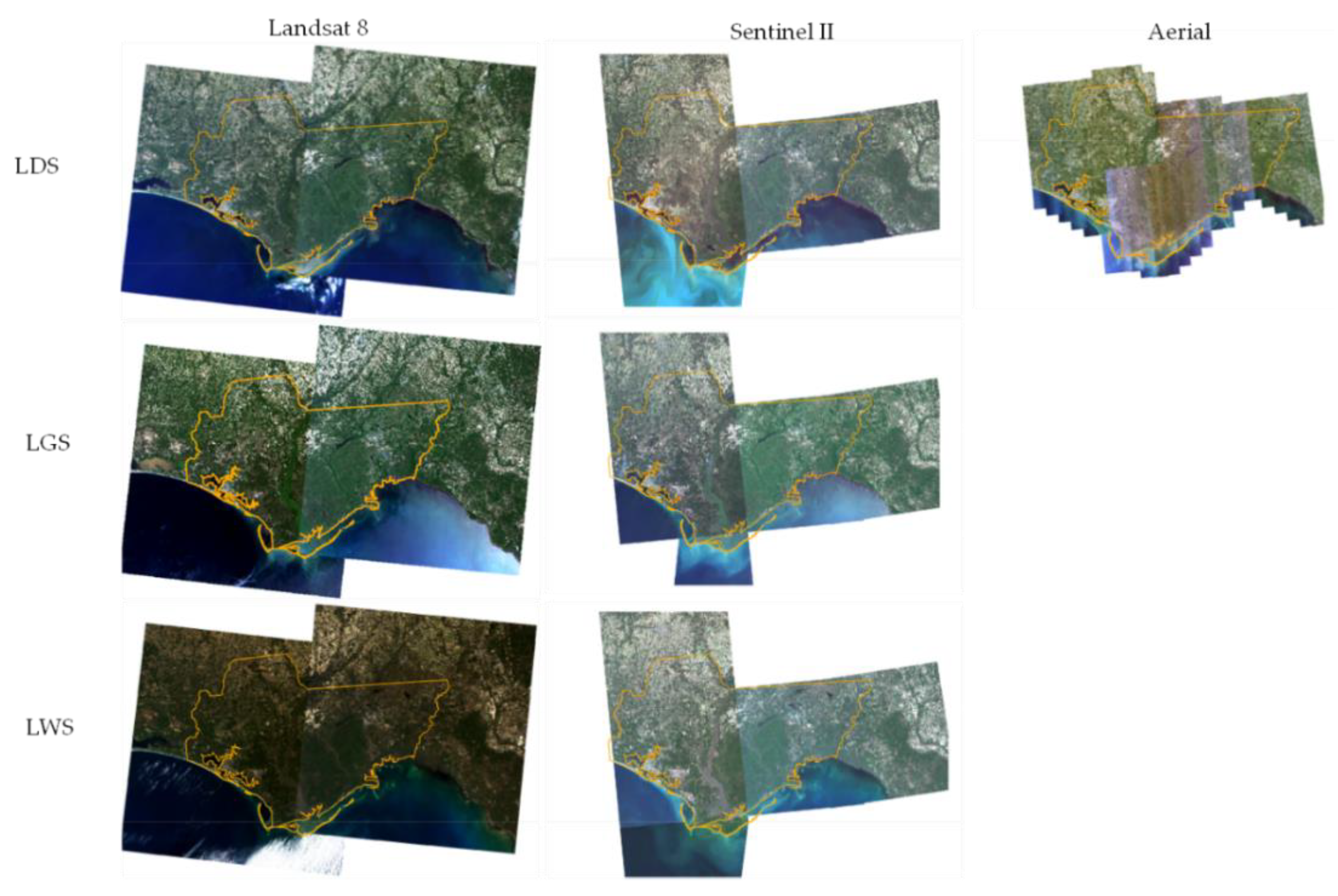
2.5. Image Normalization

Remotely sensed data were re-scaled to a common radiometric scale using an enhanced aggregate no-change regression (EANR) methodology. Similar to aggregate no-change regression (ANR) [6,23], EANR seeks to leverage strong linear relationships among Landsat, Sentinel 2, and aerial image bands to bring finer spatial resolution imagery to the same relative radiometric scale as coarser imagery. The main differences between EANR and ANR are: (1) an added aggregation step to bring finer resolution imagery to the same spatial scale as the reference imagery, (2) a normalization of raw digital number (DN) values, (3) a trimming procedure to mitigate confounding effects of land use/cover changes for images acquired at different dates, and (4) a sampling scheme to extract spectral aggregates within overlapping image boundaries.

Like ANR, EANR extends the concepts of automatic scattergram-controlled regression [24] by applying an area slicing algorithm to identify no-change pixels. It then spatially aggregates pixel values around selected locations to minimize the effect of co-registration errors [20,23]. Aggregated values at selected locations of the subject image are then regressed against the corresponding values for a reference image using ordinary least squares regression (OLS) on a band-by-band basis. Finally, regression coefficients are applied to the subject image to bring it to the same radiometric scale as the reference image and to other fine-scaled images that overlap the same reference image.

Critical to this process is the elimination of areas and pixels within the region of image overlap that have been affected by land use or land cover change. This was accomplished in two steps. The first step required visually estimating the proportion (p_Δ) of area within the overlapping regions of the images that were impacted by changes due to phenomena such as clouds, land use change, or land cover change. For our study, we used an estimate of p_Δ = 20 percent to mask Landsat 8 and Sentinel 2 pixels. For aerial imagery we used a p_Δ ranging between 20 and 30 percent. Applying these change proportions, raw DN values were separately normalized $\left(\widehat{DN}\right)$ to the unit scale for each of the subject (S) and reference (R) images and bands (k). Differences in the normalized $\widehat{DN}$ values between subject and reference images were then obtained for each band:

$$\mathsf{\Delta }{\widehat{DN}}_k={\widehat{DN}}_{R_k}-{\widehat{DN}}_{S_k}$$

(1)

For step two, the $\mathsf{\Delta }{\widehat{DN}}_k$ values were ordered from smallest to largest. Pixels in the lower 10% (i.e., 0.5p_Δ) and upper 10% were identified as “change” pixels and masked from subsequent analyses.

The spatial aggregation process minimizes the effect of co-registration errors [20] by extracting and calculating the mean values of unchanged pixels within the overlap of each image at a coarser grain size. In this procedure an aggregation block window size of 270 m by 270 m was chosen based on simulated results found for Landsat 8 co-registration errors reported in Hogland and Affleck [20]. Aggregated blocks with more than 30 percent of the pixels identified as no-change were used for regression analyses of subject image blocks on reference image blocks for individual bands. The resulting regression coefficients for each band were then applied back to the non-aggregated pixel values of the subject image. The described EANR procedure was developed and integrated into the RMRS Raster Utility project [22] (Supplemental Materials 2).

For Landsat 8 and Sentinel 2 images, we used EANR with 1000 randomly chosen locations within regions of overlap to bring images within a given season to a common relative radiometric scale. For normalization of Landsat 8 imagery, path/row 18/39 data were used as the reference images for each season. Reference images for normalization of Sentinel 2 imagery are specified in Table A2. For aerial imagery, normalized Landsat 8 imagery was used as the reference image. In instances when substantial land use or land cover change had occurred due to differences in image acquisition dates (e.g., changes in agricultural fields), manually defined spatial masks were used to remove additional pixels prior to implementation of the EANR procedure (Figure 3).

2.6. Spectral and Texture Metrics

Once normalized, focal mean and standard deviation analyses [5,6,22] were performed to quantify texture and mimic field plot extents for each band, season, and source of remotely sensed imagery (

Table 2. Sources, spatial resolution, and labeling of imagery used in comparisons.

Source	Code	Resolution	Bands	Spectral and Texture Metrics	Season	ID
Landsat 8	L	30 m	2–7	Mean (Cell)	LDS	1–6
					LGS	7–12
					LWS	13–18
				Standard Deviation (3 by 3 Cells)	LDS	19–24
					LGS	25–30
					LWS	31–36
Sentinel 2	S	10 m	2, 3, 4, and 8	Mean (3 by 3 Cells)	LDS	1–4
					LGS	5–8
					LWS	9–12
				Standard Deviation (5 by 5 Cells)	LDS	13–16
					LGS	17–20
					LWS	21–24
Quantum Spatial	A	0.6 m	1–4	Mean (61 by 61 Cells)	LDS	1–4
				Standard deviation (61 by 61 Cells)	LDS	5–8

). Due to differing spatial resolutions of the imagery, various window sizes were used to capture spectral and texture patterns at approximately the same spatial resolution as the field plot extent. Window sizes for each image source were chosen based on the smallest window extent with an odd number of rows and columns that could be used to calculate focal mean and standard deviation statistics without resampling the imagery. For Landsat 8 imagery, mean band DN values were extracted based on the location of a given field plot and the nearest pixel (30 m by 30 m spatial resolution). Additionally, at those locations, Landsat 8 band standard deviations for a three by three moving window (90 m by 90 m) were calculated for each pixel and extracted. For Sentinel 2 imagery, a three by three moving window (30 m by 30 m) was used to calculate mean values and a five by five window (50 m by 50 m) was used to calculate standard deviation. For aerial imagery, a 61 by 61 window (grain size of 0.6 m, ~37 m by 37 m) was used to calculate image mean and standard deviation at each location. In total, 68 different metrics were created and extracted from the normalized remotely sensed imagery using the averaged GPS location of each field plot and the nearest image pixel. As shown in Table 2, these metrics include 36 band values extracted from Landsat 8 based imagery (2 metrics for 6 bands and 3 seasons), 24 band values extracted from Sentinel 2 based imagery (2 metrics for 4 bands and 3 seasons), and 8 band values extracted from the aerial imagery (2 metrics for 4 bands and 1 season). To evaluate the impact of EANR on estimating DFT, LLP, BAH and TPH, this metric creation and extraction process was repeated for non-normalized imagery and the values from both sets were used to build and compare models.

2.7. Model Development, Comparisons, and Raster Surface Creation

For each response variable (DFT and LLP classes, plus Pine and Other tree species BAH and TPH) we used a variable selection routine described in [5,6] to select EANR normalized and non-normalized remotely sensed metrics that significantly (α = 0.05) improved the model fit of generalized additive models (GAMs), as defined by increased percent deviance explained. This variable selection routine uses GAMs, deviance, and pseudo p-values to iterate through potential predictor variables and exhaustively find the combination of additive variables that are both significant and improve the model fit by a user specified amount (Supplemental Materials 3). GAMs are a flexible modeling technique that can accommodate nonlinear relationships between response and predictor variables using penalized regression splines [25] and can be applied to non-Gaussian response data such as the DFT and LLP. While useful in identifying nonlinear, nonparametric relationships, GAMs can overfit sample data making estimates less generalizable to a given population [26]. To address the issue of overfitting, we employed a Monte Carlo re-sampling scheme to build a suite of 50 GAMs constructed from random subsets of our data. For each of the 50 GAMs, 75 percent of the observations within our sample were used to develop relationships between a given response and our previously selected predictor variables. The remaining 25 percent of the observations that were not used to build the GAM constituted an out of bag (OOB) subset of the data and were used to assess the accuracy of GAM estimates $\left(\widehat{P}\right)$. Statistics calculated for assessment were root mean squared error (RMSE) for continuous response variables (BAH and TPH) and classification accuracy (from a most likely class rule) for the binomial (LPP) and multinomial (DFT) categorical response variables. Once calibrated, we applied the ensemble of 50 GAMs (EGAM) to estimate each response variable $\left(\widehat{E}\right)$ and corresponding standard error $\left(\widehat{SE}\right)$ at the pixel level as follows:

$$\widehat{E}=\frac{1}{n}{\displaystyle \sum }_{i=1}^n{\widehat{P}}_i\hspace{1em}and\hspace{1em}\widehat{SE}=\sqrt{\frac{1}{n}{\displaystyle \sum }_{i=1}^n{\left({\widehat{P}}_i-\widehat{E}\right)}^2}$$

(2)

EGAMs based on EANR normalized imagery were compared against EGAMs based on non-normalized imagery using averaged RMSE, classification accuracy statistics, and Akaike’s information criterion (AIC) [27,28]. Our best fitting EGAMs (normalized versus raw image based predictors) were used with the corresponding image metrics to produce raster surfaces depicting the condition of forests in the ASGA. Additionally, estimation errors at field plot locations were evaluated for spatial correlation using a global Moran’s I test [29]. The described analyses and procedures were developed and performed in R statistical software [30] and are available in Supplemental Materials 3.

3. Results

3.1. Field Data

Plot summaries from field data are displayed in Figure 4 and Table 1. Almost half the plots were in the Pine class (48%), but only 16.8% contained longleaf pine trees above 5 cm dbh and BAH above 2 m² ha⁻¹. Mean BAH for the DFT Other class was only slightly higher than that for the DFT Pine class, but BAH was more variable in the former. Mean TPH and variability in TPH was substantially lower in the Pine class relative to the Other forested class. Taken together, this indicates that tree diameter (dbh) tended to be larger in the Pine class.

3.2. Image Normalization

The EANR-adjusted Landsat 8, Sentinel 2, and aerial imagery is shown in Figure 5. The R² statistics for LDS, LGS, and LWS Landsat 8 normalization regressions were generally large (greater than 0.9; Figure 6) across all bands, with the lowest R² coinciding with LWS analyses. Similarly, for Sentinel 2 imagery, the R² statistics of the image-to-image overlap regressions were large (greater than 0.9) with the lowest occurring in LWS. The strength of these associations resulted in the improved radiometric consistency across Landsat 8 and Sentinel 2 images that is visually evident in Figure 5 (cf. Figure A1). In contrast, regressions of overlapping aerial and Landsat 8 Imagery were weak for several flight paths (Figure 6). The acquisition dates for these paths tended to be later (Figure 3) and potentially coincided with substantial changes in plant phenology. As a result, original scene boundaries were still apparent in normalized aerial image mosaics (Figure 5).

3.3. Sample Distribution

Clusters derived from spectral and texture metrics using the k-means unsupervised clustering algorithm divided the feature space into 100 classes of varying size (Figure 7). The distribution of the field plot locations across those same 100 classes shows that the field plots spanned a wide range of the feature space, but did not capture all the spectral classes. Many of the classes not represented at field plot locations corresponded to urban and agricultural cover types.

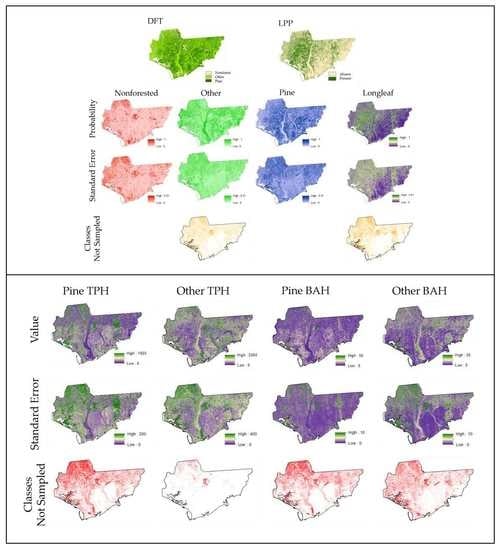
3.4. Model Development, Comparisons, and Raster Surface Creation

Spectral and texture metrics selected for modeling varied by response variable and whether images were normalized to a common radiometric scale (

Table 3. Selected predictor variables and mean error statistics for normalized (EANR) and non-normalized (RAW) based ensemble generalized additive models (EGAMs). Error statistics for dominant forest type (DFT) and longleaf pine presence (LPP) models are in terms of 1–accuracy of the classification, while BAH and TPH errors are measured in terms of root mean squared error (RMSE) on the square root scale. Train and out of bag (OOB) errors denote whether error statistics were calculated from observations used to train a given model or withheld from training, respectively. Mean Akaike information criterion ($\overline{\mathrm{AIC}}$) was calculated using training data and the AIC statistics for each generalized additive model within the corresponding ensemble.

Response	Normalization	Predictors *	Train	OOB	AIC
DFT	EANR	L3, L16, L17, S2, S5, S7, S21, A1	0.068	0.235	86.217
	RAW	L8, L9, L16, L18, S11, S5	0.103	0.263	110.023
LPP	EANR	L2, L17, S3, S4, A2, A5	0.056	0.129	94.683
	RAW	L2, L13, S9, A6	0.095	0.148	113.617
$\sqrt{\mathrm{Pine}\mathrm{BAH}}$	EANR	L2, L8, L10, L11, L16, L17, L18, L22, A2, A8	0.909	1.168	548.664
	RAW	L2, L5, L6, L8, L10, L11, L17, L22, S9, S10, S11, S12, A4	0.900	1.267	547.441
$\sqrt{\mathrm{Other}\mathrm{BAH}}$	EANR	L3, L5, L11, S7, S9, S21, S23, A2, A5	1.108	1.365	600.177
	RAW	L3, L5, L11, L13, L16, S12, A5, A7	1.188	1.541	637.448
$\sqrt{\mathrm{Pine}\mathrm{TPH}}$	EANR	L3, L5, L8, L10, L11, L17, L28, S4, S11, A2, A5	5.755	9.197	1243.537
	RAW	L1, L4, L5, l6, L13, L22, L31, S11, S20	6.709	10.866	1277.418
$\sqrt{\mathrm{Other}\mathrm{TPH}}$	EANR	L9, L13, S2, S6, S7, S20, A1	11.787	14.977	1471.036
	RAW	L3, L5, L11, L13, S12, S20, A5	12.492	14.682	1486.281

* Predictor variable naming convention is based on the concatenation of Table 1 Code and Id columns.

). Using the variable selection procedure described by Hogland et al. [6], EGAMs selected between four and twelve metrics out of the potential 68, at a significance threshold of α = 0.05. In all instances, metrics were selected from each image source and from multiple seasons (Table 2 and Table 3). Compared with EGAMs built using non-normalized texture metrics, EANR based EGAMs generally improved model fit as measured by average classification error, RMSE, and AIC (Table 3). EGAMs based on non-normalized imagery generally selected fewer metrics and tended to utilize metrics derived from Landsat 8 and Sentinel 2 data sources. In all cases, EGAMs that used normalized predictors were selected as the top fitting models and used to assess accuracy and create raster surfaces.

Overall classification accuracies for top fitting DFT and LPP EGAMs were greater than 88% with the most common classification errors being the mapping of the Other forested class as pine, and longleaf presence being mapped as absence (Figure 8). Training and OOB errors for DFT, LPP, BAH and TPH EGAMs are reported in Table 3 and suggest strong relationships among response and normalized predictor variables, particularly in the Pine class. Estimated BAH and TPH values from top fitting models were also strongly correlated with observed values, though in densely stocked conditions (TPH above 1000 stems ha⁻¹, BAH above 20–30 m² ha⁻¹), EGAMs tended to underestimate BAH and TPH (Figure 9). Estimation errors for some EGAMs were positively spatially correlated, suggesting spatial patterns or trends in model errors (

Table 4. Global Moran’s I (GMI) statistics and p-values for the hypothesis of no spatial association for ensemble generalized additive model (EGAM) residuals.

EGAM *	GMI	p-Value
DFT (Nonforest)	0.364	<0.001
DFT (Other)	0.067	0.190
DFT (Pine)	0.093	0.153
LPP (Present)	0.223	0.002
Pine BAH	0.184	0.011
Pine TPH	0.068	0.188
Other BAH	0.087	0.131
Other TPH	0.140	0.037

* DFT = dominant forest type, LPP = longleaf pine presence, BAH = basal area per ha (m²), TPH = trees per ha.

). Though tempting to address the spatial variability in estimation error using kriging [31], our sample design does not lend itself to accounting for spatial trends in the residuals across the largely privately-owned tracts of the AGSA that were outside the target population.

EGAM raster surfaces were created at a spatial resolution of 30 m across the ASGA for all response variables. For DFT and LPP, EGAM estimates include class probabilities and model-based estimated standard errors for each cell within the study area. For pine and other $\sqrt{BAH}$ and $\sqrt{TPH}$, estimates and standard errors were calculated using squared transformations of EGAM estimates.

DFT and LPP raster surfaces are presented in Figure 10 while BAH and TPH surfaces are presented in Figure 11. Additionally, Figure 10 and Figure 11 display the spatial distribution of EGAM-specific feature space k-means classes that were not represented within the sample. Some banding of estimates and standard errors is evident in Figure 10 and Figure 11 for the models using the A2 and A5 metrics (e.g., for LLP, Pine TPH, Other BAH) in the eastern portion of the ASGA. Those bands tend to appear in the corresponding sample representation maps, suggesting that certain flight paths in the aerial imagery could not be fully normalized and were unable to be adequately sampled in the field.

4. Discussion

We mapped key forest characteristics across ASGA that can be used to inform spatially explicit longleaf restoration decision making. These surfaces transform data that are relatively easy to collect into pertinent information for longleaf pine restoration, providing the fine level of spatial detail and accuracy needed to make well-informed restoration decisions. We have also described a procedure for, and demonstrated the importance of, bringing images to a common radiometric scale across sources, years, and spatial resolutions (Figure 5). Models built with EANR-normalized spectral and texture metrics utilized distinct sources, phenological seasons, and bands, and had less error than models built using the raw imagery (Table 3). Additionally, our study highlights how multiple image resolutions (temporal, spectral, and spatial) can improve model fit and estimation, especially after images have been brought to a common radiometric scale using a technique like EANR. Finally, we presented and implemented an EGAM approach to estimate DFT, LPP, and BAH and TPH for pine and other tree species groups that accommodates nonlinear relationships while mitigating the potential for overfitting. Combined, EANR and EGAM produce better estimates of key forest characteristics than previous longleaf pine mapping efforts [5,6] (reductions in classification error and RMSE). Moreover, the EGAM procedure provided spatial depictions of estimation error (standard error surfaces) that can be used by resource managers when making management decisions.

Sample design played an important role in our study. Because some areas were inaccessible, field sampling was limited to a subset of the ASGA (Figure 2). This limitation means that inferences must rely on the assumptions that the sample adequately characterizes the feature space and that the predictor–response relationships do not vary among different ownership types across the ASGA. For our study, the sampled locations captured an appreciable extent of the feature space (Figure 7, Figure 10 and Figure 11) and there were relatively strong relationships among response and predictor variables. Because of these reasons we feel relatively confident that the model estimates provide an accurate depiction of forested conditions across the ASGA. However, our assessment did identify portions of the feature space that were unsampled, and others that were over- or under-represented. From a model calibration perspective, overrepresentation can be thought of as wasted effort when variability in the predictor–response relationship is relatively minor. In those instances, observations from overrepresented regions of feature space could potentially be reallocated to unsampled or underrepresented areas. Additionally, our assessment detected some geographic areas where the imagery could not be adequately normalized and thus may have related differently to the vegetation conditions. Future designs should attempt to spread sample locations across predictor variable space, while balancing the sample to mimic the distributional characteristics of the population [32]. Toward this end, the raster surfaces created from this study could be used to spread and balance sampling locations for future studies [33], thereby providing additional means to minimize error and reduce sample cost.

Quantitatively, DFT and LPP EGAM fit statistics suggest that our models accurately depicted forest cover types and the presence of longleaf pine. Similarly BAH and TPH EGAM estimates were strongly correlated with observed plot BAH and TPH over the more commonly observed lower ranges of these variables. Moreover, EANR based EGAMs outperformed EGAMs based on spectral and texture metrics from raw imagery. Interestingly, the correlation between observed and predicted values for Other TPH was substantially less than BAH and Pine TPH models, especially when tree densities were high. This may be due to the variability in tree crown shapes associated with the various tree species of the Other class (Table A1). However, further investigation is needed to substantiate this claim.

Qualitatively, our raster surfaces display more detail and are less impacted by variation in image acquisition dates when compared to previous mapping efforts [5]. However, there were instances when our EGAMs appeared to underestimate TPH (Figure 9) and to omit instances when longleaf pine was present (Figure 8). For example, when TPH was greater than 1000 ha⁻¹ (e.g., as would be the case in young or overstocked stands), EGAMs underestimated TPH. Additionally, some areas dominated by cities, agricultural fields, water, and aquatic vegetation were underrepresented or not represented (Figure 10 and Figure 11) in our sample and led to imprecise estimates (Figure 12). However, DFT, LPP, BAH and TPH models generally produced reliable, spatially explicit estimates.

While estimation error could be reduced for almost every EGAM by including additional EANR normalized spectral and texture predictive variables (i.e., setting an α = 0.1), the added complexity and processing associated with including more variables outweighed the marginal gains in accuracy. Similarly, many of the predictor variables used in our EGAMs were highly correlated, suggesting marginal utility of additional metrics. Additionally, areas within feature space that were underrepresented or not represented generally produced extremely variable estimates, which should be viewed with skepticism. Moreover, EGAMs that were more complex (i.e., more predictor variables) tended to have larger proportions of the expanded feature space underrepresented. This suggests that for limited sample sizes, simpler models (i.e., fewer predictors) may be preferred for wall to wall mapping endeavors along with masking land cover types that are not forested. Finally, for some of our EGAMs, estimation errors exhibited minor positive spatial correlation. While tempting to use kriging methods [31] to remove global spatial trends in estimation error, our design did not adequately sample geographic space across ASGA, limiting the utility of kriging methods to contiguous accessible areas sampled within our study.

Though additional improvements can be made to our estimates of forest characteristics, tradeoffs between processing, model development, and sampling costs related to improvements in accuracy should be weighed to evaluate the level of precision needed to inform decision making [34]. Given the amount of model error potentially introduced by co-registration errors [20], our EGAMs explained the majority of the variation that can be accounted for within the field data and provide a substantial improvement over previous efforts [5,6]. Additionally, by implementing an ensemble approach to generalized additive models, we were able to capture nonparametric trends in the data while mitigating overfitting and providing a technique to empirically estimate model-based standard errors. The resultant estimates and standard errors provide the type of information needed to make both fine and coarse grained restoration decisions across the ASGA.

For example, DFT, LLP, Pine and Other BAH and TPH, and standard error raster surfaces, can be combined using a geographic information system and map algebra to locate, prioritize, and quantify overstocked pine areas where longleaf pine trees are present. The resulting surfaces from those spatial analyses can then be used to plan thinning and prescribed fire regimes to restore those areas to healthy longleaf ecosystem stand densities and compositions [35]. Similarly, these same surfaces could be used to locate, prioritize, and quantify areas where tree species other than pine make up the dominant component of BAH (DFT Other class) but still have a remnant pine and longleaf element (hardwood encroachment). Once identified, silviculture prescriptions can be planned and implemented to convert those locations into a healthy longleaf ecosystem. Moreover, those silviculture prescriptions can be designed in such a manner that they can be spatially depicted and coupled with BAH and TPH surfaces and logistic spatial modeling techniques as described in [36] to quantify implementation costs and further prioritize these types of restoration efforts.

5. Conclusions

Adept forest management requires accurate information concerning the status and distribution of forest resources. To create accurate information pertinent to longleaf pine restoration, we developed procedures to bring multi-temporal images to a common radiometric scale, model nonparametric relationships between remotely sensed and field measured data, and produce spatial depictions of forest cover types, longleaf pine presence, and BAH and TPH by forest cover class. These procedures and sources of data were combined to produce the types of information needed to inform longleaf restoration planning and implementation at planning and tactical spatial scales across a relatively large area in northwestern Florida.

References

1. Noss, R.; LaRoe, E.; Scott, J. Endangered Ecosystems of the United States: A Preliminary Assessment of Loss and Degradation; Biological Report 28; National Biological Service: Washington, DC, USA, 1995; Available online: https://sciences.ucf.edu/biology/king/wp-content/uploads/sites/106/2011/08/Noss-et-al-1995.pdf (accessed on 19 July 2019).
2. Oswalt, C.; Cooper, J.; Brockway, D.; Brooks, H.; Walker, J.; Connor, K.; Oswalt, S.; Conner, R. History and Current Condition of Longleaf Pine in the Southern United States; USDA Forest Service General Technical Report SRS-166; United States Forest Service: Ashville, NC, USA, 2012. Available online: http://www.srs.fs.usda.gov/pubs/42259 (accessed on 6 February 2019).
3. Regional Working Group for America’s Longleaf. Range-Wide Conservation Plan for Longleaf. 2009. Available online: http://www.americaslongleaf.org/media/86/conservation_plan.pdf (accessed on 6 February 2019).
4. U.S. Forest Service Forest Inventory and Analysis Program: We Are the Nation’s Forest Census. Available online: https://www.fia.fs.fed.us/ (accessed on 6 February 2019).
5. Hogland, J.; Anderson, N.; St. Peter, J.; Drake, J.; Medley, P. Mapping forest characteristics at fine resolution across large landscapes of the southeastern United States using NAIP imagery and FIA field plot data. ISPRS Int. J. Geo-Inf. 2018, 7, 140. Available online: https://www.mdpi.com/2220-9964/7/4/140/htm (accessed on 6 February 2019). [CrossRef] [Green Version]
6. Hogland, J.; Anderson, N.; Affleck, D.L.R.; St. Peter, J. Using Forest Inventory Data with Landsat 8 imagery to Map Longleaf Pine Forest Characteristics in Georgia, USA. Remote Sens. 2019, 11, 1803. [Google Scholar] [CrossRef] [Green Version]
7. Gibert, K.; Horsburgh, J.S.; Athanasiadis, I.N.; Holmes, G. Environmental Data Science. Environ. Model. Softw. 2018, 106, 4–12. [Google Scholar] [CrossRef]
8. Homer, C.; Dewitz, J.; Yang, L.; Jin, S.; Danielson, P.; Xian, G.; Coulston, J.; Herold, N.; Wickham, J.; Megown, K. Completion of the 2011 National Land Cover Database for the conterminous United States-Representing a decade of land cover change information. Photogr. Eng. Remote Sens. 2015, 81, 345–354. [Google Scholar]
9. LANDFIRE. Existing Vegetation Type Layer, LANDFIRE 1.1.0, U.S. Department of the Interior, Geological Survey. 2008. Available online: http://landfire.cr.usgs.gov/viewer/ (accessed on 28 October 2010).
10. Brunner, R.J.; Kim, E. Teaching Data Science. Procedia Comput. Sci. 2016, 80, 1947–1956. [Google Scholar] [CrossRef] [Green Version]
11. Lokers, R.; Knapen, R.; Janssen, S.; van Randen, Y.; Jansen, J. Analysis of Big Data technologies for use in agro-environmental science. Environ. Model. Softw. 2016, 84, 494–504. [Google Scholar] [CrossRef] [Green Version]
12. The Longleaf Alliance. About ARSA. Available online: https://www.longleafalliance.org/arsa/about-arsa (accessed on 23 October 2019).
13. Quantum Spatial. About Use. Available online: https://www.quantumspatial.com/about-us (accessed on 23 October 2019).
14. Earth Observing System [EOS]. Sentinel-2. Available online: https://eos.com/sentinel-2/ (accessed on 23 October 2019).
15. United States Geological Survey [USGS]. Landsat 8. Available online: https://www.usgs.gov/land-resources/nli/landsat/landsat-8?qt-science_support_page_related_con=0#qt-science_support_page_related_con (accessed on 23 October 2019).
16. USGS. Landsat 8 Surface Reflectance Code (LASRC) Product Guide. General Technical Report LSDS-1368 Version 2.0. 2019. Available online: https://prd-wret.s3-us-west-2.amazonaws.com/assets/palladium/production/atoms/files/LSDS-1368_L8_Surface_Reflectance_Code_LASRC_Product_Guide-v2.0.pdf (accessed on 19 July 2019).
17. Florida Natural Areas Inventory [FNAI]. About Us. Available online: https://www.fnai.org/about.cfm (accessed on 23 October 2019).
18. ESA Sentinel Online. Copernicus Open Access Hub. Available online: https://scihub.copernicus.eu/dhus/#/home (accessed on 23 October 2019).
19. USGS. EarthExplorer—Home. Available online: https://earthexplorer.usgs.gov/ (accessed on 23 October 2019).
20. Hogland, J.; Affleck, D.L.R. Mitigating the Impact of Field and image Registration Errors through Spatial Aggregation. Remote Sens. 2019, 11, 222. [Google Scholar] [CrossRef] [Green Version]
21. Souza, C. Accord.Net Framework. Available online: http://accord-framework.net/ (accessed on 27 September 2013).
22. Hogland, J.; Anderson, N. Function Modeling Improves the Efficiency of Spatial Modeling Using Big Data from Remote Sensing. Big Data Cogn. Comput. 2017, 1, 3. [Google Scholar] [CrossRef] [Green Version]
23. Hogland, J. Creating Spatial Probability Distributions for Longleaf Pine Ecosystems Across East Mississippi, Alabama, The Panhandle of Florida, and West Georgia, Thesis. 2005. Available online: https://etd.auburn.edu/bitstream/handle/10415/603/HOGLAND_JOHN_19.pdf?sequence=1&isAllowed=y (accessed on 20 December 2017).
24. Elvidge, C.D.; Yuan, D.; Weerackoon, R.D.; Lunneta, R.S. Relative radiometric normalization of Landsat Multispectral Scanner (MSS) data using an automatic scattergram-controlled regression. Photogramm. Eng. Remote Sens. 1995, 61, 1255–1260. [Google Scholar]
25. Wood, S.N. Fast stable restricted maximum likelihood and marginal likelihood estimation of semiparametric generalized linear models. J. R. Stat. Soc. 2011, 73, 3–36. [Google Scholar] [CrossRef] [Green Version]
26. Wood, S.N.; Augustin, N.H. GAMs with integrated model selection using penalized regression splines and applications to environmental modeling. Ecol. Model. 2002, 157, 157–177. [Google Scholar] [CrossRef] [Green Version]
27. Akaike, H. Information theory and an extension of the maximum likelihood principle. In Proceedings of the 2nd International Symposium on Information Theory, Tsahkadsor, Armenia, 2–8 September 1971; Petrov, B.N., Csaki, F., Eds.; Akadémiai Kiadó: Budapest, Hungary, 1973; pp. 267–281. [Google Scholar]
28. Akaike, H. A new look at the statistical model identification. IEEE Trans. Autom. Control 1974, 19, 716–723. [Google Scholar] [CrossRef]
29. Moran, P. Notes on Continuous Stochastic Phenomena. Biometrika 1950, 37, 17–23. [Google Scholar] [CrossRef] [PubMed]
30. R Core Team. R: A Language and Environment for Statistical Computing; R Foundation for statistical Computing: Vienna, Austria, 2014; Available online: http://www.R-project.org/ (accessed on 28 April 2018).
31. Cressie, N.A.C. Statistics for Spatial Data, Revised ed.; John Wiley & Sons, Inc.: Hoboken, NJ, USA, 1993; p. 928. [Google Scholar]
32. Tille, Y.; Wilhelm, M. Probability Sampling Designs: Principles for Choice of Design and Balancing. Stat. Sci. 2017, 32, 176–189. [Google Scholar] [CrossRef] [Green Version]
33. Gregoire, T.; Valentine, H. Sampling Strategies for Natural Resources and the Environment; Chapman & Hall: Boca Raton, FL, USA; London, UK; New York, NY, USA, 2008; 474p. [Google Scholar]
34. Ruotsalainen, R.; Pukkala, T.; Kangas, A.; Vauhkonen, J.; Tuaominen, S. The effects of sample plot selection strategy and the number of sample plots on inoptimality losses in forest management planning based on airborne laser scanning data. Can. J. For. Res. 2019, 49, 1135–1146. [Google Scholar] [CrossRef]
35. Hogland, J.; Anderson, N.; Chung, W. New Geospatial Approaches for Efficiently Mapping Forest Biomass Logistics at High Resolution over Large Areas. ISPRS Int. J. Geo-Inf. 2018, 7, 156. [Google Scholar] [CrossRef] [Green Version]
36. America’s Longleaf. Longleaf Pine Maintenance Condition Class Definitions. Available online: http://www.americaslongleaf.org/media/mjroaokz/final-lpc-maintenance-condition-class-metrics-oct-2014-high-res.pdf (accessed on 2 April 2020).
37. U.S. Forest Service; Forest Inventory and Analysis (FIA). Database, U.S. Department of Agriculture, Forest Service; Northern Research Station: Saint Paul, MN, USA, 2019. Available online: https://apps.fs.usda.gov/fia/datamart/datamart.html (accessed on 6 February 2019).
Figure 1. Apalachicola Significant Geographic Area (ASGA) location map (right) and image boundaries (left). Landsat 8 and Sentinel 2 images were acquired for three seasons, representing a leaf on growing season (LGS), leaf on dormant season (LDS), and a leaf off winter season (LWS). Aerial imagery was only acquired for LDS. Image acquisition dates can be found in Table A2.
Forests 11 00426 g001
Figure 2. Spatial allocation (left) and layout (right) of field plots overlaid on aerial imagery. Target population (tan colored region) accounted for approximately 23% of the total area within the ASGA.
Forests 11 00426 g002
Figure 3. Example of spatial masks (semitransparent beige polygon with green border) and random locations (yellow points) used in the enhanced aggregate no-change regression procedure (EANR) for LDS Landsat 8, Sentinel 2, and aerial imagery. Light blue polygons highlight the overlapping area between images acquired at different dates while masked areas highlight a subset of that area composed primarily of forest vegetation.
Forests 11 00426 g003
Figure 4. Histograms and summary statistics of plot basal area m2 ha−1 (BAH) and trees ha−1 (TPH) for pine and other tree species groups.
Forests 11 00426 g004
Figure 5. Landsat 8, Sentinel 2, and Aerial true color mosaics for leaf on fall dormant (LDS), leaf on spring growing (LGS), and leaf off winter (LWS) seasons following EANR radiometric scaling. The AGSA boundary is outlined in orange.
Forests 11 00426 g005
Figure 6. Box plots of enhanced aggregate no-change normalization (EANR) coefficients of determination (R2) results for each source of imagery and season across all image bands. For Landsat 8 and Sentinel 2, the reference and subject images were of the same source; for Aerial analyses, the reference images were normalized Landsat 8 imagery.
Forests 11 00426 g006
Figure 7. Estimated proportion of AGSA (orange) falling within each of 100 classes derived from an unsupervised classification of normalized Landsat 8, Sentinel 2, and aerial imagery, plus the proportion of 244 field plots (blue) within those same classes.
Forests 11 00426 g007
Figure 8. Accuracy assessment for dominant forest type (DFT) and presence of longleaf pine (LPP) using all 244 field plots and the corresponding ensemble generalized additive model (EGAM). Exact 95 percent lower and upper confidence limits for each class are reported above and below bold numbers within the error matrix and within parentheses of overall accuracy.
Forests 11 00426 g008
Figure 9. Predicted versus observed values (blue circles) of basal area per ha (BAH) and trees per ha (TPH) for pine and other tree species groups derived from ensemble generalized additive models (EGAMs) that used normalized predictors. The black dashed line shows the general trend based on a loess smooth estimator with grey shaded 95 percent confidence bands. The red line denotes a one to one line.
Forests 11 00426 g009
Figure 10. Spatial distribution of the dominant forest type most likely class (DFT), class probabilities, and class probability standard errors for Nonforested (red), Other (green), and Pine (blue) cover types (Table 1). Additionally, presence and absence of longleaf pine within a plot based on a most likely class rule (LPP), presence probabilities, and presence probability standard errors (purple to green color gradient). Finally, the spatial location of k-mean classes not represented in the sample used to train EGAMs are displayed as orange areas in the bottom row of graphics.
Forests 11 00426 g010
Figure 11. Display of trees per ha (TPH) and basal area per ha (BAH) raster surfaces created from ensemble generalized additive models (EGAMs) for Pine and Other tree species classes. EGAM raster cell estimated values (top row of graphics) and standard errors (middle row of graphics) increase as colors transition from purple to green. The spatial locations of k-mean classes not represented in the sample used to train EGAMs are displayed as red areas in the bottom row of graphics.
Forests 11 00426 g011
Figure 12. A close up example of locations with large standard errors in estimated Pine BAH owing to underrepresentation of feature space classes within the sample.
Forests 11 00426 g012