Analyzing Potential Tree-Planting Sites and Tree Coverage in Mexico City Using Satellite Imagery

Abstract

Locating potential tree-planting sites and analyzing tree canopy cover is important in the planning and management of urban forests. This paper reports the quantification of potential planting sites as well as tree canopy cover in the urban area of Mexico City, estimated by means of SPOT (Satellite Pour l’Observation de la Terre) 6 satellite images and a supervised pixel-based classification approach. Results showed an estimated area of 3100.7 ha of potentially useful sites, including places with bare soil and grass-covered areas such as median strips, roundabouts and parks. An average tree canopy cover of 10.6% and an average impervious surface of 79.2% for the 15 boroughs were also analyzed. The area of potential planting sites would represent a 5% gain for the current tree canopy cover if it were to be planted. With an overall accuracy of 92.4%, the use of both images from the SPOT 6 sensor and the classification approach proved to be appropriate for obtaining thematic covers in the urban environment of Mexico City.

1. Introduction

Spaces with vegetation play a critical role in the proper functioning of cities, impacting the quality of life of their inhabitants. Trees are the most essential elements of such spaces as the primary providers of a wide range of environmental services [1,2,3,4,5,6]. Increasing tree cover is thus one of the most cost-effective strategies for reducing the various adverse effects of urbanization, such as heat islands, excessive consumption of electricity for heating and cooling buildings, and daily stress [7,8,9,10,11].

Quantifying the tree canopy cover (TCC)—a canopy-occupied area viewed from above—of a city assists in planning, managing, and researching the present vegetation, as well as in estimating the value of the services by revealing both the characteristics and distribution of the trees [12,13]. Knowledge of tree canopy cover and potential planting sites is important in increasing the size of urban forests. Today, urban planners and decision-makers require this detailed information to guide the selection and maintenance of trees appropriate to the local conditions of the site [14], since in most cases complete information regarding the urban forest, the community framework and a resource management approach is lacking [12,15].

Traditionally, this information is generated through the interpretation of aerial photographs or field inventories, resulting in a considerable expenditure of time and the need for trained personnel. In addition to being slow, neither method provides complete coverage of large areas [16,17,18,19]. Nowadays, the availability of multiple sources of images from remote sensing and different processing techniques allows urban specialists to evaluate the TCC more efficiently, with the advantage of obtaining information on a large area in less time and with increasing precision [14,20,21,22,23,24].

Remote sensing techniques allow land use and land cover maps to be obtained for the integrated management of both existing and potential green areas by locating and quantifying sites useful for increasing the TCC [25], and therefore, contributing to counteracting urban environmental problems in order to improve people’s quality of life [25,26,27,28,29]. Two TCC-related metrics—technical potential and market potential —allow for more in-depth knowledge and better planning of wooded spaces. Technical potential refers to the total amount of canopy cover that could be achieved if the current or existing TCC and the potential tree canopy cover (PTCC) were added together. On the other hand, the market potential is the portion of the technical potential that can be used given the physical or preferential barriers that prevent planting [25,30]. Physical barriers include overlaps with trees and other existing or future uses of spaces for higher priorities, such as sports fields and housing, among others. Therefore, analyzing the dynamics of tree cover and spaces available for planting using a Geographic Information System (GIS)-based method is essential in large areas such as urban environments. The objective of this study is to determine potential planting sites and generate a classification of the urban land cover types in Mexico City, emphasizing the mapping of existing tree cover.

2. Materials and Methods

2.1. Study Area

Mexico City’s territory is divided into urban land (UL) with an area of 60,867.9 ha and conservation land (CL) with an area of 87,294.4 ha (Figure 1). This study comprises only UL. Mexico City has 7810 ha of trees (12.8% of the UL area) and 3480 ha of grasses and bushes accounting for 5.7% of this area. A total of 18.5% of the city’s urban area is covered with trees, grasses or bushes [31].

2.2. Spatial Data

Two scenes (in panchromatic and multispectral mode) from the SPOT 6 satellite (k-j 589-311 and 589-312) covering Mexico City were used, corresponding to 29 November, 2015 [32]. The SPOT 6 image has a spatial resolution of 6 m in multispectral, and a standard ortho process, which consists of an ortho rectification by a digital elevation model (DEM) and 12-bit radiometric correction with the nearest neighbor method (

Table 1. SPOT 6 satellite sensor specifications *.

Specifications	Description
Multispectral Imagery (4 bands)	Blue (0.455 µm–0.525 µm) Green (0.530 µm–0.590 µm) Red (0.625 µm–0.695 µm) Near-Infrared (0.760 µm–0.890 µm)
Resolution (GSD) 1	Panchromatic—1.5 m Multispectral—6.0 m (B, G, R, NIR) 2
Location Accuracy	10 m (CE90)
Imaging Swath	60 Km at Nadir

¹ GSD: Ground Sample Distance; ² B: Blue, G: Green, R: Red, NIR: Near Infrared; * © Airbus 2020.

).

Vector and raster files were also included for further analysis. We used municipal geostatistical areas (2012), scale 1:250,000, to extract the political boundaries of the 15 boroughs analyzed. Land use and vegetation layers, scale 1:250,000, were used to extract the urban land-use portions of each borough. Digital elevation models (DEM) (a digital surface model (DSM) and a digital terrain model (DTM)) derived from light detection and ranging (LIDAR) airborne sensor data from 2010 with a scale of 1:10,000 and a spatial resolution of 5 m were used. The DTM and DSM each required 62 tiles to cover all of Mexico City. Mexico’s National Institute of Statistics and Geography (INEGI) produces and publishes land cover and vegetation type maps on a national level at a scale of 1:250,000 using a 25-hectare minimum mapping unit. From this land cover and vegetation map, the “urban areas” land cover class was isolated to delineate the study area and provide a spatial context for the analysis. All geographic information described above was produced by Mexico’s National Institute of Statistics and Geography and is available at www.inegi.gob.mx. The vector of the “green urban cover” used in this study was produced by the Environmental Prosecutors and Land-Use Planning Office of Mexico City (PAOT) through a field inventory, and was interpreted on Quickbird imagery from the years 2006 and 2007 using a 50 m² minimum mapping unit (available at http://200.38.34.15:8008/mapguide/sig/siginterno.php). All layers were homogenized to the UTM-14N projection and WGS84 datum.

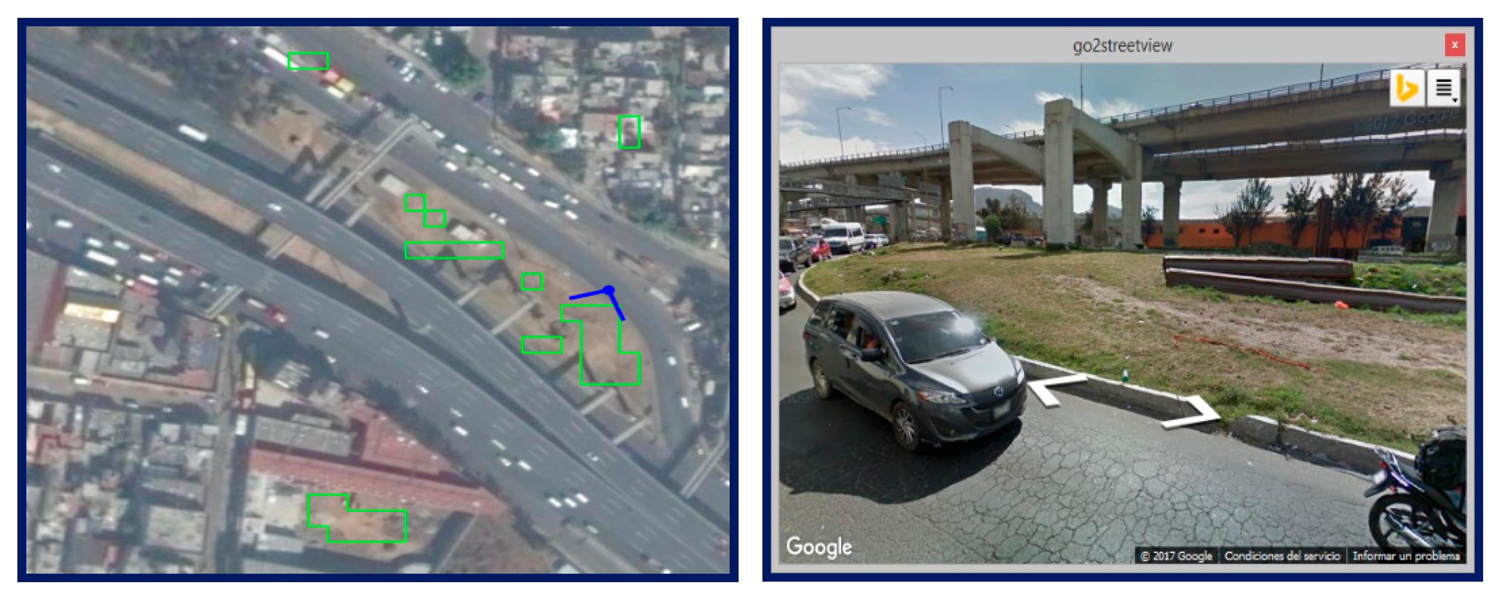
2.3. Identification of Potential Planting Sites

For this study, generally any site without buildings or paving that was also reported as having urban land use within the 16 boroughs that make up Mexico City was considered as a potential planting site [27]. The Milpa Alta borough was not considered because urban land use was not reported. The information was processed in ArcGIS version 10.3 ^® [33]. The visualization and coupling with higher spatial resolution Google Earth^® images were carried out in QGIS [34].

The detection and quantification of potentially useful planting spaces were carried out using supervised classification and masking procedures [17,19,20]. Due to the enormous heterogeneity that characterizes Mexico City, each borough’s territory was analyzed individually in order to reduce the number of contrasting elements that could add confusion to the classification. Through field trips, visual analysis of the satellite images and the coupling of the panchromatic image with higher spatial resolution Google Earth^® images [35], we determined the points that served as sites for training and validated the precision of the classification process (Figure 2).

Four cover classes were defined for all boroughs: trees, grass, bare soil and impervious surface. For the first three classes, training sites and sites to assess the precision of the classification were identified (

Table 2. Training and validation sites by type of cover.

Cover	Number of Training Sites	Number of Validation Sites	Training Area by Type of Cover (ha)
Tree	140	40	0.504
Grass	100	40	0.360
Bare soil	80	40	0.288
Impervious surface	0	40	0

). In order to analyze each borough’s territory in terms of total green area (trees, grass and bare soil) vs. impervious surface (houses, buildings, streets, avenues, etc.), the impervious surface class was added with the inclusion of any surface not covered by trees, grass or bare soil. For validation purposes, 40 points were taken for each defined cover class per borough.

Before executing the supervised classification algorithm, an analysis of the separability of the classes was carried out by performing an unsupervised classification with the iterative self-organizing data analysis technique (ISODATA) algorithm due to the spectral proximity of bare soil to some impervious surfaces such as roofs. With the established training sites, the spectral signature for each type of cover was obtained, and the supervised classification was performed with each spectral signature using the Maxlike (maximum likelihood) algorithm individually in order to obtain thematic maps of the covers required for each borough [36,37].

Masking techniques [22] and map algebra were used to remove the confusion between the “impervious” and “bare soil” classes. Classification accuracy assessment sought to demonstrate that within the impervious class, the buildings are the elements in conflict with the bare soil, so their height was used to differentiate them. The DTM was subtracted from the DSM, which resulted in a new DEM with the heights of the objects in relation to the ground [22], negative values for areas with depressions, zero values for ground level, and values greater than zero for any element with height greater than zero meters. Subsequently, this DEM was resampled to the same pixel size of the satellite image to finally be reclassified and obtain a thematic map with height categories. From this, it was decided that pixels with values from negative to positive with a maximum value of 0.9 m should be considered as ground in order to avoid the exclusion of sites such as planters and roundabouts. This recategorized map served as a mask to correct confusion errors in the bare soil class.

Subsequently, the thematic maps of sites covered with grass and those with bare soil were vectorized, excluding sports fields, which mostly have bare soil or are covered with grass. Sports areas were identified in the c3 vector information layer. Finally, the areas within each borough were quantified to obtain the total hectares representing the detected potential spaces (Figure 3).

2.4. Classification Accuracy Assessment

When classifying the covers individually, there was a possibility of pixels being assigned to more than one class, so the existing confusions were verified through map algebra, specifically with the following interactions: (trees × grass), (trees × soil) and (grass × soil). Analyzing the different pixels with the help of the panchromatic image and Google Earth^® images [38] allowed them to be reassigned to the class to which they belonged. Subsequently, the 0.29% of pixels previously selected as reference data (2330; of which 610, 580, 540 and 600 belong to the tree, grass, bare soil and impervious classes, respectively), were analyzed in a confusion matrix by taking them as field truth vs. the assigned class [39]. The Kappa index and overall accuracy were used to evaluate the degree of precision of the performed classifications [40].

3. Results

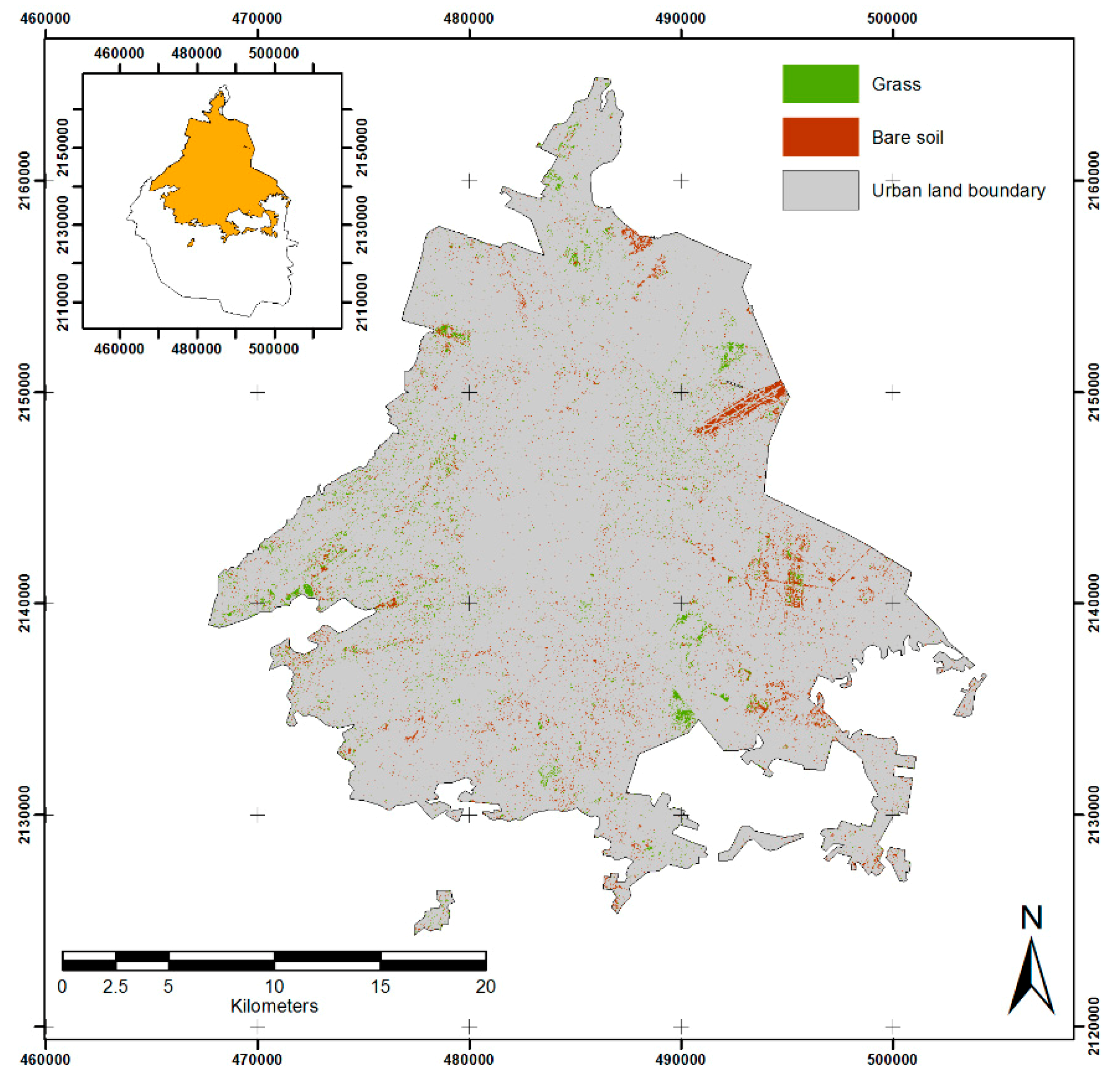
3.1. Location and Quantification of Potential Planting Sites

In all boroughs, sites covered with grass or bare soil were detected (see columns B and C in

Table 3. Potential planting area and total green area in Mexico City’s boroughs.

Borough	Tree (A) ha	Grass (B) ha	Bare Soil (C) (ha)	Potential Sites (B + C) (ha)	Sports Areas (D) (ha)	Total (A + B + C + D) (ha) (%)
Álvaro Obregón	944.8	235.7	196.3	432.1	15.4	1392.4 (13.8)
Azcapotzalco	291.2	24.2	62.1	86.3	15.5	393.0 (3.9)
Benito Juárez	218.3	3.2	9.4	12.7	1.6	232.5 (2.3)
Coyoacán	889.7	51.0	154.1	205.1	35.2	1130.0 (11.2)
Cuajimalpa	169.1	103.3	34.3	137.6	0.3	307.1 (3.1)
Cuauhtémoc	300.2	19.5	41.8	61.3	1.8	363.4 (3.6)
Gustavo A. Madero	673.5	167.4	150.2	317.6	55.6	1046.7 (10.4)
Iztacalco	141.6	34.8	48.2	83.0	14.4	239.0 (2.4)
Iztapalapa	515.5	159.5	410.2	569.6	69.1	1154.2 (11.5)
La Magdalena Contreras	212.9	24.3	23.2	47.4	1.0	261.4 (2.6)
Miguel Hidalgo	972.7	160.1	140.2	300.3	5.6	1278.6 (12.7)
Tláhuac	71.2	17.2	108.4	125.6	7.8	204.6 (2.0)
Tlalpan	864.6	56.9	147.3	204.2	11.2	1080.0 (10.7)
Venustiano Carranza	202.2	97.7	256.0	353.8	15.8	571.8 (7.7)
Xochimilco	232.6	95.9	68.1	164.0	6.0	402.6 (4.0)
Total	6700.3	1250.7	1850	3100.7	256.4	10,057.4 (100.0)

) and considered potentially useful for increasing the currently wooded area (Figure 4). These sites vary in size, with the smallest being an area of approximately 36 m² (pixel size); most of them are located in median strips, parks and roundabouts. The borough of Iztapalapa has the most extensive available area of potential planting sites, while the borough of Benito Juárez has the smallest available area, with 569.6 ha and 12.7 ha, respectively (Table 3).

3.2. Existing Tree Canopy Cover

The tree canopy cover of the 15 boroughs reporting urban land use in their demarcation was quantified, finding an average of 10.6%. The Miguel Hidalgo borough has the largest wooded area with 21% cover, while Tláhuac has the lowest cover with just 3.2% of its area (

Table 4. Estimated canopy cover in 15 Mexico City boroughs.

Borough	Urban Land (ha)	Tree (ha)	Canopy Cover (%)
Álvaro Obregón	6207	944.8	15.2
Azcapotzalco	3350	291.2	8.7
Benito Juárez	2668	218.3	8.1
Coyoacán	5388	889.7	16.5
Cuajimalpa	1717	169.1	9.8
Cuauhtémoc	3250	300.2	9.2
Gustavo A. Madero	7833	673.5	8.6
Iztacalco	2308	141.6	6.1
Iztapalapa	10,740	515.5	4.8
La Magdalena Contreras	1519	212.9	14.0
Miguel Hidalgo	4636	972.7	21.0
Tláhuac	2252	71.2	3.2
Tlalpan	5081	864.6	17.0
Venustiano Carranza	3383	202.2	6.0
Xochimilco	2723	232.6	8.5
Total	63,055	6700.3
Mean			10.6

).

3.3. Total Green Area Surface vs. Impervious Surface

Figure 5 displays a useful measure to estimate the degree of “greenness” of the boroughs, in which areas with cover (or permeable cover) of vegetation are compared with impervious areas (grey surface) such as streets and buildings. The Miguel Hidalgo borough has the highest percentage of surface covered by green area, while the Benito Juárez borough has the lowest percentage, with 27.6% and 8.7%, respectively. In regard to the impervious area, the same ratio is kept, but in the opposite direction; Benito Juárez has 91.3% of this type of cover, while Miguel Hidalgo has an estimated 72.4% (

Table 5. Green area surface vs. impervious surface (grey surface) in Mexico City’s boroughs.

Borough	Total Green Area Surface (%)	Impervious Surface (%)
Álvaro Obregón	22.4	77.6
Azcapotzalco	11.7	88.3
Benito Juárez	8.7	91.3
Coyoacán	21.0	79.0
Cuajimalpa	17.9	82.1
Cuauhtémoc	11.2	88.8
Gustavo A. Madero	13.4	86.6
Iztacalco	10.4	89.6
Iztapalapa	10.7	89.3
La Magdalena Contreras	17.2	82.8
Miguel Hidalgo	27.6	72.4
Tláhuac	9.1	90.9
Tlalpan	21.3	78.7
Venustiano Carranza	16.9	83.1
Xochimilco	14.8	85.2

).

3.4. Potential Tree Canopy Cover, Technical and Market Potential

The PTCC results from the sum of values of columns B, C and D in Table 2. The technical potential is calculated by the sum of the values of columns A, B, C and D. Finally, a rough approximation of the market potential would result from the sum of the values of columns B and C only. The portion corresponding to the sports areas that cannot be considered for planting more trees due to their land use was subtracted from the initial result (

Table 6. Percentages of canopy cover in Mexico City.

Borough	Tree Canopy Cover (%)	Potential Tree Canopy Cover (%)	Technical Potential (%)	Market Potential (%)
Álvaro Obregón	15.2	7.2	22.4	7.0
Azcapotzalco	8.7	3.0	11.7	2.6
Benito Juárez	8.2	0.5	8.7	0.48
Coyoacán	16.5	4.5	21.0	3.8
Cuajimalpa	9.8	8.0	17.9	8.0
Cuauhtémoc	9.2	1.9	11.2	1.9
Gustavo A. Madero	8.6	4.8	13.4	4.1
Iztacalco	6.1	4.2	10.4	3.6
Iztapalapa	4.8	5.9	10.7	5.3
La Magdalena Contreras	14.0	3.2	17.2	3.1
Miguel Hidalgo	21.0	6.6	27.6	6.5
Tláhuac	3.2	5.9	9.1	5.6
Tlalpan	17.0	4.2	21.3	4.0
Venustiano Carranza	6.0	10.9	16.9	10.5
Xochimilco	8.5	6.2	14.8	6.0

).

3.5. Classification Accuracy Assessment

The pixels of tree, grass, bare soil, and impervious classes constituted 0.034%, 0.151%, 0.098%, and 0.005%, respectively, of the total classified pixels. The identification of the four covers of interest from the SPOT 6 satellite image was carried out with acceptable accuracy (

Table 7. Confusion matrix for the land cover classification of Mexico City.

Classes	Tree	Grass	Bare Soil	Impervious	Total	User Accuracy (%)	Commission Error (%)
Tree	562	0	0	4	566	99	1
Grass	3	542	3	5	553	98	2
Bare soil	1	1	467	9	478	98	2
Impervious	44	37	70	582	733	79	21
Total	610	580	540	600	2330
Producer accuracy (%)	92	93	86	97
Commission error (%)	8	7	14	3
Overall accuracy (%)	92.4

). The Kappa index value was 0.89855.

4. Discussion

Although there is currently no clearly defined reference parameter for green area per inhabitant or on the ideal TCC, some cities have adopted a management plan for their urban forests with the goal of increasing tree cover. For example, 20% was reported for Baltimore, 23% for New York, 23% for Seattle, 21% for Los Angeles, 31% for Minneapolis, 32.5% for St. Paul and 22% for Woodbury [25,27,29,41,42], so that such an average could serve as a reference. In this sense, Mexico City is below the average with only 10.6% tree canopy cover, with the possibility of reaching 15.5% if the current TCC plus the percentage added by the market potential is considered; even so, the percentage is still lower than that reported by the cities mentioned.

In the city’s land cover maps, it is not only important to locate both current and potential green areas, but also to locate and quantify the impervious surface, because in this way it is possible to detect the sites with the greatest need for wooded areas and locate those that can potentially act as heat islands [35].

Although the present study detected and quantified the total area with potential to be used as planting spaces due to their permeable surface, it is necessary to consider a series of criteria to discriminate the places that, for various reasons, do not fully comply with any of the defined requirements, and thus determine the market potential and identify surface that is actually usable. For example, although the canopy of certain trees is particularly good for producing a large shaded area, it can also retain heat under it during the night. As such, a canopy cover should not form a continuum in order to allow adequate ventilation and thus allow trapped radiation to escape during the night [9,43]. On the other hand, previous research even discards sites where the potential cover of adult trees overlaps with that of existing trees, or where there is a potential conflict with any other type of existing infrastructure [26,27].

In this sense, the first approximation to determine the market potential in this research was made by establishing detected sites that overlapped with sports areas as exclusion criteria [31], as such sites already have a defined land use which makes them incompatible with the establishment of more trees [25,44]. In addition, ascertaining which of the detected spaces are public and which are private, and identifying under which level of government or under which institutions the safekeeping of such spaces is entrusted are also of interest for the purposes of this research.

Therefore, the first steps are to locate and quantify the potential areas; to determine the market potential; to set a specific goal to be achieved (or that needs to be resolved) in regards to the place where an increase in tree cover is intended. For example, the main objective of the establishment of green areas in the city of Port Phillip, Melbourne, Australia, is the mitigation of the heat island effect [35], while in Minneapolis, Minnesota, USA, strategic tree planting was implemented in order to save electricity following the acquirement of a land map of the city [28]. Even decreasing the pressure for recreational use of existing green areas can be a very important objective to consider [45].

When recognizing sites with planting potential and setting specific objectives for the establishment of new tree areas, it should be remembered that the final selection of species under such specifications will depend on a multiplicity of conditions such as local climate, soil, water availability, and community norms and preferences [46,47] in order to avoid the current problems prevailing in the vast majority of the trees that make up the urban forest as a whole [48,49].

For the final and real estimation of potential planting spaces (market potential), even the opinions of neighbors and others close to the green area in question must be considered; for example, a recurrent unfavorable point of planting in urban parks is that such areas generate a perception of insecurity compared to areas covered with mowed grass [50]; however, this situation can be reversed if the spatial configuration of the area and the structure of the trees are taken into account [51]. Under this scenario, it is possible to recover abandoned spaces and turn them into pleasant places for the generation of environmental services.

5. Conclusions

The classification of covers, namely tree canopies, impervious surface, grass and bare soil, had an accepted average accuracy (kappa of 0.89). While the detected sites covered with grass and bare soil were considered potentially useful areas to plant more trees and subsequently increase the wooded area of Mexico City’s urban area, these sites must be filtered or discriminated by a series of criteria such as land use in order to retain those that are free of any restrictions. The SPOT 6 satellite images and the use of GIS proved to be economical, efficient and relatively precise inputs for the detection and quantification of the covers examined in this study. However, it is necessary to consider the use of higher spatial resolution satellite images given the conditions of Mexico City. When comparing the results with those from 2010, it was possible to make a quantitative assessment of the urban forest dynamics in Mexico City’s area, in which a decrease of 14% was found. Finally, the results of this work can be used to assist in the planning of programs for the recovery and planting of sites devoid of tree cover in Mexico City’s urban area.

References

1. Simpson, J.R.; McPherson, E.G. Simulation of tree shade impacts on residential energy use for space conditioning in Sacramento. Atmos. Environ. 1997, 32, 69–74. [Google Scholar] [CrossRef]
2. Xiao, Q.; McPherson, E.G. Rainfall interception by Santa Monica’s municipal urban forest. Urban Ecosyst. 2003, 6, 291–302. [Google Scholar] [CrossRef]
3. Chiesura, A. The role of urban parks for the sustainable city. Landsc. Urban Plan. 2004, 68, 129–138. [Google Scholar] [CrossRef]
4. Harris, W.R.; Clark, R.J.; Matheny, P.N. Arboriculture: Integrated Management of Landscape Trees, Shrubs, and Vines, 4th ed.; Prentice Hall: Upper Saddle River, NJ, USA, 2004. [Google Scholar]
5. Hardin, P.J.; Jensen, R.R. The effect of urban leaf area on summertime urban surface kinetic temperatures. A Terre Haute case study. Urban For. Urban Green. 2007, 6, 63–72. [Google Scholar] [CrossRef]
6. Escobedo, F.J.; Kroeger, T.; Wagner, J.E. Urban forests and pollution mitigation: Analyzing ecosystem services and disservices. Environ. Pollut. 2011, 159, 2078–2087. [Google Scholar] [CrossRef]
7. Ulrich, R.S. Human responses to vegetation and landscapes. Landsc. Urban Plan. 1996, 13, 29–44. [Google Scholar] [CrossRef]
8. Rosenfeld, A.H.; Akbari, H.; Romm, J.J.; Pomerantz, M. Cool communities: Strategies for heat island mitigation and smog reduction. Energy Build. 1998, 28, 51–62. [Google Scholar] [CrossRef]
9. Spronken-Smith, R.; Oke, T. Scale modelling of nocturnal cooling in urban parks. Bound.-Lay. Meteorol. 1999, 93, 287–312. [Google Scholar] [CrossRef]
10. McPherson, E.G.; Simpson, J.R. Potential energy savings in buildings by an urban tree planting programme in California. Urban For. Urban Green. 2003, 2, 73–86. [Google Scholar] [CrossRef]
11. Rosenzweig, C.; Solecki, W.; Parshall, L.; Gaffin, S.; Lynn, B.; Goldberg, R.; Cox, J.; Hodges, S. Mitigating New York City’s heat island with urban forestry, living roofs, and light surfaces. Presented at the 86th American Meteorological Society Annual Meeting, Atlanta, GA, USA, 30 January–2 February 2006. [Google Scholar]
12. Kenney, W.A.; Wassenaer, P.; Satel, A.L. Criteria and indicators ofr strategic urban forest planning and management. Arboric. Urban For. 2011, 37, 108–117. Available online: http://fufc.org/soap/kenney_criteria_and_indicators2011.pdf (accessed on 12 January 2017).
13. Mcpherson, E.G.; Nowak, D.; Heisler, G.; Grimmond, S.; Souch, C.; Grant, R.; Rowantree, R. Quantifying urban forest structure, function, and value: The Chicago Urban Forest Climate Project. Urban Ecosyst. 1997, 1, 49–61. [Google Scholar] [CrossRef]
14. Wang, S.C. An analysis of urban tree communities using Landsat Thematic Mapper data. Landsc. Urban Plan. 1988, 15, 11–22. [Google Scholar] [CrossRef]
15. Akbari, H.; Rose, L.S.; Taha, H. Analyzing land cover of an urban environment using high-resolution orthophotos. Landsc. Urban Plan. 2003, 63, 1–14. [Google Scholar] [CrossRef]
16. Lees, B.G.; Ritman, K. Decision-tree and rule-induction approach to integration of remotely sensed and GIS data in mapping vegetation in disturbed or hilly environments. Environ. Manag. 1991, 15, 823–831. [Google Scholar] [CrossRef]
17. Xiao, Q.; Ustin, S.L.; McPherson, E.G. Using AVIRIS data and multiple-masking techniques to map urban forest tree species. Int. J. Remote Sens. 2004, 25, 5637–5654. [Google Scholar]
18. Renaud, M.R.; Aryal, J.; Chong, A.K. Object-Based Classification of Ikonos Imagery for Mapping Large-Scale Vegetation Communities in Urban Areas. Sensors 2007, 7, 2860–2880. [Google Scholar]
19. Pu, R.; Landry, S. A comparative analysis of high spatial resolution IKONOS and WorldView-2 imagery for mapping urban tree species. Remote Sens. Environ. 2012, 124, 516–533. [Google Scholar]
20. Stow, D.; Coulter, L.; Kaiser, J.; Hope, A.; Service, D.; Schutte, K.; Walters, A. Irrigated Vegetation Assessment for Urban Environments. Photogramm. Eng. Remote Sens. 2003, 69, 381–390. [Google Scholar] [CrossRef]
21. Walton, J.T.; Nowak, D.J.; Greenfield, E.J. Assessing urban forest canopy cover using airborne or satellite imagery. Arboric. Urban For. 2008, 34, 334–340. Available online: https://www.ncrs.fsfed.us/pubs/jrnl/2008/nrs_2008_walton_002.pdf (accessed on 24 February 2017).
22. Höfle, B.; Hollaus, M. Urban vegetation detection using high density full-waveform airborne lidar data-combination of object-based image and point cloud analysis. In ISPRS TC VII Symposium—100 Years ISPRS; Wagner, W., Székely, B., Eds.; IAPRS: Vienna, Austria, 2010; Volume XXXVIII. [Google Scholar]
23. Moskal, L.M.; Styers, D.M.; Halabisky, M. Monitoring urban tree cover using object-based image analysis and public domain remotely sensed data. Remote Sens. 2011, 3, 2243–2262. [Google Scholar] [CrossRef] [Green Version]
24. Agarwal, S.; Vailshery, L.S.; Jaganmohan, M.; Nagendra, H. Mapping urban tree species using very high resolution satellite imagery: Comparing Pixel-Based and Object-Based Approaches. ISPRS Int. J. Geoinf. 2013, 2, 220–236. [Google Scholar] [CrossRef]
25. McPherson, E.G.; Simpson, J.R.; Xiao, Q.; Wu, C. Million trees Los Angeles canopy cover and benefit assessment. Landsc. Urban Plan. 2011, 99, 40–50. [Google Scholar] [CrossRef]
26. Wu, C.; Xiao, Q.; McPherson, E.G. A method for locating potential tree-planting sites in urban areas: A case study of Los Angeles, USA. Urban For. Urban Green. 2008, 7, 65–76. [Google Scholar] [CrossRef]
27. Parlin, M. Seattle Washington Urban Tree Canopy Analysis Project Report: Looking Back and Moving Forward; Native Communities Development Corporation: Colorado Springs, CO, USA, 2009. [Google Scholar]
28. Bauer, M.; Kilberg, D.; Martin, M.; Tagar, Z. Digital Classification and Mapping of Urban Tree Cover: City of Minneapolis; University of Minnesota: St. Paul, MN, USA, 2011. [Google Scholar]
29. Kilberg, D.; Martin, M.; Bauer, M. Mapping Urban Tree Cover: Object Oriented Image Analysis of QuickBird and Lidar Data; University of Minnesota: St. Paul, MN, USA, 2012. [Google Scholar]
30. McPherson, E.G.; Sacamano, P.L.; Wensman, S. Modeling Benefits and Costs of Community Tree Plantings; USDA Forest Service—Pacific Southwest Research Station: Davis, CA, USA, 1993.
31. Procuraduría Ambiental y del Ordenamiento Territorial del D.F (PAOT). Presente y Futuro de las Áreas Verdes y Arbolado de la Ciudad de Mexico; [Present and Future of the Green Areas and Trees in Mexico City]; PAOT: CDMX, Mexico, 2010. [Google Scholar]
32. Astrium. SPOT 6 & SPOT 7 Imagery User Guide; Astrium Services: Toulouse, France, 2013. [Google Scholar]
33. Environmental Systems Research Institute Inc. (ESRI). ArcGIS Version 10.3; ESRI: Redlands, CA, USA, 2006. [Google Scholar]
34. QGIS Geographic Information System: Open Source Geospatial Foundation Project. 2015. Available online: http://qgis.osgeo.org (accessed on 14 May 2015).
35. Norton, B.A.; Coutts, A.M.; Livesley, S.J.; Harris, R.J.; Hunter, A.M.; Williams, N.S.G. Planning for cooler cities: A framework to prioritise green infrastructure to mitigate high temperatures in urban landscapes. Landsc. Urban Plan. 2015, 134, 127–138. [Google Scholar] [CrossRef]
36. Chuvieco, S.E. Teledetección Ambiental: La Observación de la Tierra Desde el Espacio; [Environmental Tele Detection: The Earth Observation from Space]; Ariel: Barcelona, Spain, 2002. [Google Scholar]
37. Tso, B.; Mather, P.M. Classification Methods for Remotely Sensed Data, 2nd ed.; Taylor & Francis Group: Boca Raton, FL, USA, 2009. [Google Scholar]
38. Estoque, R.C.; Murayama, Y.; Akiyama, C.M. Pixel-based and object-based classifications using high- and medium- spatial-resolution imageries in the urban and suburban landscapes. Geocarto Int. 2015, 30, 1113–1129. [Google Scholar] [CrossRef] [Green Version]
39. Congalton, R.G. A review of assessing the accuracy of classifications of remotely sensed data. Remote Sens. Environ. 1991, 37, 35–46. [Google Scholar] [CrossRef]
40. Landis, J.R.; Koch, G.G. The measurement of observer agreement for categorical data. Biometrics 1977, 33, 159–174. Available online: http://www.jstor.org./stable/2529310 (accessed on 18 March 2017). [CrossRef] [Green Version]
41. Galvin, M.F.; Grove, J.M.; O’Neal-Dunne, J.P.M. A Report on Baltimore City’s Present and Potential Urban Tree Canopy; Maryland Department of Natural Resources: Annapolis, MD, USA, 2006.
42. Grove, J.M.; Cadenasso, M.L.; Burch, W.L.; Pickett, S.T.A.; Schwarz, K.; O’Neal-Dunne, J.; Wilson, M.; Troy, A.; Boone, C. Data and methods comparing social structure and vegetation structure of urban neighborhoods in Baltimore, Maryland. Soc. Nat. Resour. 2006, 19, 117–136. [Google Scholar] [CrossRef]
43. Dimoudi, A.; Nikolopoulou, M. Vegetation in the urban environment: Microclimatic analysis and benefits. Energy Build. 2003, 35, 69–76. [Google Scholar] [CrossRef] [Green Version]
44. Rowntree, R.A. Forest canopy cover and land use in four Eastern United States cities. Urban Ecol. 1984, 8, 55–67. [Google Scholar] [CrossRef]
45. Van Elegem, B.; Embo, T.; Muys, B.; Lust, N. A methodology to select the best locations for new urban forests using multicriteria analysis. Forestry 2002, 75, 13–23. [Google Scholar] [CrossRef]
46. Bowler, D.E.; Buyung-Ali, L.; Knight, T.M.; Pullin, A.S. Urban greening to cool towns and cities: A systematic review of the empirical evidence. Landsc. Urban Plan. 2010, 97, 147–155. [Google Scholar] [CrossRef]
47. Pataki, D.E.; Carreiro, M.M.; Cherrier, J.; Grulke, N.E.; Jennings, V.; Pincetl, S.; Pouyat, R.V.; Whitlow, T.H.; Zipperer, W.C. Coupling biogeochemical cycles in urban environments: Ecosystem services, green solutions, and misconceptions. Front. Ecol. Environ. 2011, 9, 27–36. [Google Scholar] [CrossRef]
48. Chacalo, A.; Aldama, A.; Grabinsky, J. Street tree inventory in Mexico City. J. Arboric. 1994, 20, 222–226. Available online: http://joa.isa-arbor.com/request.asp?JournalID=1&ArticleID=2632&Type=2 (accessed on 13 December 2016).
49. Procuraduría Ambiental y del Ordenamiento Territorial (PAOT). Manejo y Conservación de Áreas Verdes: Informe Annual; [Management and Conservation of Green Areas. Annual Report]; PAOT: CDMX, Mexico, 2003; Available online: http://paot.org.mx/centro/paot/informe2003/temas/manejo.pdf (accessed on 30 April 2017).
50. Parsons, R. Conflict between ecological sustainability and environmental aesthetics: Conundrum, canard or curiosity. Landsc. Urban Plan. 1995, 32, 227–244. [Google Scholar] [CrossRef]
51. Randall, T.A.; Churchill, C.J.; Baetz, B.W. A GIS-based decision support system for neighbourhood greening. Environ. Plan. B Plan. Des. 2003, 30, 541–563. [Google Scholar] [CrossRef]
Figure 1. Study area delimited by Mexico City’s urban land.
Forests 11 00423 g001
Figure 2. Training sites for bare soil (green squares on the left) located at I. Zaragoza Avenue in the Iztapalapa borough of Mexico City.
Forests 11 00423 g002
Figure 3. Flowchart for the identification of potential planting sites.
Forests 11 00423 g003
Figure 4. Potential planting sites (bare soil) in Mexico City’s urban land.
Forests 11 00423 g004
Figure 5. Green area vs. impervious surface in Mexico City.
Forests 11 00423 g005