Article

Uncertainty in Forest Net Present Value Estimations

1
Department of Forest Sciences, University of Helsinki, Latokartanonkaari 7, 00014 Finland
2
Simosol Oy, Asema-aukio 2, 11130 Riihimäki, Finland
3
MTT, Economic Research, Latokartanonkaari 9, 00790 Helsinki, Finland
*
Author to whom correspondence should be addressed.
Forests 2010, 1(3), 177-193; https://doi.org/10.3390/f1030177
Submission received: 9 August 2010 / Revised: 31 August 2010 / Accepted: 10 September 2010 / Published: 27 September 2010
(This article belongs to the Special Issue Feature Papers)

Abstract

:
Uncertainty related to inventory data, growth models and timber price fluctuation was investigated in the assessment of forest property net present value (NPV). The degree of uncertainty associated with inventory data was obtained from previous area-based airborne laser scanning (ALS) inventory studies. The study was performed, applying the Monte Carlo simulation, using stand-level growth and yield projection models and three alternative rates of interest (3, 4 and 5%). Timber price fluctuation was portrayed with geometric mean-reverting (GMR) price models. The analysis was conducted for four alternative forest properties having varying compartment structures: (A) a property having an even development class distribution, (B) sapling stands, (C) young thinning stands, and (D) mature stands. Simulations resulted in predicted yield value (predicted NPV) distributions at both stand and property levels. Our results showed that ALS inventory errors were the most prominent source of uncertainty, leading to a 5.1–7.5% relative deviation of property-level NPV when an interest rate of 3% was applied. Interestingly, ALS inventory led to significant biases at the property level, ranging from 8.9% to 14.1% (3% interest rate). ALS inventory-based bias was the most significant in mature stand properties. Errors related to the growth predictions led to a relative standard deviation in NPV, varying from 1.5% to 4.1%. Growth model-related uncertainty was most significant in sapling stand properties. Timber price fluctuation caused the relative standard deviations ranged from 3.4% to 6.4% (3% interest rate). The combined relative variation caused by inventory errors, growth model errors and timber price fluctuation varied, depending on the property type and applied rates of interest, from 6.4% to 12.6%. By applying the methodology described here, one may take into account the effects of various uncertainty factors in the prediction of forest yield value and to supply the output results with levels of confidence.

1. Introduction

Estimates of the economical value of forest property are needed for many purposes, e.g., in the real estate business, land divisions and exchanges and for considering forestry investment. In addition, the International Financial Reporting Standards (IFRS) require that forest enterprises present systematically computed estimates of the value of their forested land annually.
One method for deriving the economic value of a forest stand or property is to calculate the difference between the present values (net present value, NPV) of all future expected revenues and expenses. This approach is referred to as the forestry yield value method [1] and it is based on the fundamental ideas of forest economics [2]. The estimation of future chains of forest stand management and the flow of revenues and expenses are most commonly performed on the basis of the harvest and silviculture recommendations presented in the respective forest management plan. Revenues and expenses are estimated, based on the wood production predictions that are commonly determined by simulation and optimization computations carried out by specific forest-planning software systems. Decisive issues regarding the determination of forestry yield value include determination of the optimal rotation length, the timing and intensity of harvests, timber stumpage prices, silvicultural costs and the applied interest rate. The NPV of forested land is subject to various uncertainties. The sources of uncertainty include growth and yield models used in the simulators, development of timber prices, the rate of interest used and uncertainties in the input data.
Acquisition of forest-planning data is currently in a phase of radical change. In Finland, operative forest planning is evolving into a methodology by which stock characteristics are estimated by means of tree-wise measured sample plots and area-based statistical features of airborne laser scanning (ALS) data and digital aerial photographs. Estimation of forest characteristics will be performed, using the nonparametric k-nearest neighbor (k-NN) or k-most similar neighbor (k-MSN) method [3]. With respect to the estimation of stand mean characteristics (e.g., [4,5,6,7]) and tree species- or timber assortment-specific characteristics [8,9,10,11], it has become possible to achieve at least the same level of accuracy using low-pulse ALS data as that found in traditional standwise forest inventory (SWFI). Overviews on the use of ALS in forest inventory can be found in [12,13,14,15].
Currently, a crucial question that remains is how to integrate this new inventory data into forest-planning computations. It is then essential to be aware of how inventory data obtained at various accuracies affect the simulation end results, which have a significant influence on the forest owner’s economic return. Thus, a starting point for the study was the state of change currently present in operative forest planning, in which traditional compartment inventories are being replaced by ALS-based inventories.
Reliable inventory data are essential for forestry yield value simulations. In assessing the state of a stand, the estimates may differ significantly from the real situation, due to the inventory method used. This aspect can be studied using cost-plus-loss analyses, in which the expected losses due to suboptimal decisions are added to the total forest inventory costs ([16,17]). The cost-plus-loss approach was widely utilized in recent forest inventory- and planning-related research (e.g., [18,19,20,21,22,23,24]).
The growth of trees or timber stock is a highly significant factor affecting forestry yield value. From the standpoint of forest property valuation, the rate of growth is a decisive factor with respect to rotation length and therefore influences yield value computations to a great extent. Since tree growth is difficult to measure directly, it must be estimated by models based on other measurable tree characteristics. Growth models can be divided into tree- and stand-level models (e.g., [25]).
Forest growth simulators are applied for updating measured forest resource data and for predicting future growth to assess silvicultural measures and time of harvests. Growth simulators incorporate numerous models for predicting various forest characteristics and their development. These models can never completely portray the underlying phenomena and their output estimates therefore include a degree of uncertainty. The degree of uncertainty is dependent on the functioning of individual models and the interaction between them. Models applied for simulating forest growth form a complex entity that often complicates the analysis of individual model uncertainty ([25,26]).
Uncertainty related to forest growth modeling has been studied, e.g., by Gertner and Dzialowy [27], Mowrer [28] and Kangas ([26,29]). These studies have mainly focused on the influence of various uncertainty components in growth model functioning. However, Mäkinen et al. [25] and Mäkinen [30] showed that instead of analyzing individual models, the model chains implemented by the simulators should be scrutinized as a whole.
The development of timber assortment prices is one of the most significant factors in forest property valuation computations. A major part of a stand’s yield value is generated at the final harvest, in which case the timing of the final harvest and the prices of the most valuable timber assortments (saw-wood and intermediate logs) at that time are especially important. Saw-wood log outturn is, in turn, influenced by the (company-specific) bucking rules and quality criteria in effect at that time. Timber prices at the stand level are further influenced by harvest conditions, size of the logging site and near-hauling distance.
When estimating the value of a forest property, the most common way to incorporate timber prices is to apply mean prices based on the realized prices of the past [31]. The basic assumption then is that future price development is in accordance with past development. A more advanced, and also complicated, approach is to try to predict future timber price development based on realized past price development, by which long-term trends can be depicted and factors causing price peaks identified. Such predictions can be carried out e.g., by using geometric mean-reverting (GMR, [32,33,34]) or geometric Brownian motion (GBM, [35,36,37]) price processes.
This study builds on a paper by Holopainen et al. [38]. They studied uncertainties related to compartment level field inventories, area-based ALS-inventories, growth models and timber price fluctuations when computing net present value over the rotation length on the stand level. According to their results, growth models applied in forest planning simulation computations proved to be the most significant source of uncertainty in stand level computations. However, a property (or estate) is the unit in operational forest value estimations produced for the purposes of e.g., real estate business, land exchanges and land divisions. The effects of various sources of uncertainty on the value of forest property cannot be obtained simply by aggregating the uncertainties observed at stand level, because the deviations from average or true value estimates between various stands tend to partly cancel out each other [38]. Thus, additional model simulations are needed to obtain the overall level of uncertainty for typical sized forest estates.

2. Objective

The objective of the study was to analyze the effect of uncertainty factors related to inventory data, growth models and timber price fluctuation on the prediction of forest property-level NPV. The term uncertainty here refers to the variation in estimated forest NPVs caused by errors in inventory data, random errors in growth and yield projections and random variations in timber assortment prices. The degree of uncertainty-related inventory data was derived from previous studies dealing with area-based ALS inventories at the stand level. The effects of timber price fluctuation were depicted with stochastic GMR price models. Forest property-level NPVs were estimated using three alternative rates of interest (3%, 4% and 5%). The study was carried out applying the Monte Carlo (MC) simulation method and using stand-level growth and yield projection models.

3. Material and Methods
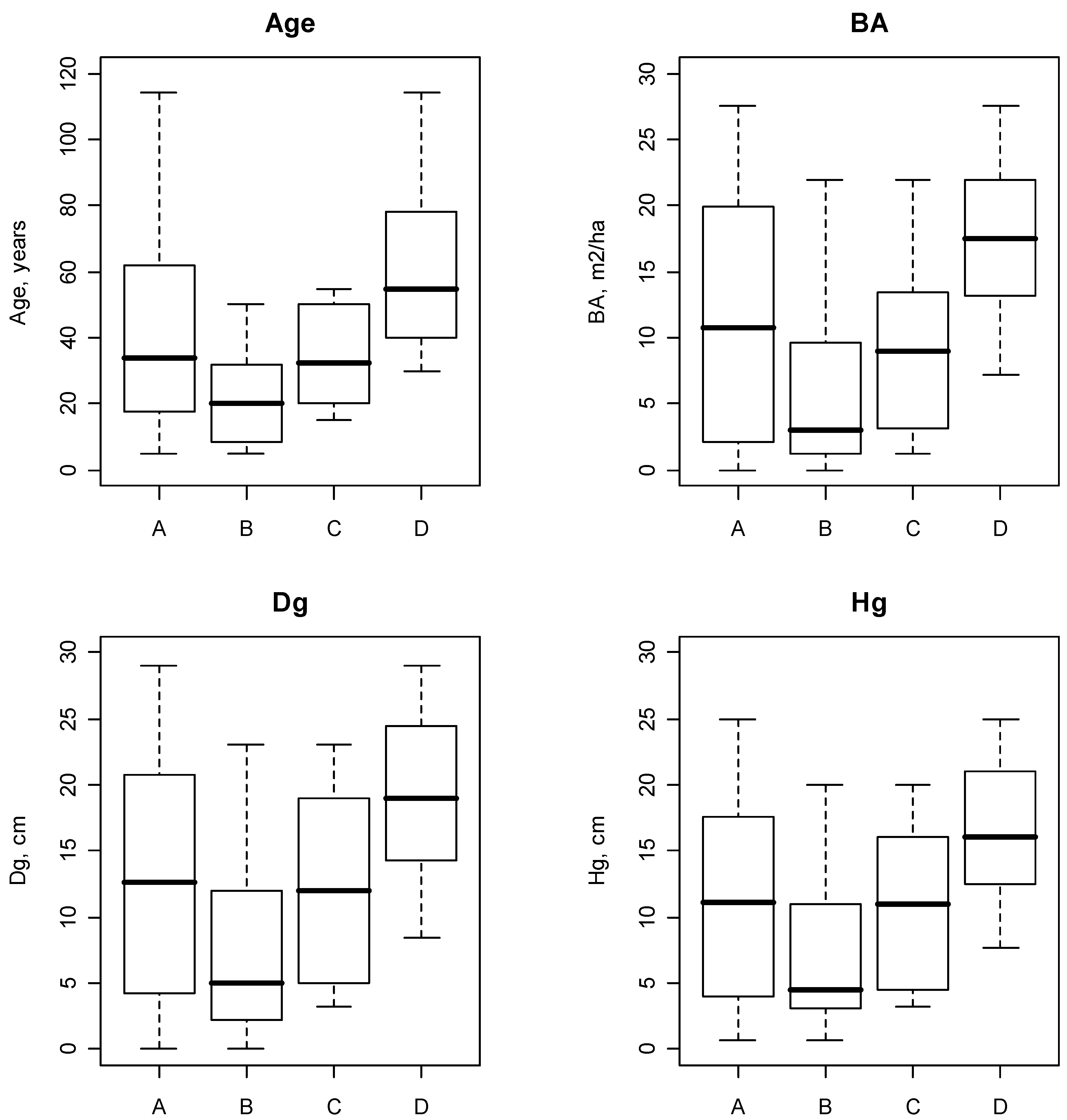
3.1. Data

The starting point of the investigation consisted of four simulated forest properties having varying compartment structures: a property having an even development class distribution (A), sapling stands (B), young thinning stands (C) and mature stands (D). Variation in basic stand characteristics in properties can be seen in Figure 1. All properties included some variation between stand development classes. In forest property A, where development class distribution was even, age, basal area, mean diameter and mean height varied from 5 to 144 years, 0 to 27.5 m2/ha, 0 to 29.0 cm and 0.6 to 26.0 m, respectively. In sapling-dominated forest property B, the respective variations were 5–50 years, 0–22.0 m2/ha, 0–23.0 cm and 0.6–20.0 m. Young thinning stands predominated in forest property C and the variations were 15–55 years, 1.3–22.0 m2/ha, 3.2–23.0 cm and 3.2–20.0 m as in forest property D, which was dominated by mature stands with respective variations of 30–114 years, 7.2–27.5 m2/ha, 8.4–29.0 cm and 7.7–25.0 m. We assumed that these stand characteristics were estimated with area-based ALS inventory.
Figure 1. Variation in stand characteristics within the forest properties: A (having an even development class distribution), B (sapling stands), C (young thinning stands) and D (mature stands). Top left: age; top right: basal area (BA); bottom left: mean diameter (Dg); and bottom right: mean height (Hg).
Forests 01 00177 g001

3.2. Simulation of the Sources of Uncertainty

The relative importance of the three sources of uncertainty in forest NPV computations was determined by simulating each stand within each forest property repeatedly with the MC method (e.g., [25,26,29,39]). In MC methodology, confidence estimates are obtained by generating an error term from the model's error distribution for each output estimate. The model is run dozens or hundreds of times, the results of which are used to determine the final predicted value error statistics.
The uncertainty caused by random variation in future timber assortment prices is referred to as UPRICE, the uncertainty caused by input data errors UINV and the uncertainty caused by random errors in growth projections is referred to as UGROWTH. The sources of uncertainty were included in the simulations separately and all three simultaneously, enabling us to determine how the different sources of uncertainty affect the NPV distributions. In addition, we simulated each combination with interest rates of 3%, 4% and 5%. The calculations were carried out using SIMO simulation and optimization software (SIMO simulation framework, [40,41]).
UINV, UGROWTH and UPRICE were simulated in a manner similar to that in [38]. The effect of random variation, i.e., measurement and sampling errors, in forest inventory data was taken into account by generating true values from the estimates in the simulation input dataset, using so-called true value models. In this context the term true values refer to simulated (not actual) true stand attribute values. The true value models were constructed so that trends, distribution shapes and correlations between the various attributes were taken into account.
Data for modeling true values of ALS inventory were based on a study area in northeastern Finland that included 89 stands. The values for the attributes were estimated and measured at the tree species stratum level and the estimates were based on the k-MSN procedure (for details see [42]. The dataset used is described in further detail in Mäkinen et al. [43]. The uncertainty caused by the stand-level growth models was taken into account by including a random variation component in the growth projections. A more detailed description of random component in the growth predictions can be found in [38]. However, the autocorrelation component included in [38] was excluded from these simulations.
Timber prices were modeled using a GMR process that utilized historical price statistics on real stumpage prices in Finland between January 1986 and August 2008. The price statistics were given separately for saw logs and pulpwood for the three main commercial timber species in Finland: Scots pine (Pinus sylvestris L.), Norway spruce (Picea abies (L.) H. Karst.) and birch (Betula L.) [38].
The development of each stand was simulated until the next regeneration harvest, or a maximum of 100 years, using a one-year timestep, and repeating the entire simulation process 100 times for each source of uncertainty and interest rate combination.
The thinning schedules were based on silvicultural recommendations of the forestry extension organization Tapio in Finland [44]. The regeneration harvests were done as soon as the 5-year moving average of value growth percentage, or so-called v-value, of the stand was less than the interest rate chosen. To estimate the timber assortment volumes and incomes from the harvests, tree diameter distributions were constructed for each stand before the harvests, using the distribution models by [45,46,47]. The value of each diameter class was then predicted with the taper curve functions of [48] and optimal stem bucking algorithm of [49]. Decisions about when to harvest and regenerate were made at single stand-level and, in this case, without any property-level constraints. This is, of course, a simplification as in some cases the harvest and regeneration decisions are not totally independent. However, we believe that this kind of simplification can be justified as the decision maker aims at simply maximizing the NPV of the forest property.
When summing stand level data to property level correlations were accounted for by generating 100 alternative random timber price scenarios (one for each MC iteration) and thus stands that were generated during the same time step and iteration had similar timber prices. This should guarantee that the variation at the property-level was appropriate.

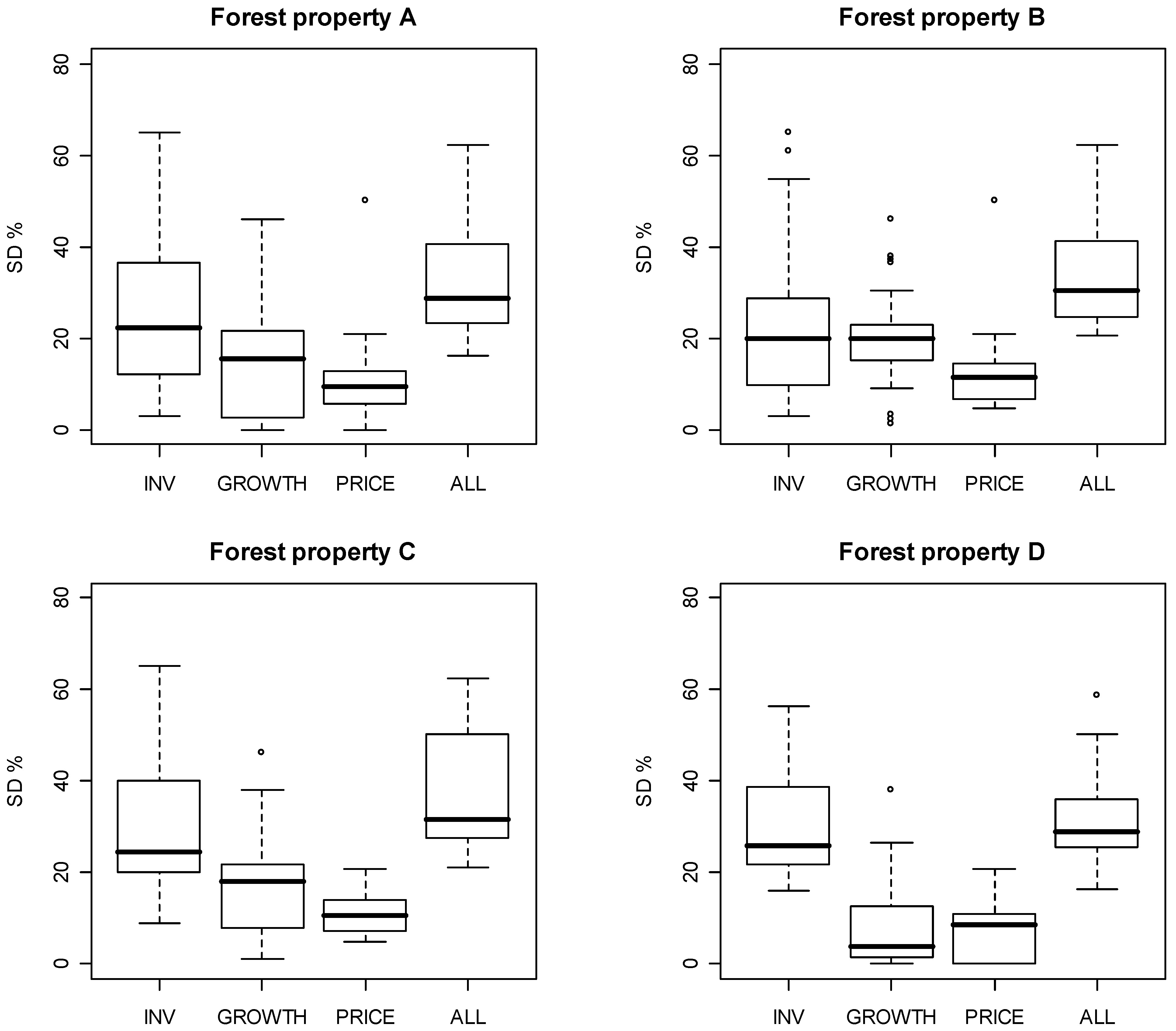
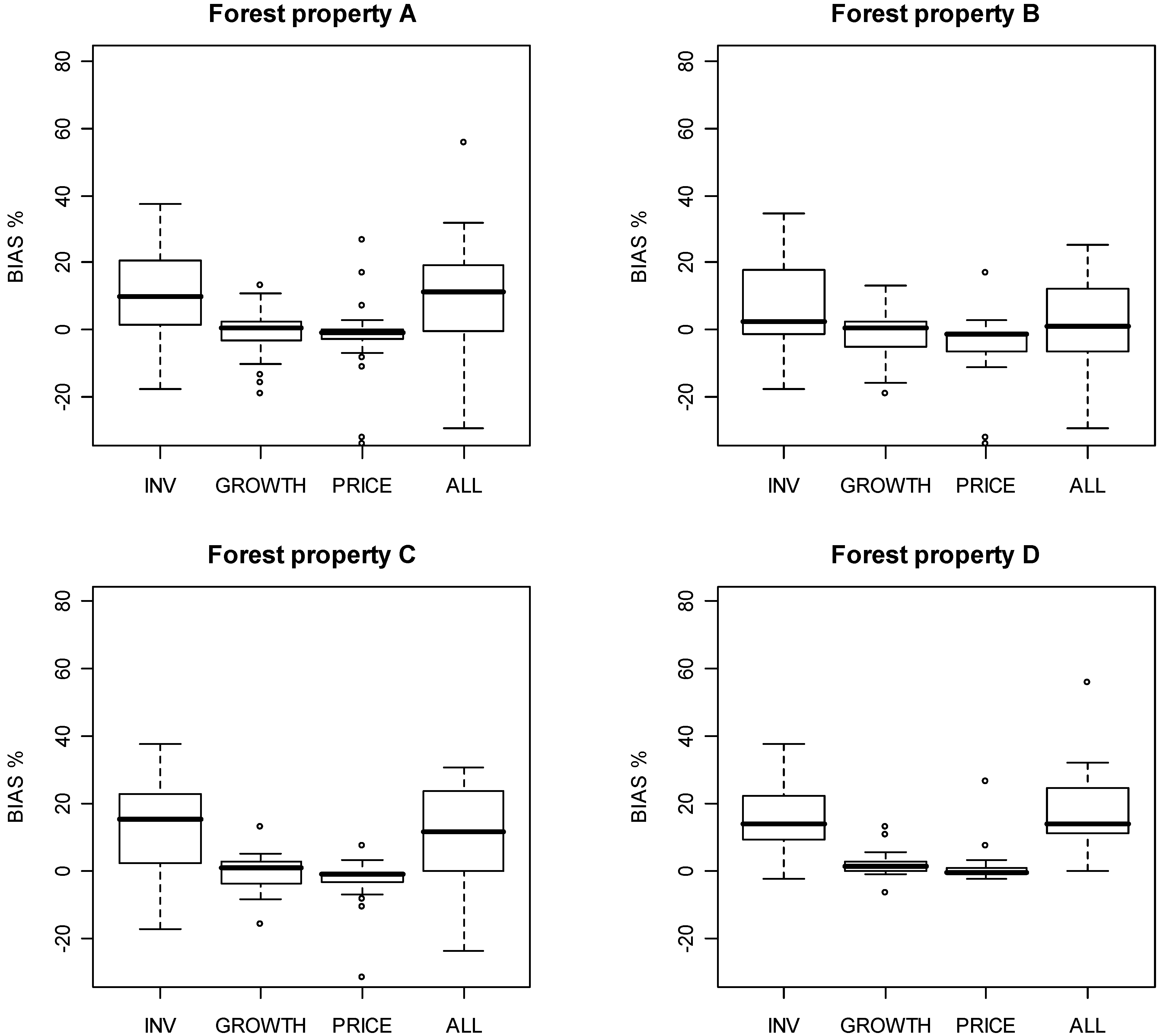
3.3. Analysis of the Uncertainty

The uncertainty in the NPV simulation was analyzed by determining the distributions of the NPVs and comparing them with the reference NPVs simulated from true values, separately for each source of uncertainty and interest rate combination. The simulation computations resulted in predicted yield value (predicted NPV) distributions at the property level.
For each property i, the mean and sd of the NPV distribution, meaniNPV and sdiNPV, respectively, were calculated with Equations (1) and (2).
m e a n i N P V = l = 1 100 ( n p v i l ) × 1 100
s d i N P V = l = 1 100 ( n p v i l m e a n i N P V ) 2 × 1 100
The bias, i.e., the difference between the reference NPVs and means of the NPV distributions of each property i, was calculated as biasiNPV = meaniNPVnpviREF and the relative, or percentual, bias was calculated as bias%iNPV = (meaniNPVnpviREF)/npviREF × 100. We were also interested in the relative variation and thus the relative sd (%) was calculated with Equation (3).
s d % i N P V = l = 1 100 ( ( n p v i l m e a n i N P V m e a n i N P V ) × 100 ) 2 × 1 100

4. Results

The effects of uncertainty related to inventory data, growth models and timber price fluctuation on forest property-level NPVs are summarized in Table 1. The effect of each individual source of error and the combined effect were derived for each forest property type. Computations were carried out using three different rates of interest (3%, 4% and 5%). The effect of the applied rate of interest on the per-hectare NPVs is presented in Table 2. Forest properties A, B, C, and D standwise NPV variation SDs and biases are presented in Figure 2 and Figure 3.
As presented in Table 1, forest inventory-related errors were the most significant source of uncertainty in all of the forest property types analyzed. Inventory-related errors led to a forest property-level relative standard deviation ranging from 5.1% to 7.5% when an interest rate of 3% was applied. The respective biases varied from 8.9% to 14.1%. The effect of inventory-related bias was emphasized, especially in the case of the mature stand property (D).
Table 1. Averages of the relative biases (BIAS%NPV) and standard deviations (SD%NPV) of the simulated NPV distributions of the 25 hectare forest property with given source of uncertainty and interest rate combination.
Active sources of uncertaintyInterest rate
3 % 4 % 5 %
Forest propertyUinventoryUgrowthUpricemeanNPVBIAS%NPVSD%NPVmeanNPVBIAS%NPVSD%NPVmeanNPVBIAS%NPVSD%NPV
A 142,140.912.25.1123,038.614.46.5112,439.918.17.6
A 128,507.91.41.7109,728.82.11.397,236.12.11.4
A 124,846.2−1.53.4106,930.3−0.52.495,661.80.52.0
A143,469.513.26.5125,119.516.46.4115,839.121.76.8
B 87,042.18.97.463,659.016.59.949,849.924.311.1
B 79,864.9−0.14.155,853.22.23.641,231.22.84.4
B 76,160.0−4.75.852,502.4−3.94.739,230.1−2.14.8
B84,661.35.99.362,515.114.49.849,896.324.512.6
C 120,940.713.57.595,619.719.79.480,878.829.612.0
C 107,330.00.73.281,492.22.03.164,357.03.23.3
C 103,493.5−2.96.478,387.9−1.94.962,126.2−0.44.6
C118,141.010.99.495,007.319.09.780,928.529.710.9
D 204,107.414.15.8186,286.615.47.2177,365.518.68.1
D 183,501.92.61.5165,762.02.71.3153,543.82.71.3
D 179,539.00.43.6162,407.20.62.3151,240.51.21.9
D209,108.816.97.3191,775.918.87.4184,321.223.37.3
The active uncertainty sources in each combination are marked with •.A = a property having an even development class distribution,B = a sapling stand property,C = a young thinning stand property,D = a mature stand property.
Table 2. Averages of the relative biases (BIAS%NPV) and standard deviations (SD%NPV) of the simulated NPV distributions per hectare with given sources of uncertainty and interest rate combination.
Active sources of uncertaintyInterest rate
3 % 4 % 5 %
Forest propertyUinventoryUgrowthUpricemeanNPVBIAS%NPVSD%NPVmeanNPVBIAS%NPVSD%NPVmeanNPVBIAS%NPVSD%NPV
A 5,685.612.225.94,921.514.430.44497.618.133.6
A 5,140.31.415.34,389.22.115.53889.42.118.8
A 4,993.8−1.59.94,277.2−0.59.13826.50.58.7
A5,738.813.232.85,004.816.435.34633.621.739.3
B 3,481.78.922.92,546.416.527.71994.024.329.6
B 3,194.6−0.120.62,234.12.220.51649.22.824.6
B 3,046.4−4.712.62,100.1−3.911.61569.2−2.111.6
B3,386.55.934.82,500.614.438.11995.924.541.8
C 4,837.613.529.73,824.819.735.03235.229.640.8
C 4,293.20.717.73,259.72.016.92574.33.220.2
C 4,139.7−2.911.23,135.5−1.99.82485.0−0.49.3
C4,725.610.937.13,800.319.041.13237.129.746.4
D 8,164.314.130.47,451.515.435.47094.618.640.9
D 7,340.12.68.66,630.52.79.26141.82.711.1
D 7,181.60.47.96,496.30.66.66049.61.26.0
D8,364.416.931.27,671.018.833.77372.823.339.1
The active uncertainty sources in each combination are marked with •. A = a property having an even development class distribution, B = a sapling stand property, C = a young thinning stand property, D = a mature stand property.
Figure 2. Variation in relative SD within stands of forest properties (25 ha, interest rate 3%). INV = Uinv, GROWTH = Ugrowth, PRICE = Uprice, ALL = combined error.
Forests 01 00177 g002
The growth model-related uncertainty caused a 1.5–4.1% variation in the simulated property-level NPV-values when an interest rate of 3% was applied. The respective variation biases ranged from −2.9% to 2.6%. Timber price development led to the same degree of uncertainty as the growth models and the relative NPV standard deviations ranged from 3.4% to 6.4% (3% rate of interest) and the biases from −4.7% to 0.4%. The relative combined standard deviation caused by inventory error, growth model error and timber price fluctuation varied, depending on forest property type, from 6.5% to 9.4% and biases from 5.9% to 16.9% (3% interest rate). Biases at the property level should be noted.
The per-hectare results are presented in Table 2. Uncertainty (NPV deviation) at the per-hectare level is significantly higher than that on the forest property level. Uncertainty due to inventory data error, growth model error, and timber price fluctuation varied from 22.9% to 30.4%, 8.6% to 20.6% and 7.9% to 12.6%, respectively, when an interest rate of 3% was applied. The combined NPV deviation varies, depending on forest property type and the applied rate of interest, from 31.2% to 46.4%.
Figure 3. Variation in relative BIAS within stands of forest properties (25 ha, interest rate 3%). INV = Uinv, GROWTH = Ugrowth, PRICE = Uprice, ALL = combined error.
Forests 01 00177 g003

5. Discussion

The study involved the effects of ALS inventory, growth model errors and timber price fluctuation on forest property-level predicted NPVs. The results showed that the greatest source of uncertainty in each type of property studied was ALS inventory errors. These errors led to significant biases at the forest-property level NPV, which should be examined further. The effects of growth modeling errors and timber price fluctuation caused minor standard deviations and biases compared to inventory data errors.
Growth model-related uncertainty was highest in sapling stands and lowest in mature stands, i.e., the longer the simulation period the greater the uncertainty due to growth model errors. On the other hand, the degree of predicted NPV deviation caused by inventory error and timber price fluctuation did not vary significantly in the property types examined.
Different rates of interest (3–5%) led to minor differences in predicted NPV deviation. However, the rate of interest applied has a pronounced influence on the predicted property value and biases (see Table 1 and Table 2).
The relative combined deviation caused by inventory error, growth model error and timber price fluctuation ranged, depending on property type and applied rate of interest, from 6.4% to 12.6%. In other words, the combined deviation was similar to that caused by inventory error alone. Apparently, the various sources of uncertainty tend to neutralize each other.
Property size did not affect the degree of uncertainty, since stand size was set as proportional to property size in the study because our objective was primarily to analyze the effects of various sources of uncertainty on property-level predicted NPV. To determine the effect of property size, the effects of all other sources of uncertainty should be eliminated; these analyses will be performed in future studies.
Our results are directly comparable with those presented by Holopainen et al. [38]. In their study, the uncertainty caused by inventory error, growth model error and timber price fluctuation was scrutinized in a fashion similar to that shown here, but at the stand level. Holopainen et al. [38] showed that the influence of a single source of uncertainty varied from 8.2% (timber price) to 33.2% (growth models) when an interest rate of 3% was applied. When the various sources of error were combined and an interest rate of 3% was applied, the resulting maximum relative NPV was 47.4%. Comparison of our results with those of Holopainen et al. [38] showed that the forest property level deals with a considerably lesser degree of NPV deviation than does stand level. This can also be noted by comparing the property level and per-hectare results of this study (Table 1 and Table 2). Reason for decreased uncertainties related to forest inventory data and growth modeling errors is that if inventory method and growth models are unbiased, the larger and more homogeneous the inventory unit, the smaller the relative standard error achievable. Several remote-sensing related forest inventory studies have revealed that the relative root-mean squared error (rmse) value describing the accuracy of the inventory method is strongly dependent on the size of inventory unit examined (tree, plot, stand, property) and its degree of internal variation (homogeneity) (e.g., [50]).
The reduced variation in NPV due to price fluctuations, when shifting from stand level to property level, is a consequence of two factors. Firstly, the timing harvests and other silvicultural activities are different between stands in different development stages. Secondly, the timber species in various stands are different. Even though the prices of different timber assortments are strongly correlated, the relative difference in yearly increments of prices cancels out part of the uncertainty in property-level computations.
The degree of uncertainty caused by timber price fluctuation was rather small, due probably to the form of the stochastic price model applied. The price uncertainty is likely to increase when using e.g., GBM [35,36,37] instead of GMR [32,33,34] as process for future price increments. The increasing price variation increases also the degree of yield value prediction uncertainty.
Regarding ALS inventory error, one must bear in mind that the related standard errors found in different studies vary considerably. For example, rmse of mean volume at the stand or plot level of area-based ALS inventory has been found to ranging between 10% and 27% (e.g., [4,5,7,41,51,52]).
Interestingly, inventory error-related uncertainty caused significant bias in property-level NPV estimates. This bias is probably due to the fact that ALS inventories tend to overestimate young stand timber volumes and underestimate developed and mature stand timber volumes. Regarding forest property mean timber volume, this phenomenon leads to more or less unbiased ALS estimates. However, with respect to the estimated euro-based NPVs, the bias of timber volume found in developed stands has a substantially more significant impact than that found in young stands, since the value of saw-timber is manifold to the value of pulpwood. Therefore, the NPV is clearly underestimated in all property types.
Comparison of the property-level results with the per-hectare or stand-level results [38] showed that the smaller the computation unit the smaller the relative deviation in estimated NPV. On the other hand, relative bias in the estimated NPV remains. From the standpoint of operational forest property valuation, it is thus crucial that the relationship between various sources of uncertainty and estimated NPV bias be investigated in even further detail and methodologies for producing unbiased estimates be developed.
Some simplifications had to be made during the study. The effects of timber quality on timber prices, special assortment volume or fuel wood volume on harvest revenues were not considered. We also assumed that all stands were treated according to traditional low-thinning methodology [44]. All these factors influence the forest yield value. However, uncertainties related to these aspects influence NPV estimates, in all likelihood, considerably less than those sources of uncertainty examined here. In future, the influence of these uncertainty factors on predicted forest yield values can also be taken into account. Furthermore, the study did not take into account the risk of natural hazards such as wind, snow, fire, insect and disease damages. The effects of forest damage could also be included in future analyses, but it would first require derivation of models describing the effect of various forest damages on timber growth. Such models are currently not available for conditions prevailing in Finland.
In practice, one decisive factor regarding the validity of predicted property-level forest yield value is the forest owner’s attitude to the risk. For example, a risk-neutral forest owner attempts at maximizing the expected net present value of cash flow obtained from timber sales and silvicultural activities. One approach to attempt at increasing the expected net present value under fluctuating prices is to employ so called reservation price (see e.g., [53]). This minimum price can be made dependent on value increment, present and past prices and the amount of wood. The reservation price may therefore vary among stands. Several studies (e.g., [35,54,55,56]) have shown that following the use of minimum prices, forestry net yields have increased markedly.
Forest owners can involve themselves in timber price development-related speculation in various ways. As an extreme example, one can mention those forest owners who attempt to schedule their timber sales to periods of exceptionally high timber prices and those who schedule sales to regular periods of time independent of timber price development. The influence of forest ownership type on the outcome of forest yield value computations and the degree of various sources of uncertainty will be analysed in follow-up studies. The effects of various timber price models on the degree of timber price-related uncertainty will also be investigated.

6. Conclusions

By applying the methodology described here, it is possible to take into account the effects of various uncertainty factors in the prediction of forest property yield value and to supply the output results with levels of confidence. The methodology also aids in the determination of forest property market value in which predicted forest yield value must be adjusted according to the prevailing market situation. The study also shed light on what to emphasize to achieve more accurate end results. This is especially relevant today, since new inventory methodologies are currently being adopted in large-scale operative forest inventories. Based on our results, valuation of forest properties consisting mainly of young stands should be carried out by placing special emphasis on reducing errors due to the applied growth models. In forest properties consisting mainly of mature stands, emphasis should, in turn, be placed on inventory data accuracy.

Acknowledgments

This study was made possible by financial aid from the Finnish Academy project Improving the Forest Supply Chain by Means of Advanced Laser Measurements (L-Impact).

References

  1. Holopainen, M.; Viitanen, K. Käsitteistä ja epävarmuudesta metsäkiinteistöjen taloudellisen arvon määrittämisessä. Metsätieteen aikakauskirja 2009, 2, 135–140. [Google Scholar]
  2. Duerr, W.A. Fundamentals of Forestry Economics; McGraw-Hill Book Company: New York, NY, USA, 1960. [Google Scholar]
  3. Packalén, P. Using Airborne Laser Scanning Data And Digital Aerial Photographs To Estimate Growing Stock By Tree Species. PhD thesis, Faculty of Forest Sciences, University of Joensuu, Joensuu, Sweden, 2009. [Google Scholar]
  4. Næsset, E. Estimating timber volume of forest stands using airborne laser scanner data. Remote Sens. Environ. 1997, 61, 246–253. [Google Scholar] [CrossRef]
  5. Næsset, E. Predicting forest stand characteristics with airborne scanning laser using a practical two-stage procedure and field data. Remote Sens. Environ. 2002, 80, 88–99. [Google Scholar] [CrossRef]
  6. Næsset, E. Accuracy of forest inventory using airborne laser-scanning: Evaluating the first Nordic full-scale operational project. Scand. J. For. Res. 2004, 19, 554–557. [Google Scholar] [CrossRef]
  7. Holmgren, J. Estimation of Forest Variables Using Airborne Laser Scanning. PhD Thesis, Swedish University of Agricultural Sciences, Umeå, Sweden, 2003. [Google Scholar]
  8. Packalén, P.; Maltamo, M. Predicting the plot volume by tree species using airborne laser scanning and aerial photographs. Forest Sci. 2006, 56, 611–622. [Google Scholar]
  9. Packalén, P.; Maltamo, M. Estimation of species-specific diameter distributions using airborne laser scanning and aerial photographs. Can. J. For. Res. 2008, 38, 1750–1760. [Google Scholar] [CrossRef]
  10. Peuhkurinen, J.; Maltamo, M.; Malinen, J. Estimating species-specific diameter, distributions and saw log recoveries of boreal forests from airborne laser scanning data and aerial photographs: a distribution-based approach. Silva Fenn. 2008, 42, 625–641. [Google Scholar] [CrossRef]
  11. Holopainen, M.; Vastaranta, M.; Rasinmäki, J.; Kalliovirta, J.; Mäkinen, A.; Haapanen, R.; Melkas, T.; Yu, X.; Hyyppä, J. Uncertainty in timber assortment estimates predicted from forest inventory data. Eur. J. For. Res. 2010. [Google Scholar] [CrossRef]
  12. Næsset, E.; Gobakken, T.; Holmgren, J.; Hyyppä, H.; Hyyppä, J.; Maltamo, M.; Nilsson, M.; Olsson, H.; Persson, Å.; Söderman, U. Laser scanning of forest resources: the Nordic experience. Scand. J. For. Res. 2004, 19, 482–499. [Google Scholar] [CrossRef]
  13. Hyyppä, J.; Hyyppä, H.; Leckie, D.; Gougeon, F.; Yu, X.; Maltamo, M. Review of methods of small-footprint airborne laser scanning for extracting forest inventory data in boreal forests. Int. J. Remote Sens. 2008, 29, 1339–1366. [Google Scholar] [CrossRef]
  14. Hyyppä, J.; Hyyppä, H.; Yu, X.; Kaartinen, H.; Kukko, H.; Holopainen, M. Forest inventory using small-footprint airborne lidar. In Topographic Laser Ranging and Scanning: Principles and Processing; Shan, J., Toth, C., Eds.; CRC/ Taylor &Francis, Book News, Inc.: Portland, OR, USA, 2009; pp. 335–370. [Google Scholar]
  15. Koch, B.; Straub, C.; Dees, M.; Wang, Y.; Weinacker, H. Airborne laser data for stand delineation and information extraction. Int. J. Remote Sens. 2009, 30, 935–963. [Google Scholar] [CrossRef]
  16. Burkhart, H.E; Stuck, R.D.; Leuschner, W.A.; Reynolds, M.A. Allocating inventory resources for multiple-use planning. Can. J. For. Res. 1978, 8, 100–110. [Google Scholar] [CrossRef]
  17. Hamilton, D.A. Specifying precision in natural resource inventories. In Integrated Inventories of Renewable Resources: Proceedings of the Workshop; General technical report RM 55; USDA Forest Service: Tucson, AZ, USA, 1978; pp. 276–281. [Google Scholar]
  18. Ståhl, G. Optimizing the Utility of Forest Inventory Activities. PhD thesis, Swedish University of Agricultural Sciences, Department of Biometry and Forest Management, Umeå, Sweden, 1994. [Google Scholar]
  19. Eid, T. Use of uncertain inventory data in forestry scenario models and consequential incorrect harvest decisions. Silva Fenn. 2000, 34, 89–100. [Google Scholar] [CrossRef]
  20. Holmström, H.; Kallur, H.; Ståhl, G. Cost-plus-loss analyses of forest inventory strategies based on kNN-assigned reference sample plot data. Silva Fenn. 2003, 37, 381–398. [Google Scholar] [CrossRef]
  21. Eid, T.; Gobakken, T.; Næsset, E. Comparing stand inventories for large areas based on photo-interpretation and laser scanning by means of cost-plus-loss analyses. Scand. J. For. Res. 2004, 19, 512–523. [Google Scholar] [CrossRef]
  22. Duvemo, K.; Lämås, T. The influence of forest data quality on planning processes in forestry. Scand. J. For. Res. 2006, 21, 327–339. [Google Scholar] [CrossRef]
  23. Holopainen, M.; Talvitie, T. Effects of data acquisition accuracy on timing of stand harvests and expected net present value. Silva Fenn. 2006, 40, 531–543. [Google Scholar] [CrossRef]
  24. Barth, A. Spatially Comprehensive Data for Sorestry Scenario Analysis—Consequences of Errors and MEthods to Enhace Usability. PhD thesis, Swedish University of Agriculture Sciences, Faculty of Forest sciences, Umeå, Sweden, 2007. [Google Scholar]
  25. Mäkinen, A.; Holopainen, M.; Rasinmäki, J.; Kangas, A. Propagating the errors of initial forest variables through stand- and tree-level growth simulators. Eur. J. For. Res. 2009. [Google Scholar] [CrossRef]
  26. Kangas, A. Methods for assessing uncertainty of growth and yield predictions. Can. J. For. Res. 1999, 29, 1357–1364. [Google Scholar] [CrossRef]
  27. Gertner, G.; Dzialowy, P.J. Effects of measurement errors on an individual tree-based growth projection system. Can. J. For. Res. 1984, 14, 311–316. [Google Scholar] [CrossRef]
  28. Mowrer, H.T. Estimating components of propagated variance in growth simulation model projections. Can. J. For. Res. 1991, 21, 379–386. [Google Scholar] [CrossRef]
  29. Kangas, A. On the prediction bias and variance in long-term growth Projections. Forest Ecol. manag. 1997, 96, 207–216. [Google Scholar] [CrossRef]
  30. Mäkinen, A. Uncertainty in Forest Simulators and Forest Planning Systems. PhD thesis, University of Helsinki, Faculty of Agriculture and Forestry, Department of Forest Sciences, Helsinki, Finland, 2010. [Google Scholar]
  31. Airaksinen, M. Summa-arvomenetelmä metsän markkina-arvon määrittämisessä (The Summation Approach for Determining the Market Value of Forest Properties). PhD thesis, Helsinki University of Technology, Espoo, Finland, 2008. [Google Scholar]
  32. Insley, M. A real option approach to the valuation of a forestry investment. J. Environ. Econ. Manag. 2002, 44, 471–492. [Google Scholar] [CrossRef]
  33. Insley, M.; Rollins, K. On solving the multirotational timber harvesting with stochastic prices: a linear complementarity formulation, AM. J. Agric. Econ. 2005, 87, 735–755. [Google Scholar] [CrossRef]
  34. Yoshimoto, A. Threshold price as economic indicator for sustainable forest management under stochastic log price. J. Forest. Res. 2009, 14, 193–202. [Google Scholar] [CrossRef]
  35. Clarke, H.R.; Reed, W.J. The tree-cutting problem in a stochastic environment. J. Econ. Syn. Control 1989, 13, 569–595. [Google Scholar] [CrossRef]
  36. Thomson, T.A. Optimal forest rotation when stumpage prices follow a diffusion process. Land Econ. 1992, 68, 329–342. [Google Scholar] [CrossRef]
  37. Yoshimoto, A.; Shoji, I. Searching for an optimal rotation age for forest stand management under stochastic log price. Eur. J. Operat. Res. 1998, 105, 100–112. [Google Scholar] [CrossRef]
  38. Holopainen, M.; Mäkinen, A.; Rasinmäki, J.; Hyytiäinen, K.; Bayazidi, S.; Pietilä, I. Comparison of various sources of uncertainty in stand-level net present value estimates. Forest Policy Econ. 2010, 12, 77–386. [Google Scholar] [CrossRef]
  39. Mäkelä, A. Performance analyses of a process based stand growth model using Monte-Carlo techniques. Scand. J. For. Res. 1988, 3, 315–331. [Google Scholar] [CrossRef]
  40. Tokola, T.; Kangas, A.; Kalliovirta, J.; Mäkinen, A.; Rasinmäki, J. SIMO—SIMulointi ja Optimointi uuteen metsäsuunnitteluun. Metsätieteen aikakauskirja 2006, 1, 60–65. [Google Scholar]
  41. Rasinmäki, J.; Kalliovirta, J.; Mäkinen, A. An adaptable simulation framework for multiscale forest resource data. Comput. Electron. Agric. 2009, 66, 76–84. [Google Scholar] [CrossRef]
  42. Packalén, P.; Maltamo, M. The k-MSN method in the prediction of species specific stand attributes using airborne laser scanning and aerial photographs. Remote Sens. Environ. 2007, 109, 328–341. [Google Scholar] [CrossRef]
  43. Mäkinen, A.; Kangas, A.; Mehtätalo, L. Correlations, distributions, and trends in forest inventory errors and their effects on forest planning. Can. J. For. Res. 2010, 40, 1386–1396. [Google Scholar] [CrossRef]
  44. Hyvän metsänhoidon suositukset; Metsätalouden kehittämiskeskus Tapio: Helsinki, Finland, 2010.
  45. Kilkki, P. Use of the Weibull function in estimating the basal area dbh-distribution. Silva Fenn. 1989, 23, 311–318. [Google Scholar] [CrossRef]
  46. Siipilehto, J. Improving the accuracy of predicted basal-area diameter distribution in advanced stands by determining stem number. Silva Fenn. 1999, 33, 281–301. [Google Scholar] [CrossRef]
  47. Maltamo, M.; Kangas, A. Percentile based basal area diameter distribution models for scots pine, norway spruce and birch species. Silva Fenn. 2000, 34, 371–380. [Google Scholar]
  48. Laasasenaho, J. Taper curve and volume functions for pine, spruce and birch. Commun. Inst. For. Fenn. 1982, 108, 1–74. [Google Scholar]
  49. Näsberg, M. Mathematical Programming Models for Optimal Log Bucking; Linköping Studies in Science and Technology; Dissertation No. 132; Department Mathematics, Linköping University: Linköping, Sweden, 1985. [Google Scholar]
  50. Hyyppä, J.; Hyyppä, H.; Inkinen, M.; Engdahl, M.; Linko, S.; Zhu, Y-H. Accuracy comparison of various remote sensing data sources in the retrieval of forest stand attributes. Forest Ecol. Manag. 2000, 128, 109–120. [Google Scholar]
  51. Holopainen, M.; Haapanen, R.; Tuominen, S.; Viitala, R. Performance of airborne laser scanning- and aerial photograph-based statistical and textural features in forest variable estimation. In Proceedings of the Silvilaser 2008: 8th International Conference on LiDAR Applications in Forest Assessment and Inventory, Edinburgh, UK, September 2008; Hill, R., Rossette, J., Suárez, J., Eds.; Bournemouth University: Edinburgh, UK, 2008; pp. 105–112. [Google Scholar]
  52. Lim, K.; Treitz, P.; Wulder, M.; St.Onge, B.; Flood, M. LIDAR remote sensing of forest structure. Prog. Phys. Geog. 2008, 27, 88–106. [Google Scholar] [CrossRef]
  53. Attfield, C.L.F.; Demery, D.; Duck, N.W. Rational Expectations in Macro-Economics. An Introduction to Theory and Evidence, 2nd ed.; Basil Blackwell: Oxford, UK, 1991. [Google Scholar]
  54. Haight, R.G.; Holmes, T.P. Stochastic price models and optimal tree cutting: results for loblolly pine. Nat. Resour. Mod. 1991, 5, 423–443. [Google Scholar]
  55. Plantinga, A.J. The optimal timber rotation: an option value approach. Forest Sci. 1998, 44, 192–202. [Google Scholar]
  56. Brazee, R.J.; Bulte, E. Optimal harvesting and thinning with stochastic prices. Forest Sci. 2000, 46, 23–31. [Google Scholar]

