1. Introduction
A vibration-based technique is under development at the University of Mississippi’s National Center for Physical Acoustics (NCPA) for inducing motion of black imported fire ants (BIFAs) in a tub. The tub is normally situated inside of large “attack boxes” used by research entomologists at the Biological Control of Pests Research Unit (BCPRU) in Stoneville, Mississippi, to provide an arena whereby worker ants are exposed to attacks by parasitoid phorid flies (
Pseudacteon curvatus Borgmeier) in a dedicated effort to increase artificial mass production of phorid fly pupae inside the bodies of fire ant workers [
1,
2]. In order to quantify the distribution and motion of the fire ants in the tub, a digital imaging system is used to record successive image frames of fire ants on the tub bottom surface. The digital ant image recordings are processed in a similar way to those for processing particle image velocimetry (PIV) recordings of low-image-density (LID) mode.
PIV is an optical measurement technique for fluid flows seeded with tiny tracer particles [
3,
4,
5,
6,
7]. In a standard PIV system a laser light sheet is used to illuminate a plane in the measured flow field. Image pairs are usually taken with a digital camera to record displacements of tracer particles in the plane during a selected time interval. Many different algorithms can be used to determine the particle image displacements in a digitized PIV recording pair so that the velocities of the flow tracers can be calculated. The velocity of a tracer particle reflects the fluid flow velocity around the tracer particle. The PIV technique can be modified and applied to the insect motion measurement. To fit PIV to the ant tests, the following factors should be considered: (1) Since the ant motion can be limited in a planar surface, the laser light sheet can be omitted. However, the shadow of the ants on the surface should be avoided because the size of an ant is much larger than a tracer particle. (2) To capture moving objects in a natural illumination situation, the digital camera should have a high sensitivity to the light so that a short enough shutter time can be used. (3) Without a planar illumination, the noise in the background that includes reflection, shadow and unexpected objects is recorded together with the images of ants. Therefore, image-processing techniques are required to extract ant images from the disturbed raw recordings. (4) Because the distribution density of ant images is much lower than that of the particle images in usual PIV recordings, a particle image tracking (PTV) algorithm should be used to determine the ant image displacements, thus, suitable methods are required to identify and track individual ant images. In the present work the first two factors, i.e. (1) and (2), were taken into account at the hardware selection and system setup, whereas the last two factors, i.e. (3) and (4), were considered by developing appropriate image processing methods and evaluation algorithms.
Many different algorithms have already been developed to track particle images in LID PIV recordings, e.g. [
8,
9,
10,
11]. In most PTV algorithms, the centers of particle images are identified to determine the particle image displacements, and the particle images are paired according to their relative position to spatially or temporally neighbored particle images. Because the images of tracer particles are usually very small, very few PTV algorithms use the information of particle size, brightness and shape. The authors constructed an image tracking technique for fire ants based on the method and algorithm used to determine the velocity of the buoyant solid particle in a water tank, i.e. the images of solid particles in the water tank were identified with a recursive digital filter, and they were tracked between frames according to the size, brightness, shape of the particle image [
12,
13]. Since the fire ants have a similar size and fixed shape, the orientation angle was added to the two-frame tracking function to improve the reliability of the algorithm. The image of background disturbances was extracted with averaging a group of image frames and removed from the individual image frame [
14].
In this paper we shall at first introduce some details of the experiment. Then, the image processing method and evaluation algorithms will be described. Finally, typical test results will be presented and discussed.
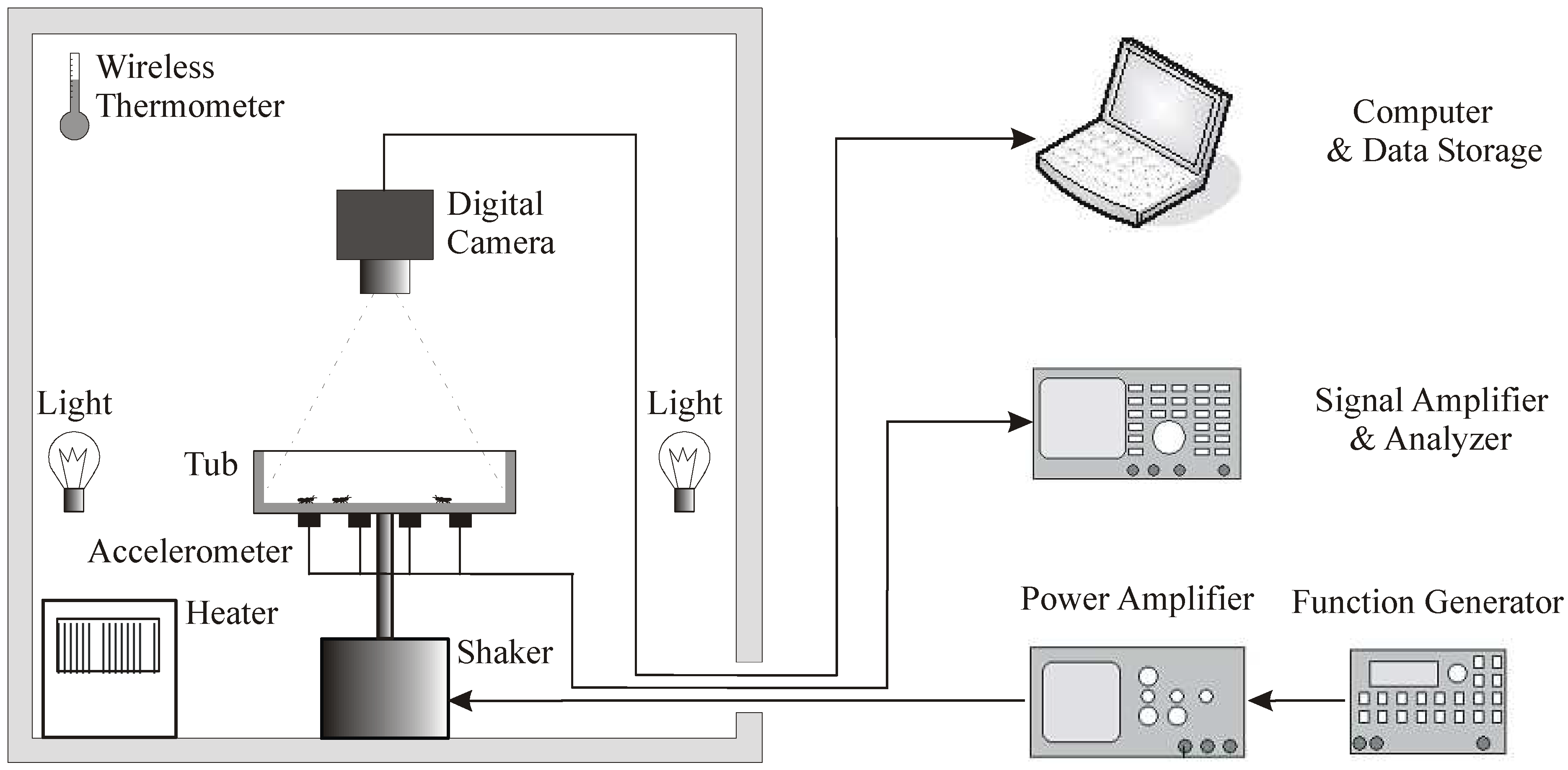
Figure 1.
Schematic illustration of experiment setup for fire ant tracking.
Figure 1.
Schematic illustration of experiment setup for fire ant tracking.
2. Experiment setup
As shown in
Fig.1, a small isolated room measuring about 2×2×2 m
3 was used as the experimental chamber. A small space heater was used to regulate the ambient temperature to 26-28 °C, which was monitored by using a remote wireless thermometer from outside of the chamber. As a play stage for fire ants, a plastic tub measuring 350×190×120 mm
3 was placed in an aluminum support frame, confining the perimeter of the base of the tub but allowing for general deformation of the bottom surface of the tub. The 120-mm sides of the tub were coated with Fluon
® AD1 to prevent the ants from escaping. The 350×190 mm
2 inner bottom of the tub was painted with grid lines of distance of 31.75 mm (1 ¼ inches) for vibration mode analysis and image calibration. Since the vibratory sensory organs of fire ants appear to be most sensitive to the acceleration of the substrate vibration [
15], 12 accelerometers were attached to the outer bottom surface of the tub to monitor the vibration. The tub support frame was connected to the center insert of a shaker by a steel rod. The shaker was placed on a vibration absorbent pad in order to minimize the effects of ambient seismic energy. Four small halogen lamps served as light sources for imaging purposes, and they were placed to prevent shadows. A 10-bit CMOS digital camera with 17-μm pixels was attached to a tripod and fixed to a working distance of 600-mm to capture images of the fire ants before and after excitation. The CMOS camera has a memory big enough to save more than 1,200 frames in each of 10 separate zones, so that image groups of multiple tests can be acquired without pausing for data downloading. The camera acquired image frames of 1024×512 pixels at a frame rate of 60 fps, which covered an area of 418×209 mm
2 in the objective plane with an imaging scale of 2.45 pixel/mm. The exposure time of 1/500 second allowed for sharp images of moving ants.
Other equipment components were placed outside of the room to minimize human interferences with fire ant behavior. The shaker was driven by the output of a power amplifier, and the vibration signals acquired at the tub bottom were amplified using low-noise amplifiers and processed using a dynamic signal analyzer. A computer was used to control the image acquisition and to download images after a test case was completed. Image processing and evaluation were completed offline.
200 workers of fire ants were collected and put into the tub for each test case. Acclimation to the new environment was allowed for 24 hours prior to commencement of experimentation, with drip irrigation providing a source of moisture. Lighting inside the chamber room was regulated by turning the lights on at ~ 8:00 AM every morning and then turning them off at ~ 5:00 PM to simulate the daylight cycle.
According to previous tests [
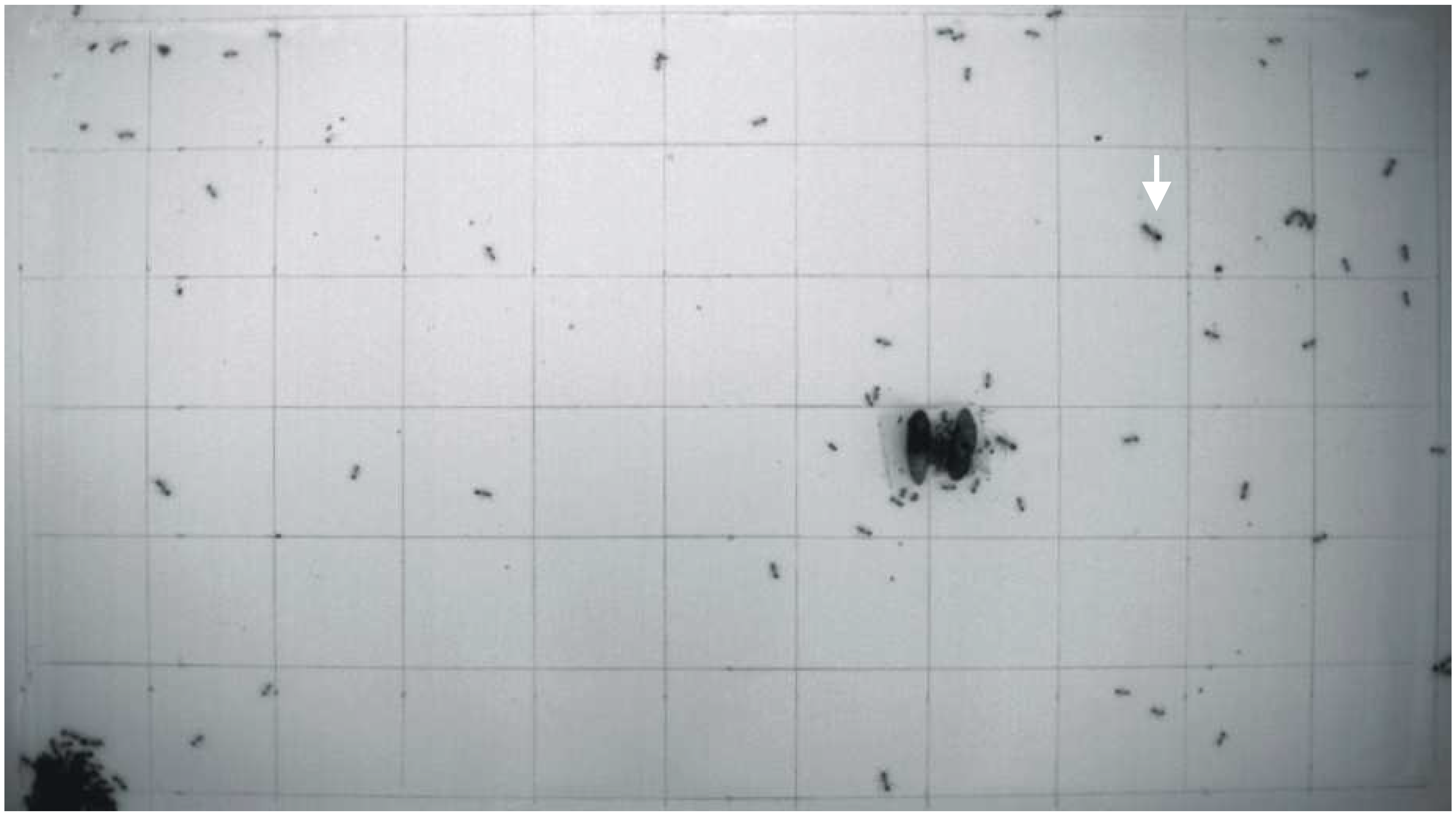
16], the exciting frequency was selected to be 466 Hz to effectively stimulate the fire ants distributed on the tub bottom. Several groups of image frames were recorded for each test case: the first ant image recording group was taken one minute before the excitation as a reference. The second ant image recording group was acquired a few seconds after the ants were excited. The remaining 8 ant image recording groups were obtained at different time delays to observe the development of the ant motion within a one-hour period. Each image group has 1228 frames that were acquired at a rate of 60 fps in about 20 seconds. A sample image is shown in
Fig.2. In this sample image, most of the ants cluster on the lower left corner of the image frame; some of the ants randomly distribute on the tub bottom; and a food source of two
Heliothis virescens pupae is placed on the mid-high right.
Figure 2.
Sample image taken at the bottom of the test tub: fire ants, food source, dusts, grid lines, and shadows are included.
Figure 2.
Sample image taken at the bottom of the test tub: fire ants, food source, dusts, grid lines, and shadows are included.
4. Experiment results
Two tests cases were conducted in two different days and the acquired data provides sufficient information for the test purpose. To effectively stimulate the fire ants distributed on the tub bottom, the exciting frequency was selected to be 466 Hz according to a previous investigation [
16]. The excitation applied in the first case (case #1) resulted in the maximal acceleration amplitude of 0.72 m/s
2 near the tub center, whereas the exciting signal applied in second case (case #2) resulted in the maximal acceleration amplitude of 82.13 m/s
2 at the same position. Therefore, case #1 and case #2 were considered as a weak excitation and a strong excitation, respectively. Since the vibration of the tub bottom surface is perpendicular to the image plane and with limited amplitude, it does not have any obvious influence on the recording of fire ant motion.
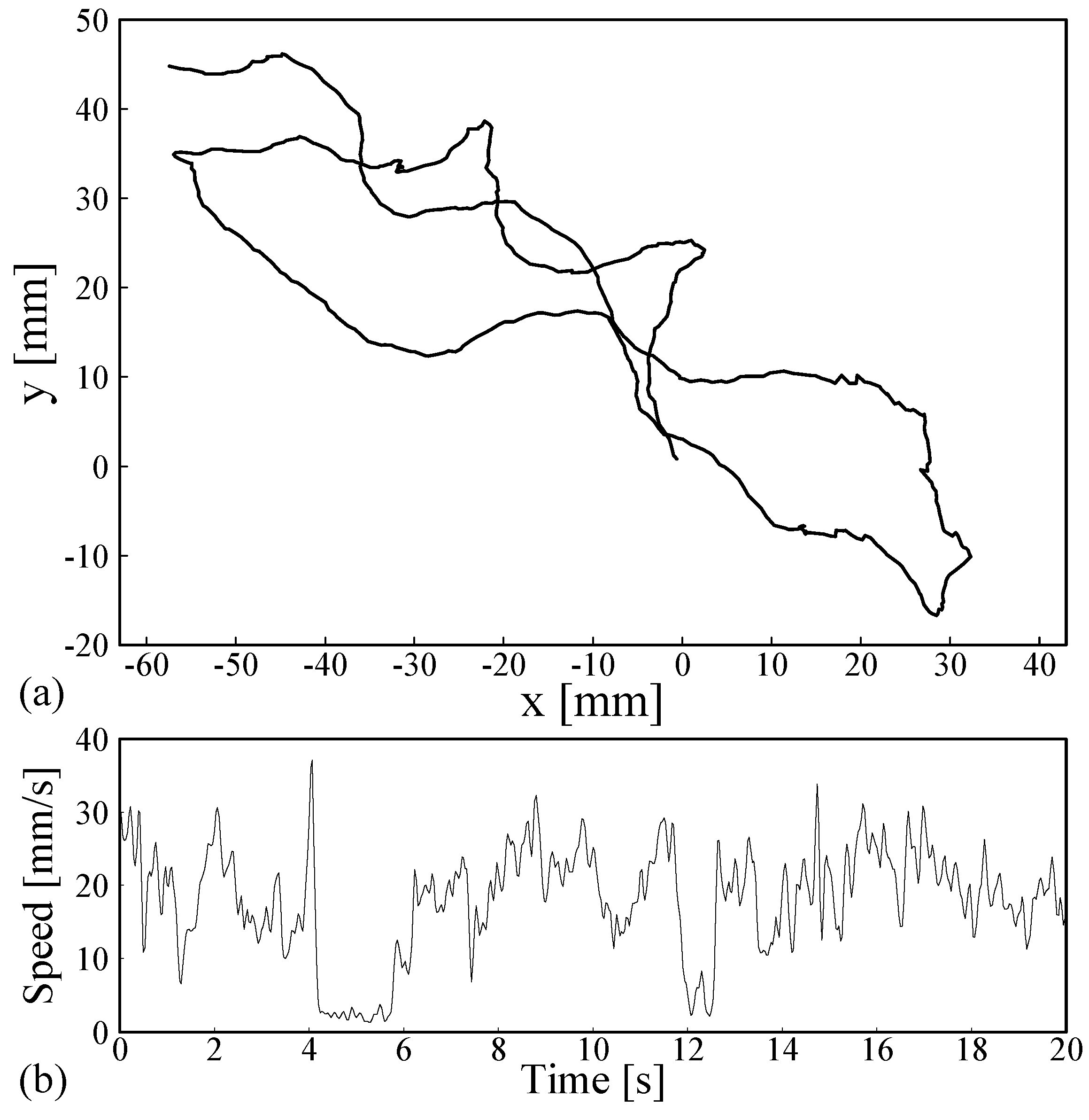
Figure 7.
Individual image tracking results: trail (a) and speed (b) of a selected ant in 20 seconds.
Figure 7.
Individual image tracking results: trail (a) and speed (b) of a selected ant in 20 seconds.
With the described image tracking technique the trail and speed of each active moving ant were determined in a 20-second data acquisition period. As an example,
Fig. 7 shows the trail and speed time history of the ant indicated with a white arrow in
Fig. 2, which belongs to the ant image recording group in case #2 for a few seconds after the excitation.
Fig. 7a shows that the trail of the ant starts at position (0, 0), goes along a “∞” shape in a region of 90×60 mm
2 in the 20-second period. In
Fig. 7b the ant speed varies between 0 and 40 mm/s with a very complex distribution on time. The tracking results for a single ant enable study of the individual ant behavior. However, in the present work we concentrated on the overall behavior of the group of 200 ants.
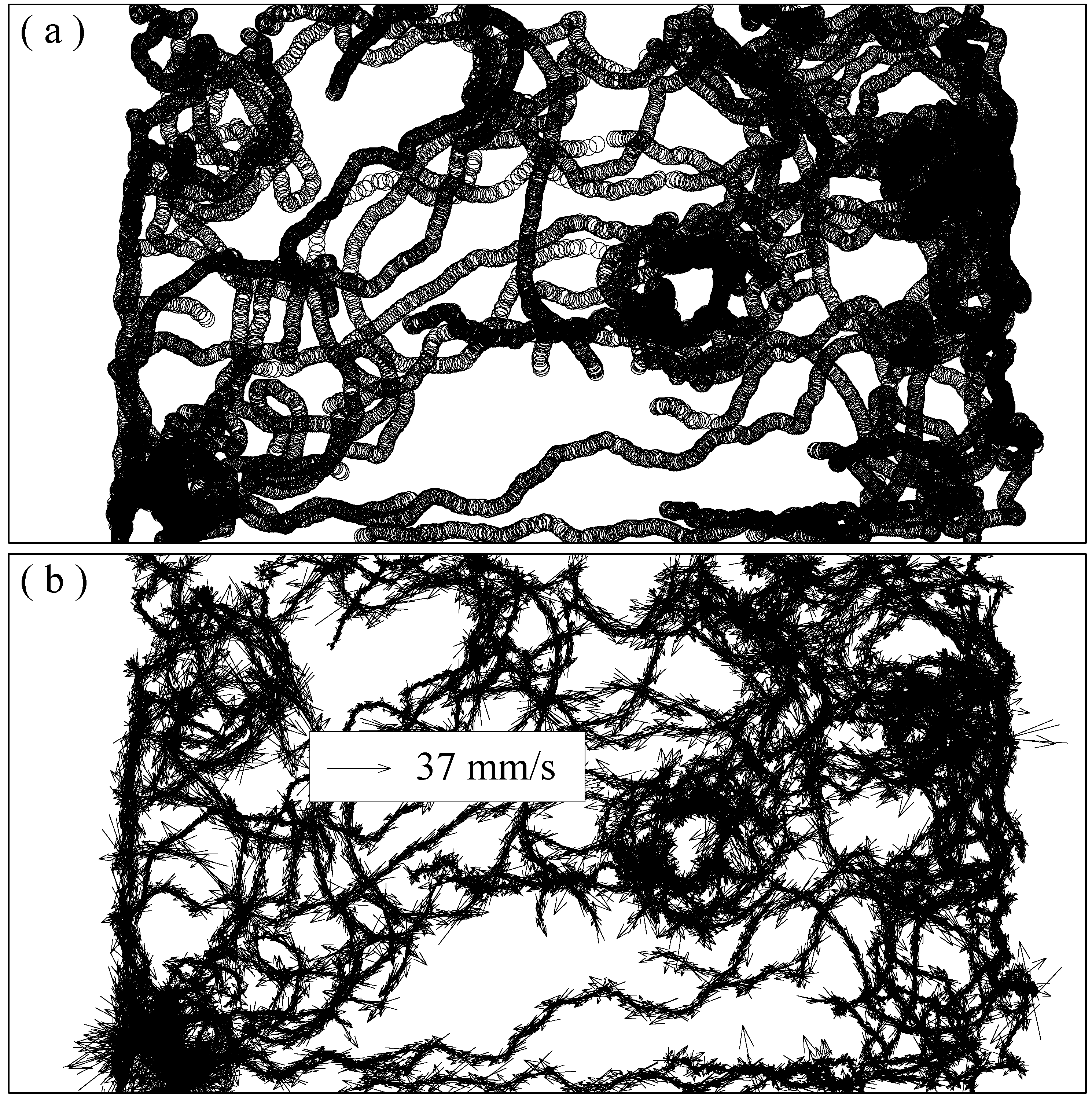
Fig. 8 displays the overlapped positions (8a) and speed vectors (8b) of identified 62 active moving ants in 1228 frames, which are evaluation results of the second ant image recording group for case #2. In
Fig. 8a the trail of an individual ant can hardly be identified, however, the overlapped ant positions present a distribution of ant appearance probability in the observed area.
Fig. 8b shows the corresponding ant moving speed vector at each ant position. Since so many vectors are overlapped, the speed of an individual ant cannot be seen clearly in the figure. In the current test case the constants in Eq. 7 were all set to 1, and those in Eq. 11 were all set to 2.
Figure 8.
Esemble image tracking results: overlapped ant positions (a) and speed vectors (b) in case #2, 2nd group (view area: 418×209 mm2).
Figure 8.
Esemble image tracking results: overlapped ant positions (a) and speed vectors (b) in case #2, 2nd group (view area: 418×209 mm2).
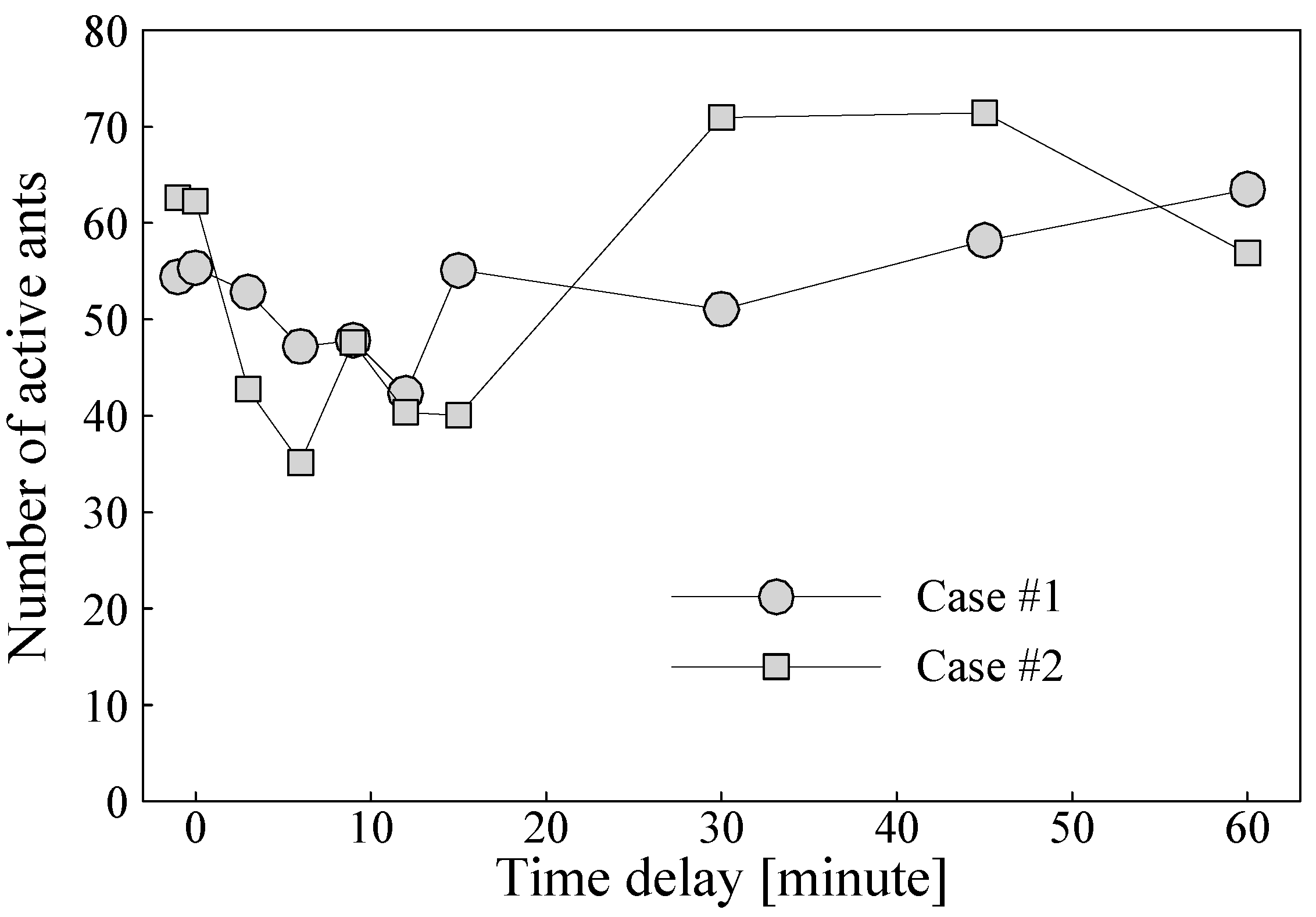
The evaluation results are further processed, so that more useful information can be extracted from the available raw data. At first, the number of the active ants is investigated for the both cases at different delay time in the one-hour test period, and the results are given in
Fig. 9. For each case the first symbol on the left represents the active ant number before excitation, and the second symbol, i.e. at “time delay”=0, represents data obtained a few seconds after the excitation. The followed eight symbols represent data obtained in the time period of restoration, i.e. 3, 6, 9, 12, 15, 30, 45 and 60 minutes after the excitation. As shown in
Fig. 9, test results of both cases indicate that the number of active moving ants reduces after being excited by surface vibration of the tub, and it reaches to the minimum at around 10 minute of the time delay. After 30 minutes, the number of the active moving ants is back to normal, i.e. the number before excitation. After 40 minute the active ant number increases to a little higher than that of before excitation.
Figure 9.
Number of active ants in two test cases during one-hour test period.
Figure 9.
Number of active ants in two test cases during one-hour test period.
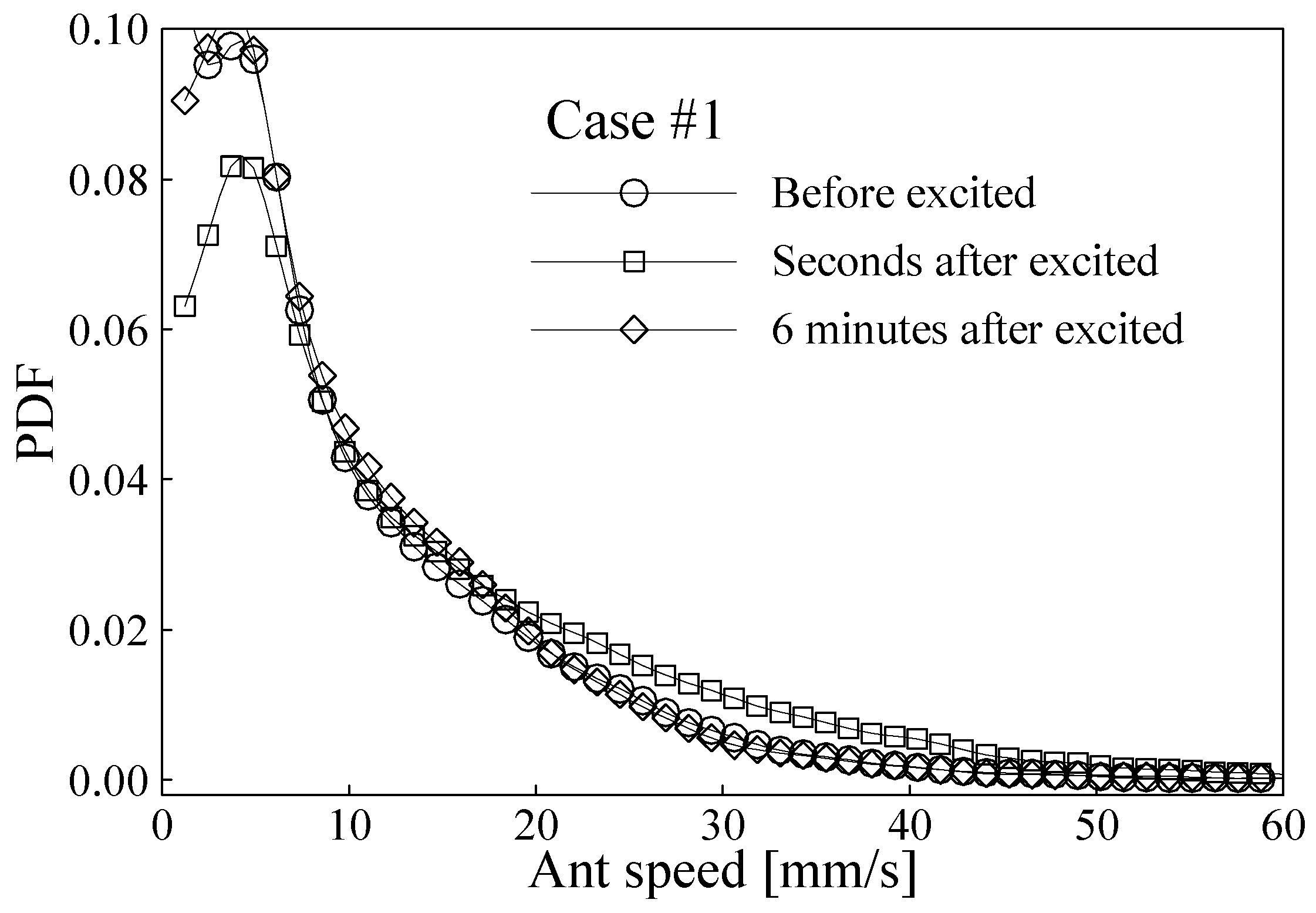
A probability density function (PDF) of ant moving speed is determined for each ant image recording group with about 36000 speed values as shown in
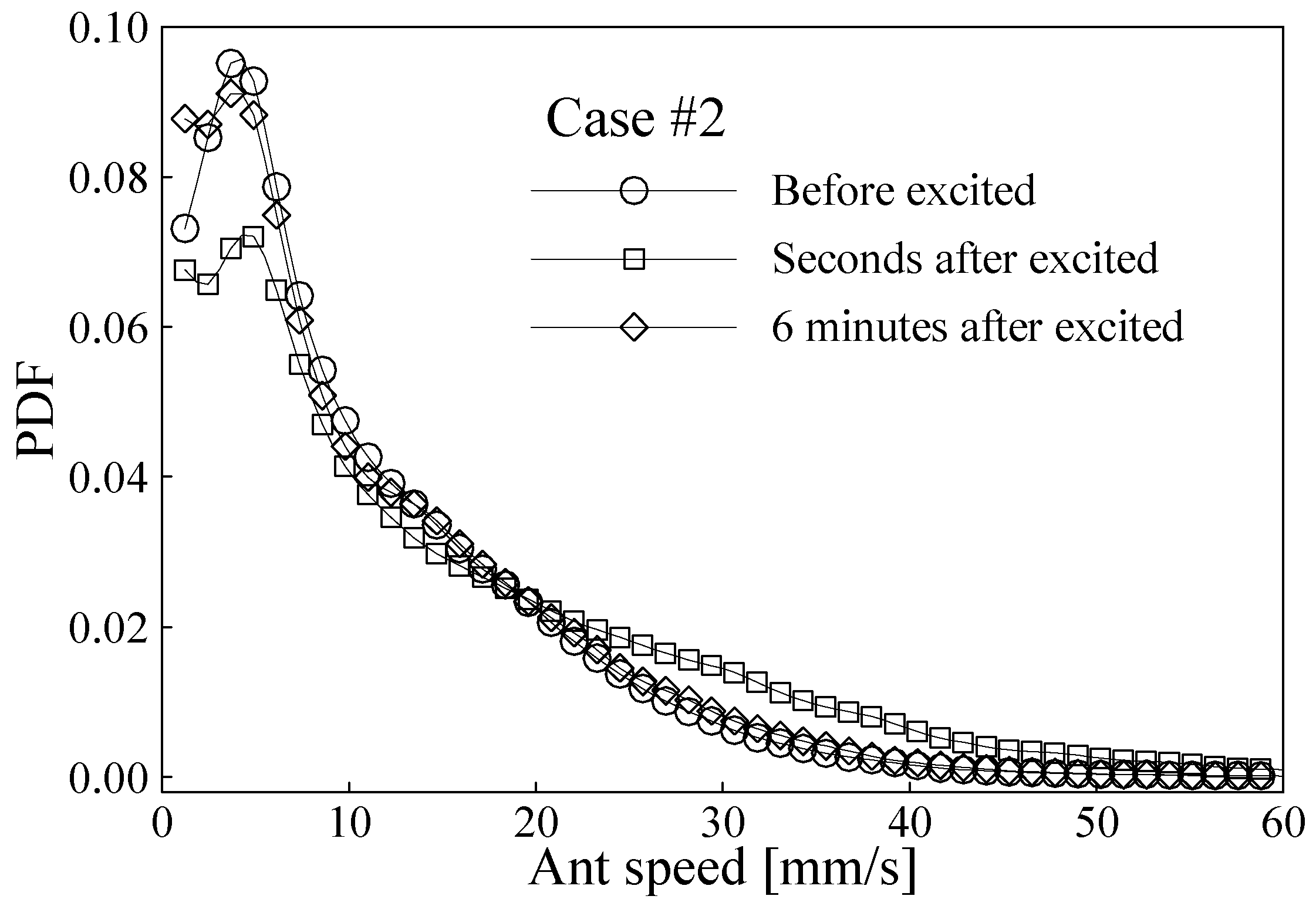
Fig. 8b. The probability density functions (PDFs) of ant speeds determined before excitation, a few seconds after excitation, and 6 minutes after excitation are given in
Fig. 10 and
Fig. 11 for the two test cases, respectively. The PDFs of the two test cases are similar before the ants being excited, and only a little difference can be observed between 10 and 30 mm/s when they are plotted together. The undisturbed PDFs have a maximum near to 5 mm/s, and they reduce exponentially with increasing ant speed. It can be seen in
Fig. 10 and
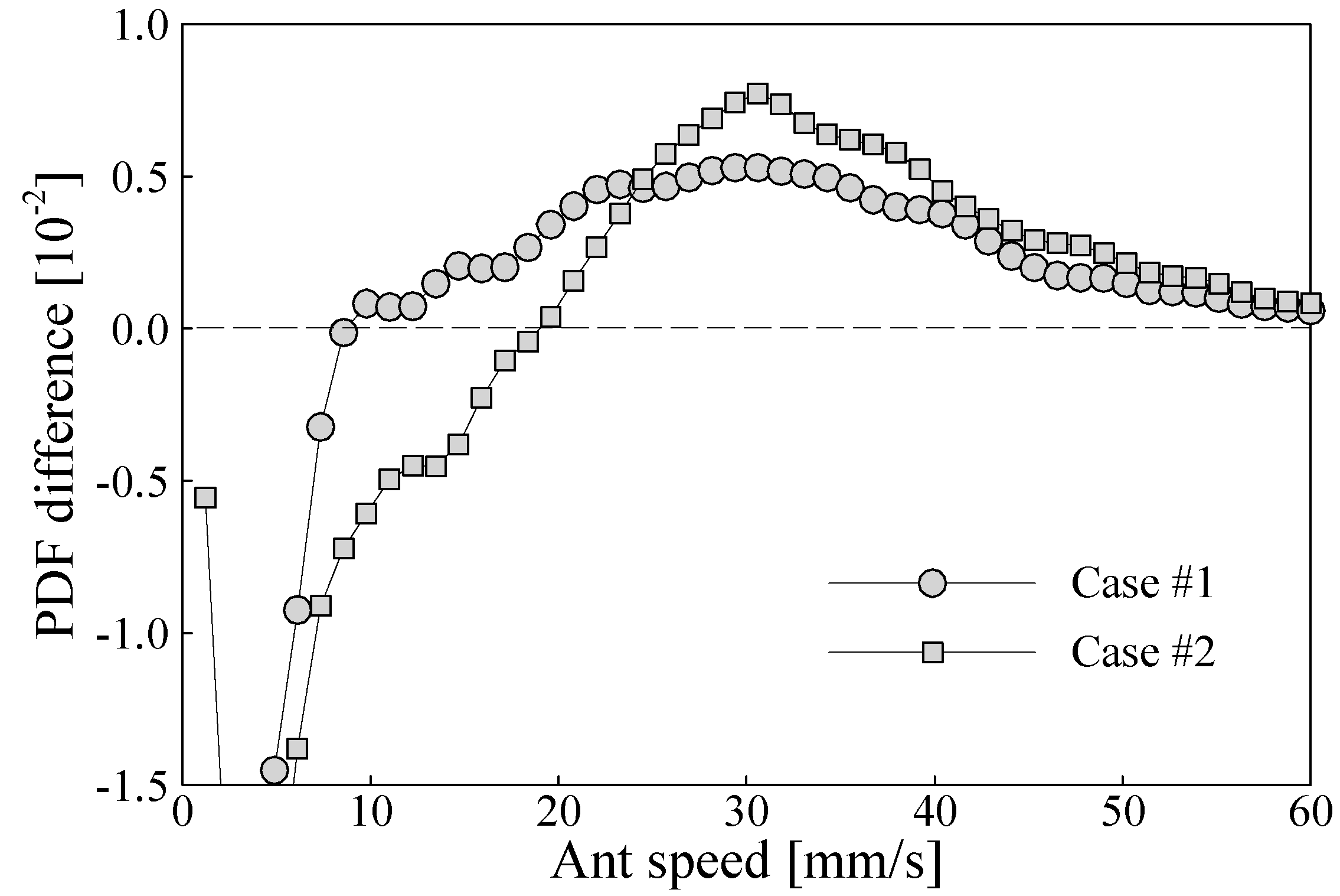
Fig. 11 that the PDF of ant speed is obviously changed in a few seconds after the excitation, but it returns to the undisturbed distribution in about 6 minutes. The excitation of the tub surface vibration reduces the probability density of the low ant speed but increases that of the high ant speed. In order to clearly compare the changes of the PDFs between the two test cases, the PDFs of the undisturbed ant speed are subtracted from the PDFs of the ant speed determined a few seconds after excitation. The differences are shown in
Fig. 12. The figure indicates that the excitation in case #1 increases the PDF of ant speed in the region of more than 10 mm/s, whereas the excitation in case #2 increases the PDF of ant speed for speed more than 20 mm/s. The increasing peak of the PDF is around 30 mm/s for both cases. As a direct consequence of the PDF increasing at the high speed end, the PDF decreases in the region of 0-9 mm/s in case #1 and 0-20 mm/s in case #2. Obviously, the stronger excitation (i.e. in case #2) makes the moving ants a little more active, i.e. at a higher speed level.
Figure 10.
Probability density functions of ant speed for Case #1 at three different test times.
Figure 10.
Probability density functions of ant speed for Case #1 at three different test times.
Figure 11.
Probability density functions of ant speed for Case #2 at three different test times.
Figure 11.
Probability density functions of ant speed for Case #2 at three different test times.
Figure 12.
Probability density function differences in two cases.
Figure 12.
Probability density function differences in two cases.
5. Summary and conclusions
In this paper an image tracking algorithm is used to investigate moving fire ants on a planer surface. The digital images of fire ants are recorded with a high resolution video system, processed to remove the background disturbances, identified with a recursive digital filter, and tracked with their position, size, brightness, shape and orientation angles.
The fire ant image tracking is conducted in two ways, i.e. individual image tracking and ensemble image tracking. The individual image tracking is started with a selected fire ant at the first frame of a successively recorded image group. The selected fire ant image is tracked from frame to frame until it stops or goes out of the image frame. Since the individual fire ant image tracking may fail when two or more fire ants meet together, the tracked trail should be confirmed with a video playback. If the individual fire ant tracking is successfully completed, a position time history of the selected fire ant is determined and the speed variation can be investigated. The ensemble image tracking can be conducted with a minimum of two frames, and the speed values of a group of fire ants are determined for statistical analysis.
Tests were conducted with a group of 200 fire ant workers in a plastic tub. The test fire ants were excited with tub surface vibration of selected frequency and intensity. The experiment shows that, after acclimation to the environment for 24 hours, around three quarters of the ants keep calm in clusters, whereas about one quarter of the ants move actively. The speed of the active moving fire ants increases directly after the excitation, and return back to the normal level in about 6 minutes. The ant speed level is a little higher after a strong excitation than after a weak excitation. Experiment results indicate that the number of the active moving ants does not increase as expected after the excitation with substrate vibration, in the contrary, it decreases within 10 to 20 minutes after the excitation.
The application example demonstrates that the image tracking algorithm, which was originally described for tracking big buoyant particles in a water tank, can be effectively used to track images of moving fire ants on a planar surface with a necessary modification, i.e. including the orientation angle in the tracking function. The background image removing erases not only disturbances in the image background, but also images of fire ants that do not move, so that the active moving fire ants can be counted precisely. The used image identification method is effective but simple, so that it can easily be put into a computer program. The presented algorithm and method may be further improved with recent advancements in particle image velocimetry, e.g. [
17,
18], and used to track other insects moving on a planar surface.


