Due to its peculiar features, before proceeding with the compressive characterization of foam specimens, the MHPB-SM requires a series of experimental steps to tune the data elaboration procedures in order to achieve optimized results. First, it is essential to verify the strain measurement chain with regards to repeatability, accuracy, and linearity. This check is performed statically in terms of force using a reference load cell placed between the input and the output bars and compressing them with the pre-stressing actuator. All the strain-gage measurement points and the reference load cell are in series and they must measure the same force (except for the friction between the bars and the Teflon bushings).
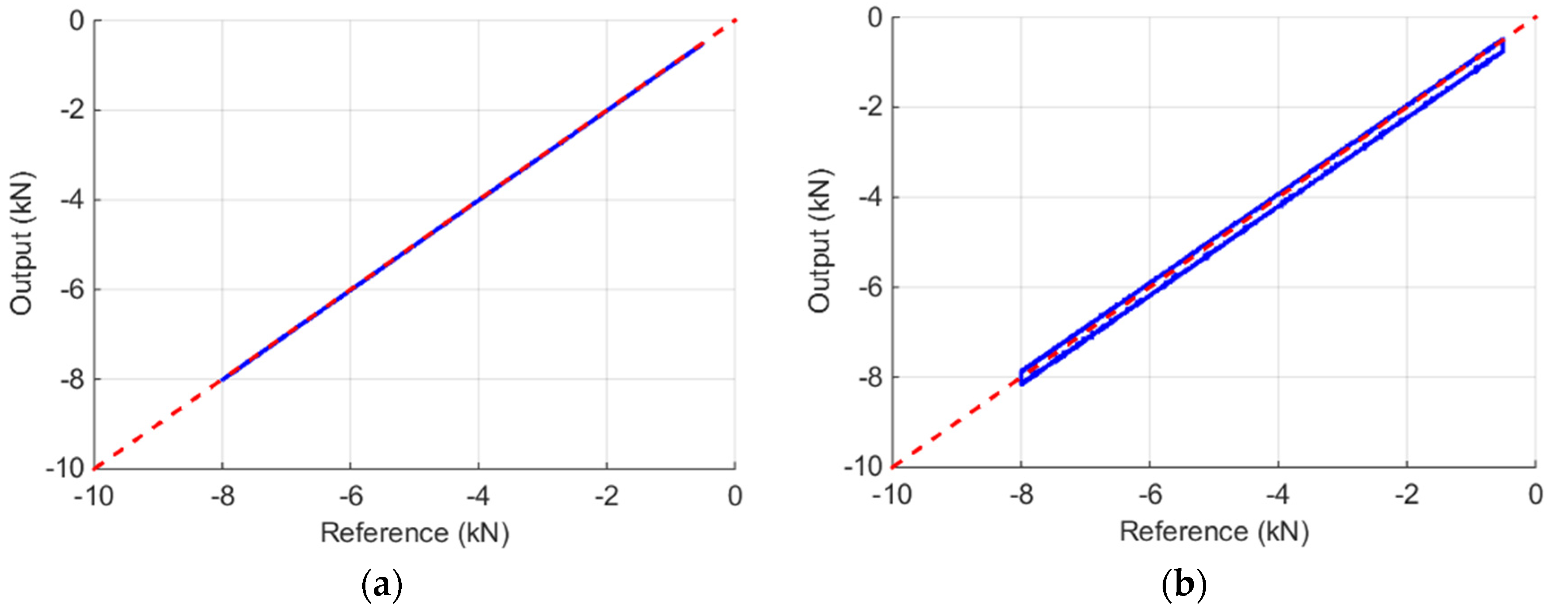
Figure 4 shows the calibration curves for two measurement points on the apparatus bars.
Figure 4a displays three consecutive loading and unloading paths recorded at one of the measurement points (
Ainput) on the instrumented input bar segment farther away from the specimen. As can be seen, in the tested force range there is no non-linearity present, and friction phenomena are negligible. However, in the data obtained from a measurement point placed near the pre-stressing jack (
Figure 4b) friction is present. It is quantifiable to approximately 0.3 kN in the calibration range and it is due to the 30 supports between the reference load cell and the measurement point. This fact further justifies the instrumentation of the bar segments in the proximity of the specimen. In addition, in the calibration step it is possible to verify and, if necessary, adjust with a correction coefficient the experimental results in order to ensure the same sensitivity for all measurement points (different sensitivities occur due to strain-gage misalignments or different amplifier gains).
Figure 4.
Calibration of measurement point on: (a) the instrumented bar segment (measurement point Ainput); and (b) in the proximity of the pre-stressing jack (measurement point D).
Finally, it must be underlined that, the MHPB-SM has the additional advantage, compared with other Hopkinson-bar based apparatuses, to be easily calibrated using the pre-stressing jack already mounted. In fact, for the calibration, it is not as simple to load all the bar strain transducers simultaneously by generating the compression pulse with an impacting striker bar in the SHPB [
22] or by using the tensile pre-tensioning method adopted in [
23]. A robust calibration procedure is an essential requirement to ISO 9001 quality standard [
24] of a modern material testing equipment.
3.1. Void Test
The next essential step towards “tuning” the data elaboration procedure in order to enhance the accuracy of the data analysis is the so-called “void test”: in practice, the input and output bars are brought in contact, a compression test without a specimen is performed, and the forces and displacements at the input-output bar interfaces are reconstructed and compared. This test can be considered as representing a well-known boundary condition problem, and is in particular useful for tuning some stabilization coefficients of the wave separation algorithm proposed in reference [
18].
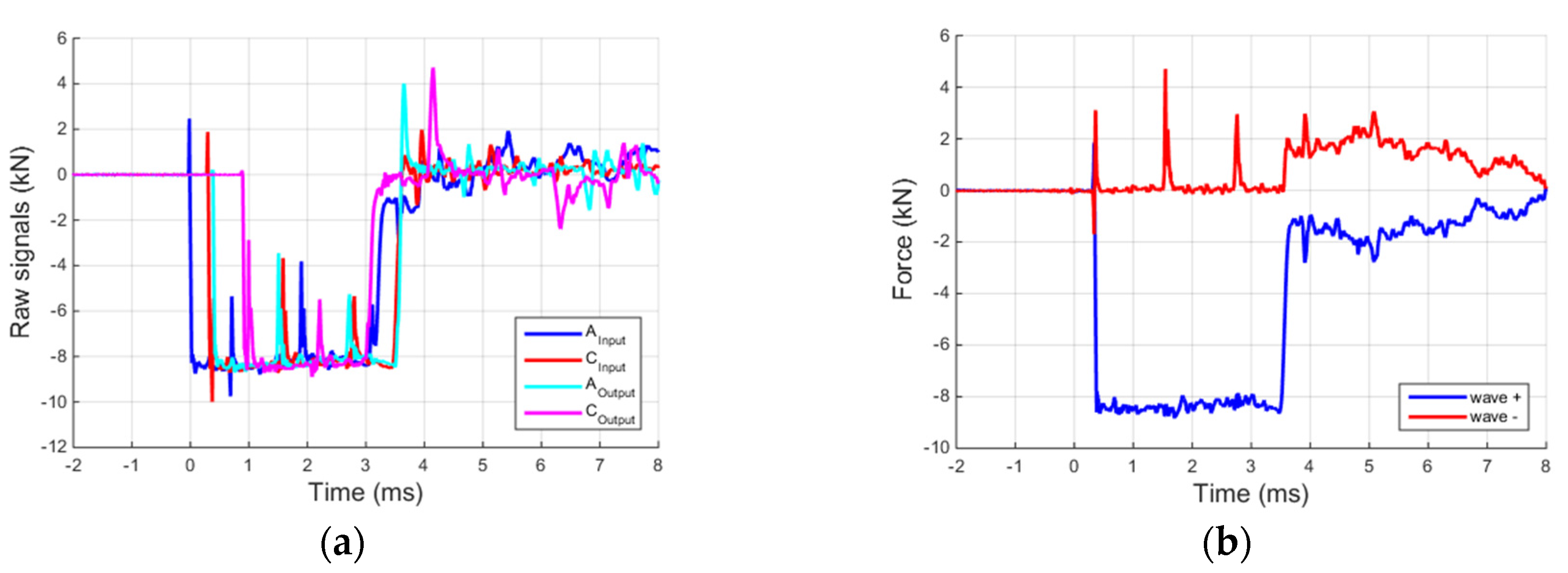
As mentioned in the previous paragraph, starting from at least two strain-histories recorded in different locations on a single bar (
Figure 5a) it is possible to reconstruct the ascending and descending waves in any other bar location using the deconvolution algorithm [
19]. The algorithm uses the theoretical three-dimensional wave propagation theory in infinite elastic rods (Pochhammer-Chree theory), and works in the frequency domain. It further requires the prior determination of some stabilization coefficients, which is accomplished by using the recorded data sets mentioned above.
Figure 5b shows the results for the input bar and in particular the ascending (wave +) and descending waves (wave −), respectively, at the input-output bar interface. The adopted algorithm has the advantage of working on the entire time domain and of directly applying the correct time shift to the reconstructed waves. As seen in
Figure 5b, the algorithm is also able to satisfactorily identify spurious reflections due to the small impedance mismatch at the input-output bar interface (first peak on the reflected wave) or at the bar sleeve-joints (second and third peak on the reflected wave).
Figure 5.
(a) Raw signals recorded on the Input and Output bars on two locations; and (b) wave propagating in the input bar reconstructed at the input–output bar interface.
Figure 5.
(a) Raw signals recorded on the Input and Output bars on two locations; and (b) wave propagating in the input bar reconstructed at the input–output bar interface.
At this point, by applying the well-known Hopkinson bar formulae, the forces and displacements of the two bars at their interface can be reconstructed, as shown in
Figure 6. In particular, the forces at a bar interfaces are proportional to the sum of the two ascending and descending waves previously computed, whereas the displacements are proportional to the difference of the same waves.
Figure 6a presents the equilibrium check at the input-output bar interface in the time domain, and the excellent quality of the results is to be attributed to the previous calibration and the precision tuning of the stabilization coefficients of the separation algorithm. With reference to
Figure 6, it can be noted that the two bars remain in contact for about 3.2 ms (the duration of the input pulse) and then the output bar moves away from the input bar (and the interaction force drops to zero).
Figure 6b shows the comparison between the input and output bar end displacements obtained with the Hopkinson bar theory and with the fast tracking optical algorithm, described in the previous paragraph. To analytically evaluate the differences between the curves reported in
Figure 6b (two “Hopkinson” and two “optical” displacement data series) the relative error is determined, defined as:
where DHopkinson and DOptical are, respectively, the bar end displacements obtained with the advanced Hopkinson elaboration and the optical algorithms, previously mentioned. This index can be thought as representing the mean error divided by the reference mean displacement. Relative errors of 0.88% and 0.22% have been computed for the input and the output bars, respectively.
Figure 6.
(a) Equilibrium check at input-output bar interface; and (b) comparison between displacements obtained with Hopkinson bar theory and with the fast tracking optical algorithm.
Figure 6.
(a) Equilibrium check at input-output bar interface; and (b) comparison between displacements obtained with Hopkinson bar theory and with the fast tracking optical algorithm.
The optical displacement reported in the graph is the average displacement of the targets adjacent to bar interface (targets 5,6 for the input bar and 7,8 for the output bar). The three curves of
Figure 6b, based on two independent measurement data sets, are practically coinciding up to about 4 ms, thus demonstrating once again the accuracy of the data processing implemented. After the detachment of the two bars, some oscillations reduce the accuracy of the Hopkinson bar elaboration (especially for the input bar). However, this can be readily identified and controlled thanks to the high-speed camera measurements, and in no way would it influence the outcome of compression tests (already completed by that time).
3.2. Foam Tests
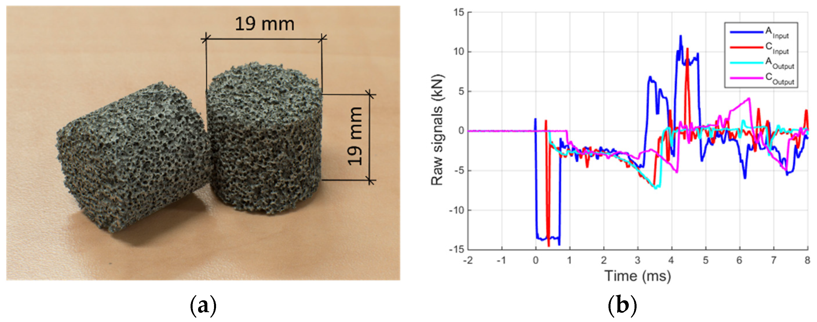
Following the static calibration of the strain transducers and the dynamic tuning of separation algorithm achieved with the void test, it is straightforward to apply the MHPB-SM technique to an actual compression test on foamed material. A series of such compression tests have been performed on cylindrical specimens with a diameter of 19 mm and a length of 19 mm (
Figure 7a).
The specimens have been cut using electrical discharge machining from a block of ALUHAB aluminum foam with a density of about 0.55 g/cm3 and an average pore size of 1 mm, manufactured by Aluinvent. This cell size renders the specimen of 19 mm size suitable for the characterization of the foam with the MHPB-SM, as it constitutes a representative volume of the material. The ALUHAB aluminum foam comes under the market name of EN43100 8ALO2, which is manufactured from the aluminum alloy EN43100 (AlSi10Mg base) and where 8ALO2 means 8% in volume of Al2O3 particles of 2 microns. The technology uses special high temperature admixing to homogeneously disperse the particles and thus creates a stable, foamable aluminum melt. This technology permits the injection of optimally sized bubbles from 10 to 0.5 mm range into the melt.
Figure 7.
(a) Specimen of aluminum foam ALUHAB; and (b) raw signals recorded on the input and output bars on two locations.
Figure 7.
(a) Specimen of aluminum foam ALUHAB; and (b) raw signals recorded on the input and output bars on two locations.
As in the void test, the raw signals recorded during the material tests are totally overlapped for both input and output bars, as shown in
Figure 7b. Applying the separation algorithm on the two data series related, respectively, to the input and output bars, the ascending and descending waves are accurately reconstructed,
Figure 8.
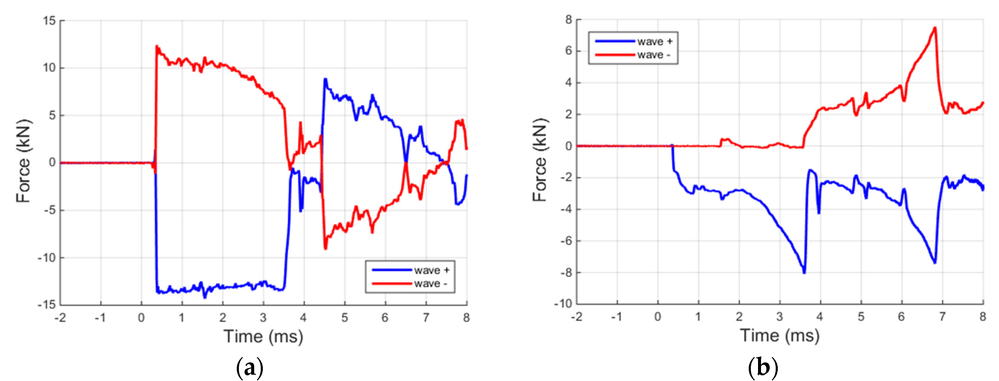
Figure 8a shows clearly the rectangular incident and the reflected waves. After about 4 ms, the reflected wave comes back to the bar end (previously in contact with the specimen) and continues to travel inside the input/pre-stressed bar generating the strange wave tails. On the other hand,
Figure 8b shows the two waves travelling in the output bar. For about 3.2 ms the ascending wave is practically equal to the force applied to the specimen except for the small reflections due to the bar joints (small oscillations of the descending wave in the initial 3.2 ms).
Figure 8.
Waves propagating in the (a) input; and (b) output bars, reconstructed at the interfaces with the specimen.
Figure 8.
Waves propagating in the (a) input; and (b) output bars, reconstructed at the interfaces with the specimen.
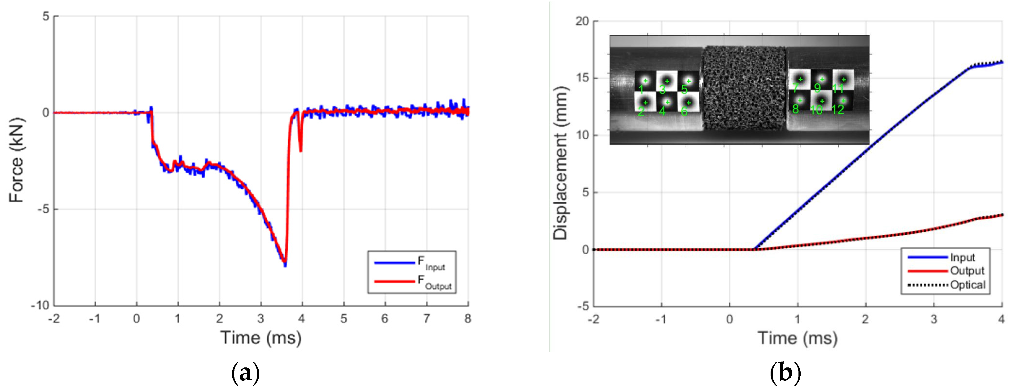
At this point, the forces and displacements applied to the two faces of the specimen can be determined. In this way, the specimen force equilibrium is checked and successfully verified, as shown in
Figure 9a. It is interesting to underline that in all graphs presented no other filtering has been applied in order to be able to focus on and assess only the performance of the equipment and the data elaboration procedure. Although the input force is noisier compared with the output one (which is naturally filtered by the specimen mass and damping), the specimen equilibrium is attained even when the specimen is crossed by the ascending profile of the compression pulse. For what concerns the displacements, also in this case, there is an excellent agreement between the data derived from the strain-gage measurements and those of the high-speed photo sequence (
Figure 9b). The absence of delays between the two data series once again validates the effectiveness of the applied data elaboration. The relative errors computed using Equation (1) are, respectively, 0.88% and 1.03% for the input and the output bar.
Figure 9.
(a) Equilibrium check at specimen-bars interfaces; and (b) comparison between displacements obtained with Hopkinson bar theory and with the fast tracking optical algorithm.
Figure 9.
(a) Equilibrium check at specimen-bars interfaces; and (b) comparison between displacements obtained with Hopkinson bar theory and with the fast tracking optical algorithm.
Based on the above and the hypothesis of uniform stress-strain fields in the specimen below, the histories of stress
σ, strain-rate
, and strain
ε of the specimen can be written using the standard Hopkinson bar relationships:
where,
F and
v are, respectively, the forces applied and the velocities at the two specimen surfaces (
i = input,
o = output);
Ab and
As the bar and the specimen cross-sections;
L the specimen length; and
ε+ and
ε− are respectively the ascending and descending strain waves reconstructed at the specimen-bar interfaces (
i = input,
o = output), derived from
Figure 8.
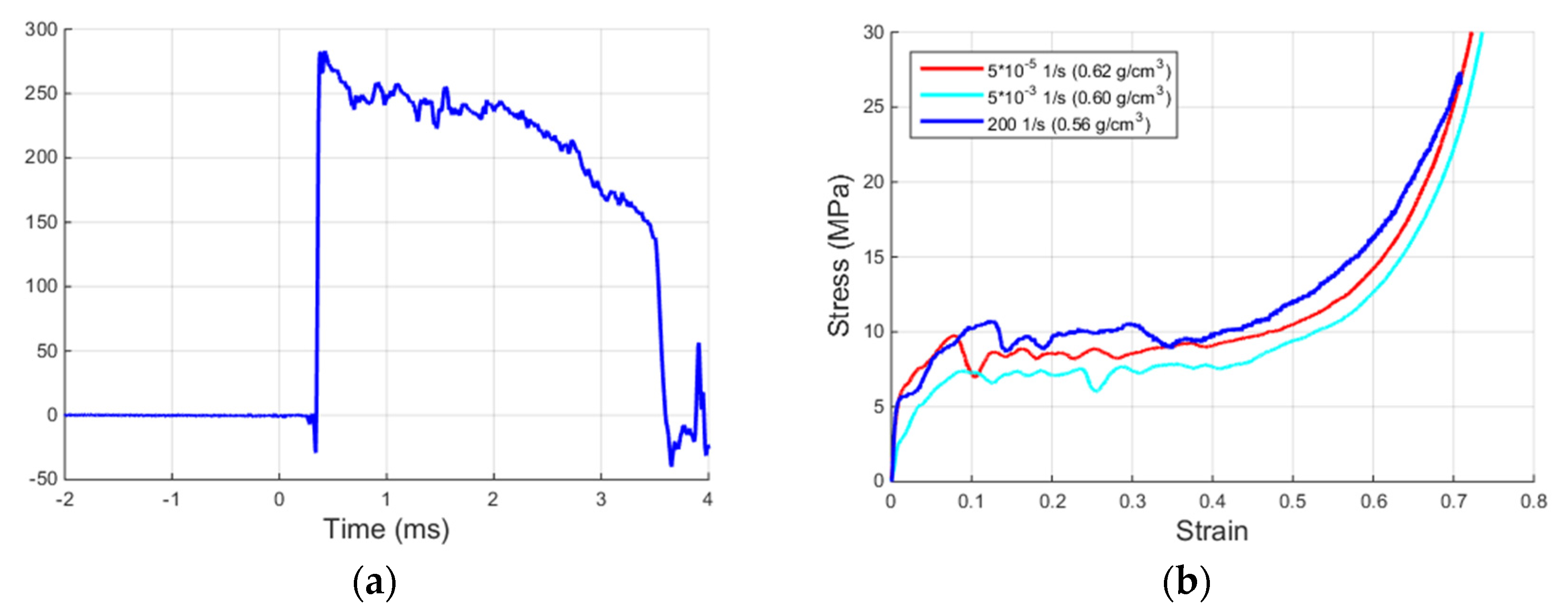
The two graphs in
Figure 10 show the specimen strain-rate during a MHPB-SM test and the specimen stress-strain curve obtained using relations Equations (2)–(4). It is observed that, thanks to the characteristic, well-pronounced plateau in the stress-strain curve, the test is performed at an almost constant strain-rate of approximately 200 s
−1. This aspect is important if the material strain-rate sensitivity is to be investigated; clearly, other strain-rates can be produced by changing the initial compression force in the pre-stressed bar and/or by varying the length of the specimen. Concerning the apparatus limits in the current configuration, it is evident that they are connected to the magnitude of the compressive force in the pre-stressed part. This force must be such that the bar remains always elastic, it must be less than the buckling load, and it must not exceed the capacity of the clamp/release mechanism. Specifically, a pre-stress between 15 and 40 kN can be easily applied, which would correspond, respectively, to a specimen strain-rate between 100 and 400 1/s (assuming the same specimen strength). By halving the specimen length (and still maintaining a representative material volume), these strain-rate values would be almost doubled, as Equation (3) indicates. Also for the same specimen length, larger pre-loads would produce larger maximum deformations (full densification with 40 kN pre-stress and only part of it with 15 kN pre-stress).
With reference to the stress-strain curve of
Figure 10b, it is noticed that the strain reached when using a specimen of larger dimensions (than that for metals or plastics of the standard SHPB) is more than 70%. This feature allows an effective characterization of the stress-strain curve of foamed and, in general, soft materials. In fact, apart from the stress plateau, which is entirely reproduced, even the onset of the specimen densification phase is well captured. A shorter specimen would have allowed its full reproduction. For comparison purposes, two low strain-rate stress-strain curves of this foam (obtained with a servo-hydraulic universal testing machine) are also included in
Figure 10b. For the strain-rate range considered, the strain-rate sensitivity appears to be negligible, especially when compared with the natural data scattering of this type of material.
Figure 10.
(a) Specimen strain-rate during a MHPB-SM test; and (b) engineering stress-strain curve of ALUHAB foam.
Figure 10.
(a) Specimen strain-rate during a MHPB-SM test; and (b) engineering stress-strain curve of ALUHAB foam.
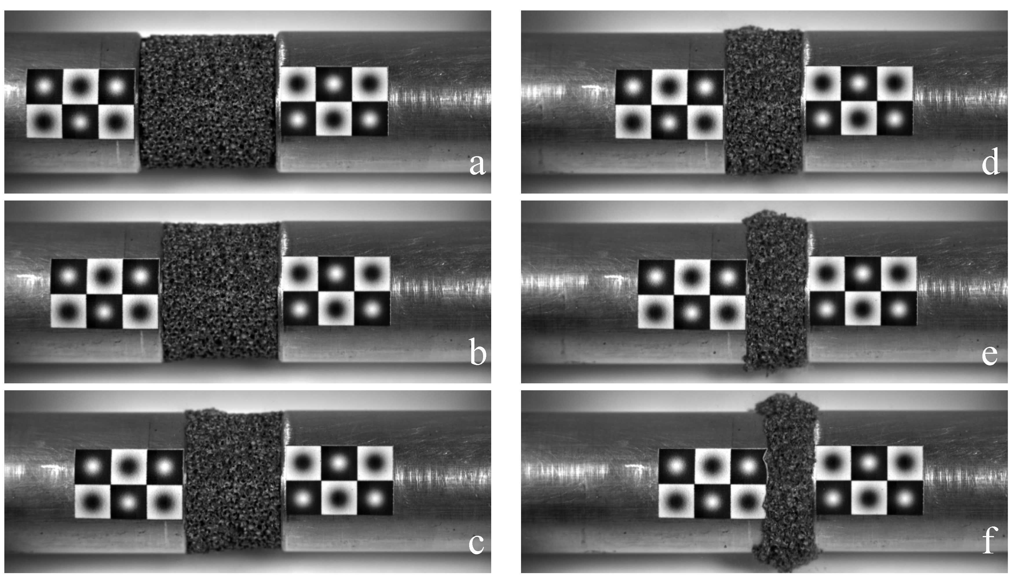
Finally,
Figure 11 shows an example of a series of a high-speed photo sequence frames recorded during a MHPB-SM test on an aluminum foam specimen. As mentioned before, in addition to the fast tracking algorithm useful to measure the bar’s displacements, it is possible to apply the optical flow method to evaluate the displacements and eventually the strain field of the specimen during the test. This type of analysis provides the possibility to study the collapse mechanism of a foamed material and to check the existence of peculiar instability phenomena that can occur under dynamic conditions.
Figure 11.
High-speed photo sequence of a MHPB-SM test: (a) 0.36 ms; (b) 1.00 ms; (c) 1.64 ms; (d) 2.28 ms; (e) 2.92 ms; (f) 3.56 ms.
Figure 11.
High-speed photo sequence of a MHPB-SM test: (a) 0.36 ms; (b) 1.00 ms; (c) 1.64 ms; (d) 2.28 ms; (e) 2.92 ms; (f) 3.56 ms.


