The Nature-Inspired Metaheuristic Method for Predicting the Creep Strain of Green Concrete Containing Ground Granulated Blast Furnace Slag


Abstract
:1. Introduction
2. Experimental Setup
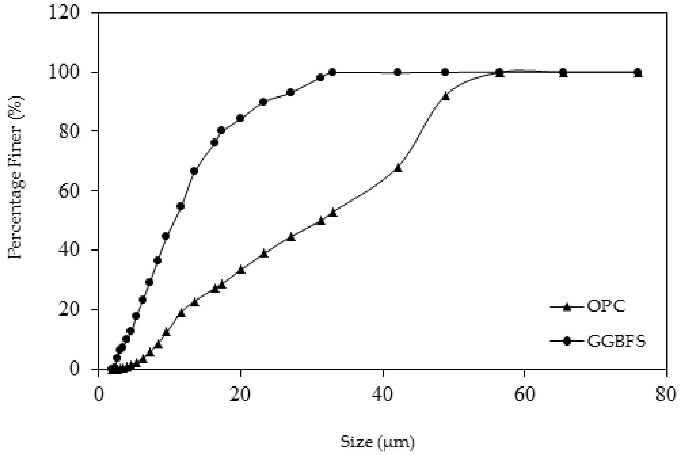
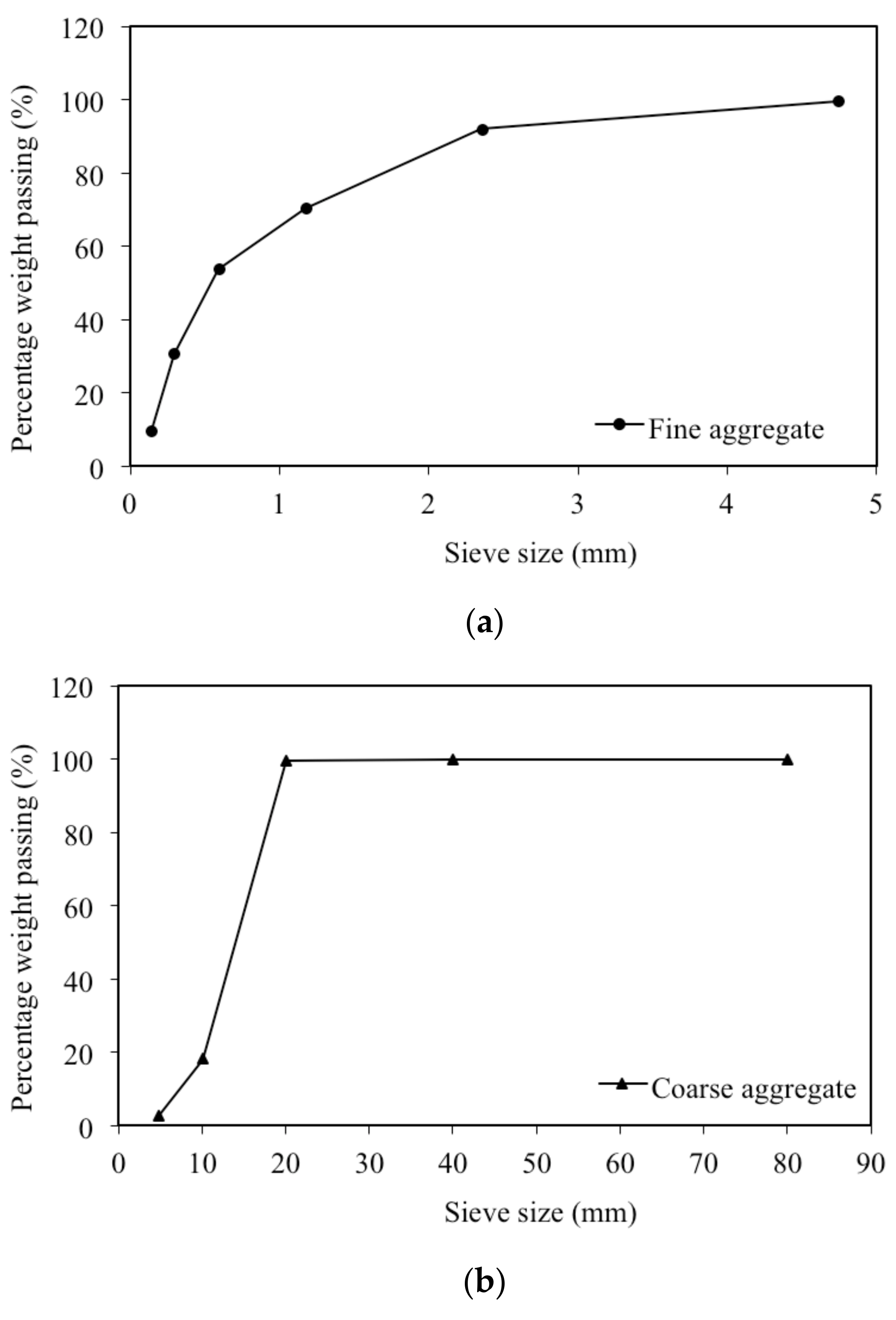
2.1. Materials
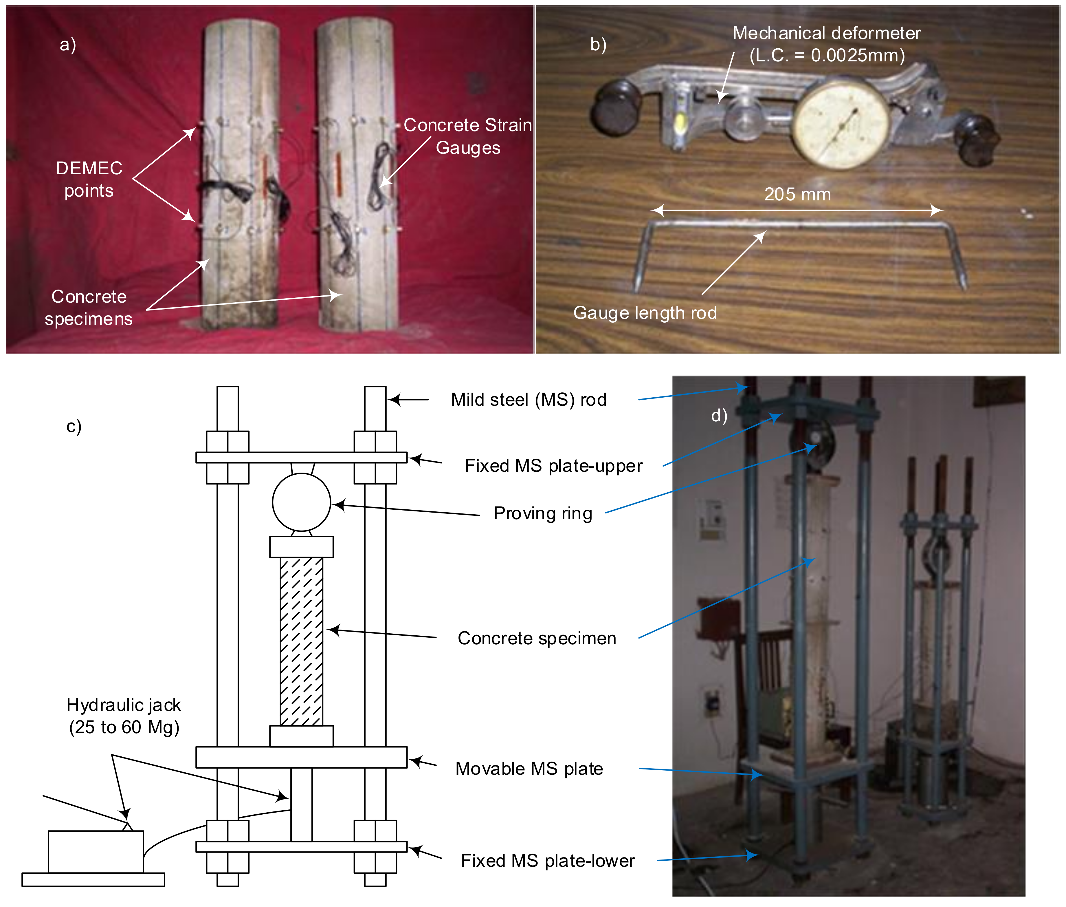
2.2. Methods
2.3. Statistical Analysis of the Database
3. Numerical Analysis
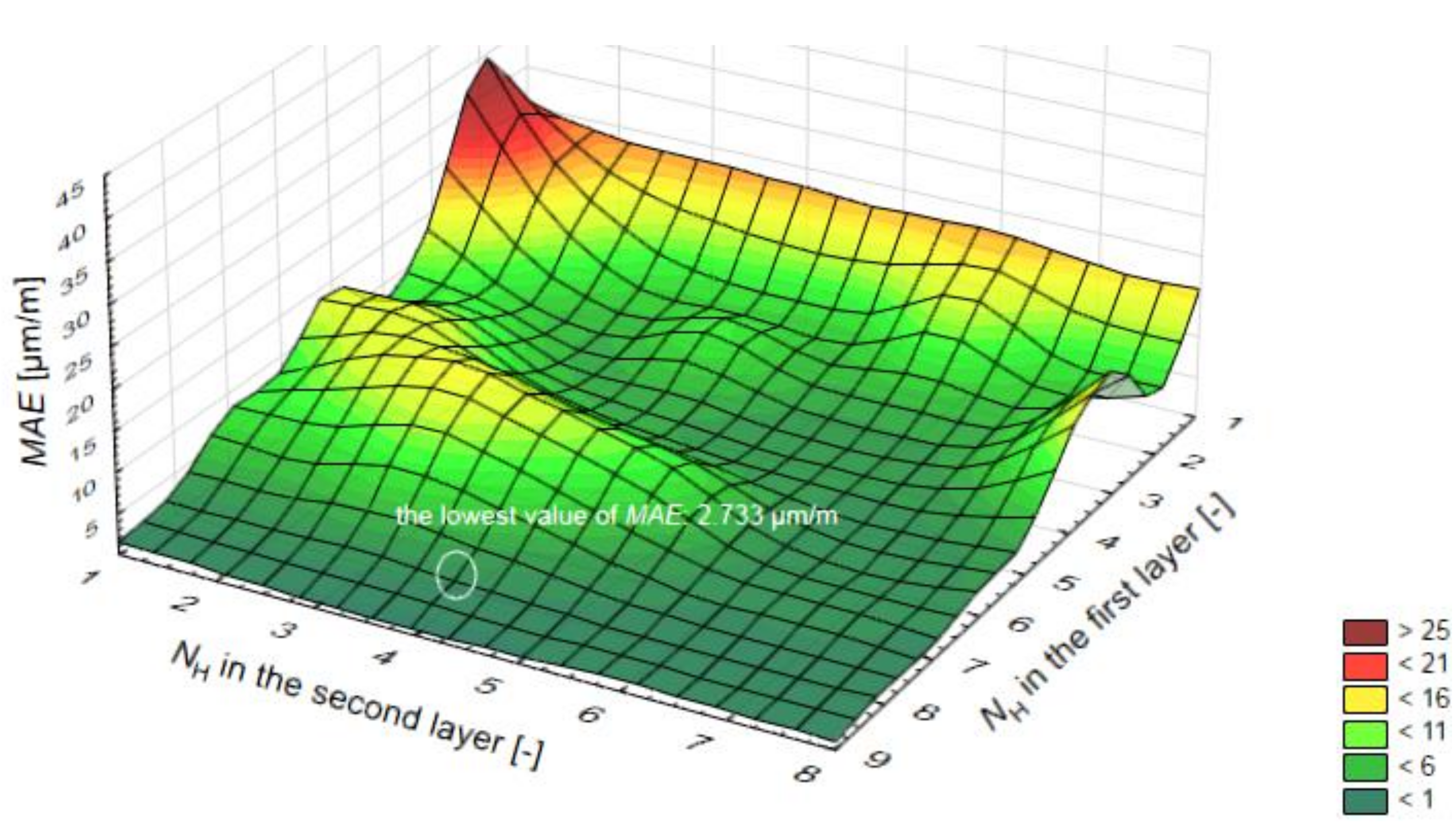
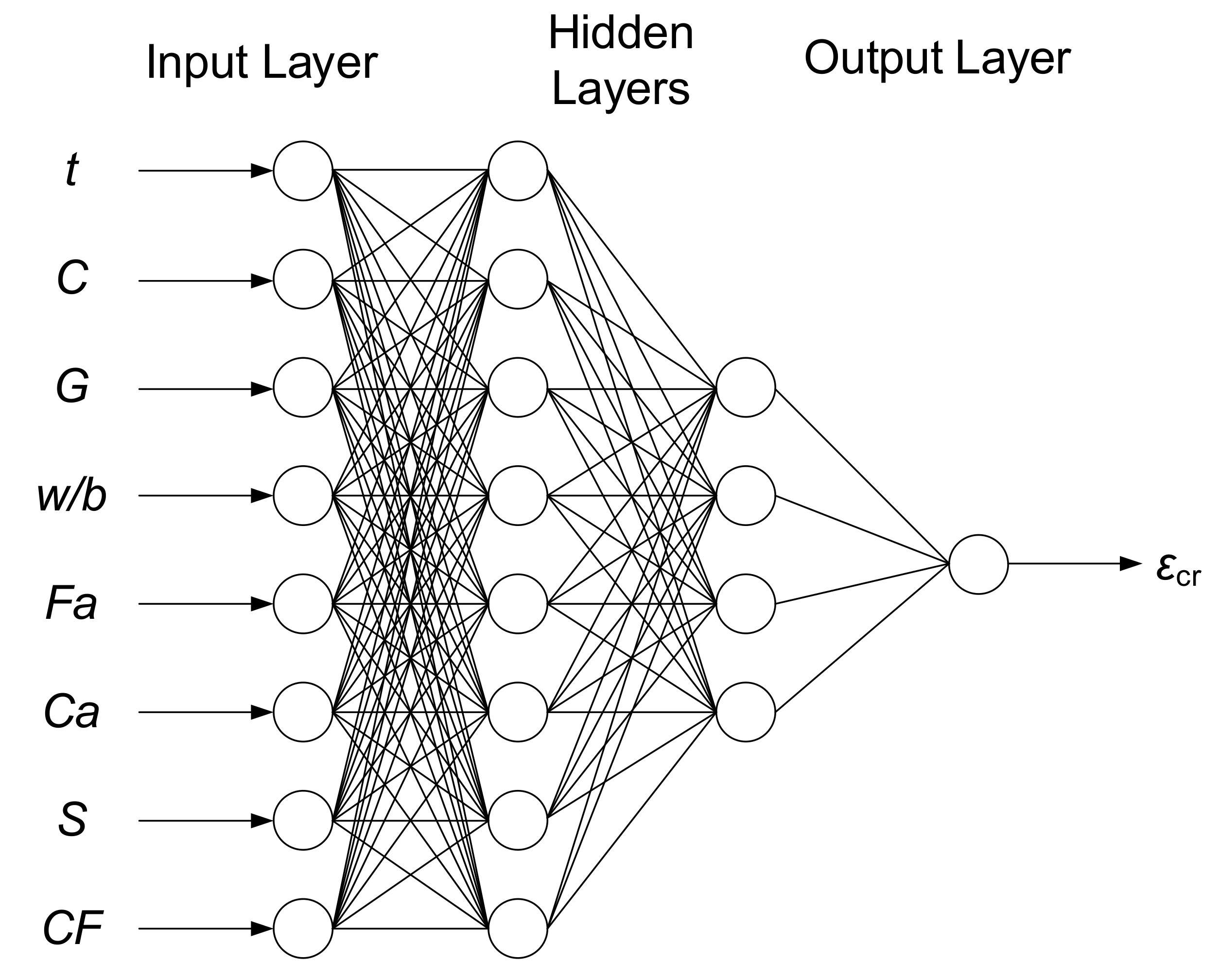
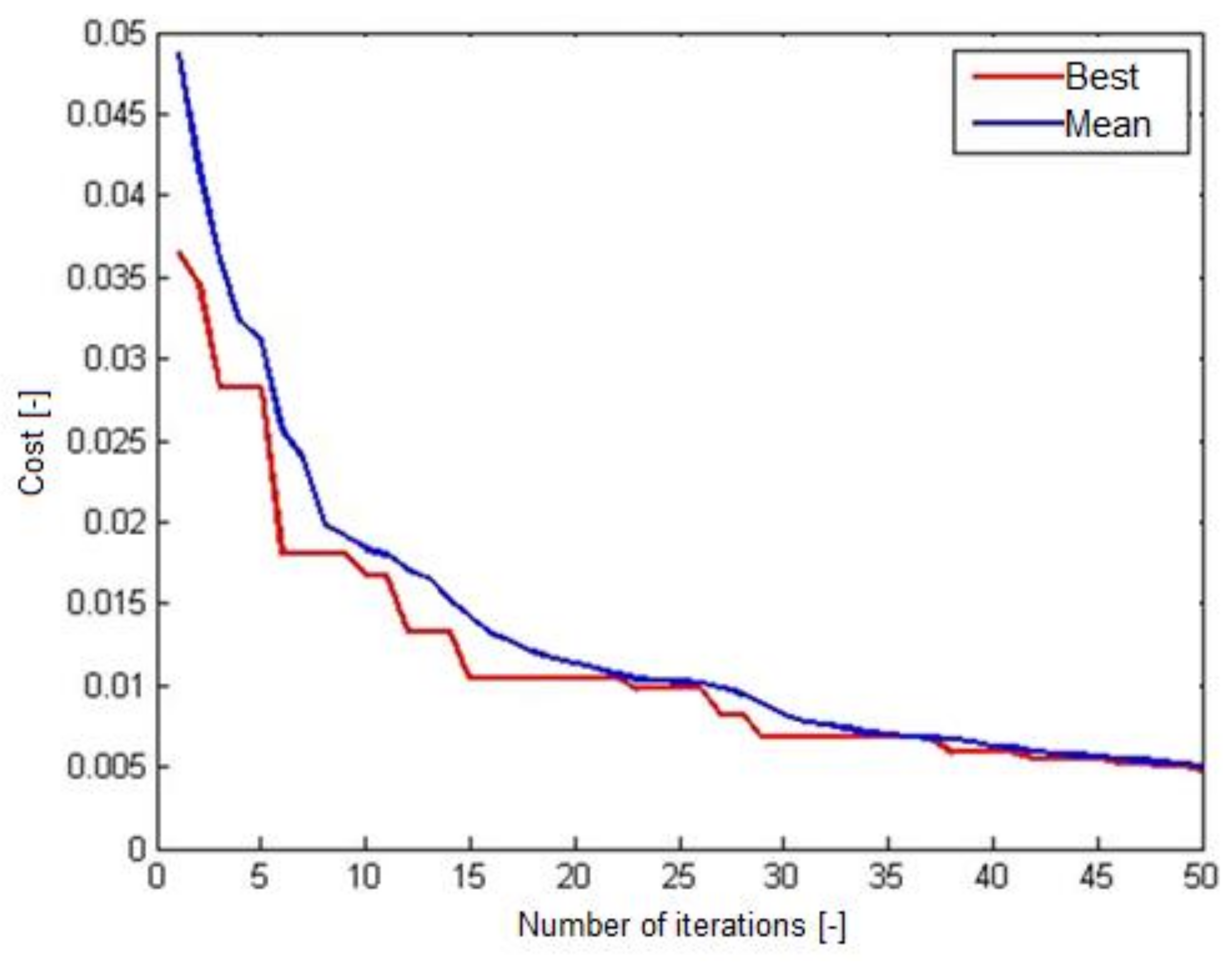
3.1. Selection of the Optimum Structure of the ANN Model
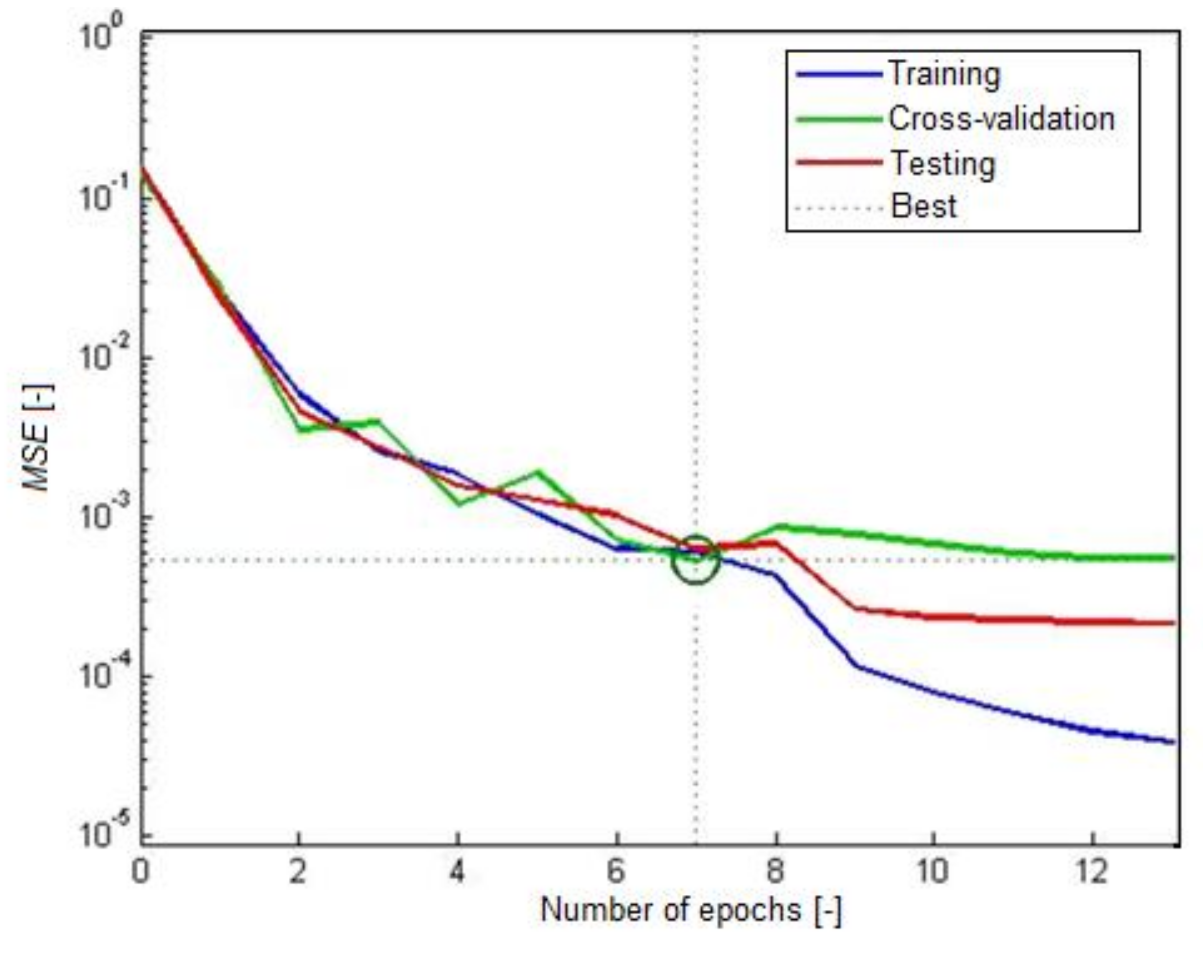
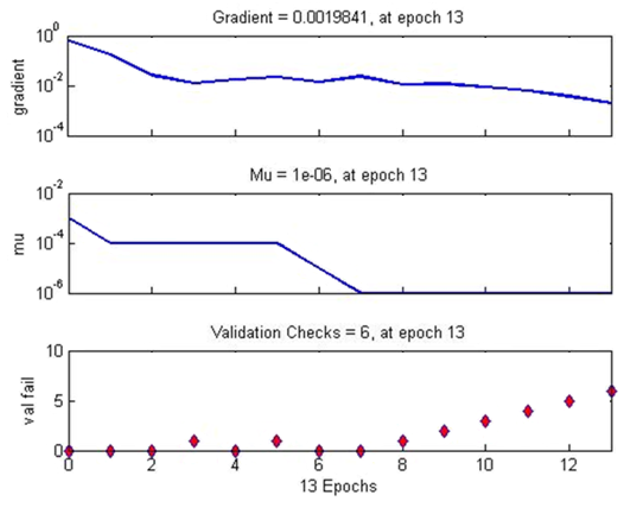
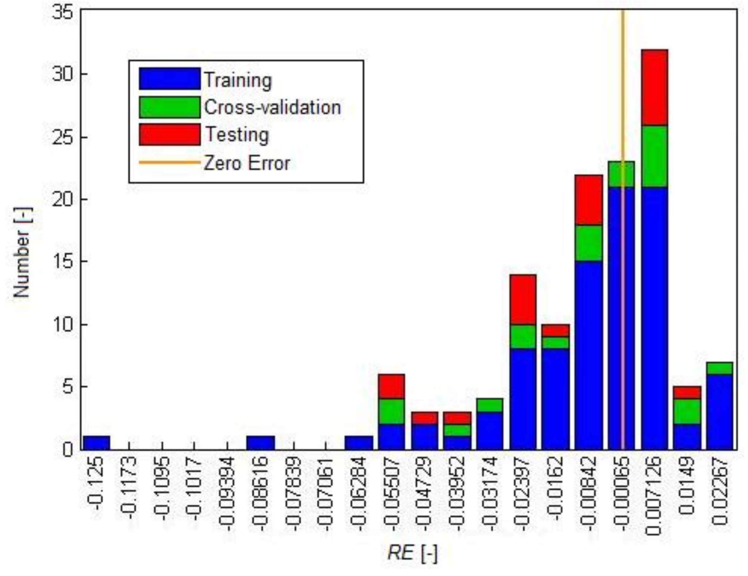
3.2. Results of Learning, Testing and Cross-Validation of the FA-ANN
3.3. Validation of the FA-ANN Model
4. Conclusions
- It is possible to predict the creep strain of green concrete with GGBFS using artificial neural networks (ANN) and the nature-inspired metaheuristic firefly algorithm (FA).
- A reliable prediction can be conducted based on the parameters of GGBFS concrete, which characterize the composition of the concrete mixture and selected rheological properties. For this purpose, the cement content, GGBFS content, water-to-binder ratio, fine aggregate content, coarse aggregate content, slump, the compaction factor of concrete and the age after loading were used as the input parameters, and in turn the creep strain (εcr) of GGBFS concrete was considered as the output parameter.
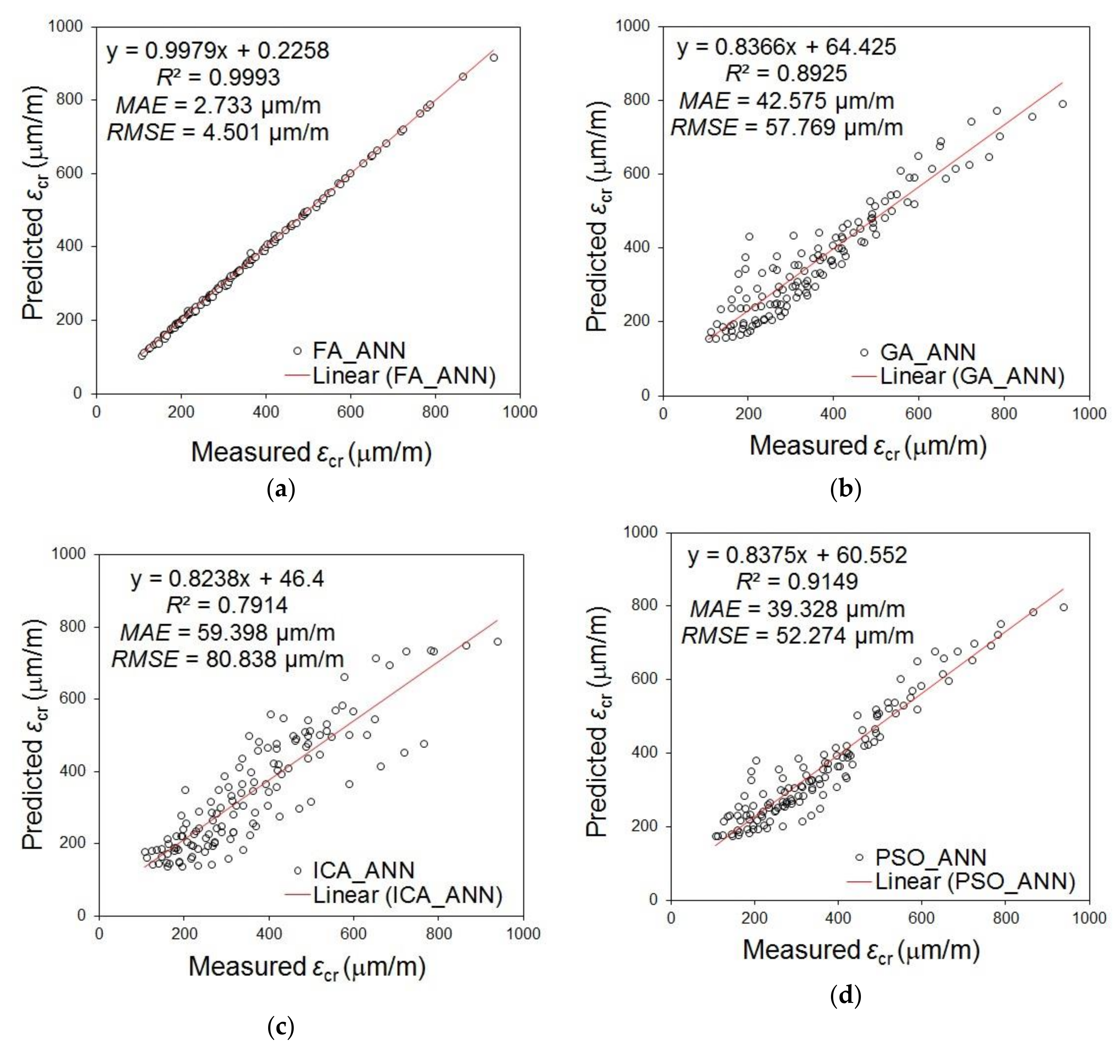
- The ANN model optimized by the FA was able to predict the value of εcr with a very high level of accuracy. The obtained values of determination coefficient (R2) were equal to 0.99 in training, cross-validation and testing.
- The performance of the FA-ANN was compared with other commonly used algorithms such as the imperialist competitive algorithm (ICA), genetic algorithm (GA) and particle swarm optimization (PSO). The obtained results indicated that the ANN model optimized by the FA was more accurate and provided more precision than other models.
Author Contributions
Funding
Conflicts of Interest
References
- El-Shafie, A.; Aminah, S. Dynamic versus static artificial neural network model for masonry creep deformation. Proc. Inst. Civ. Eng.-Struct. Build. 2013, 166, 355–366. [Google Scholar] [CrossRef]
- Hołowaty, J. Creep and Shrinkage of Concrete in Eurocode 2 and Polish Bridge Standards—Necessity for Implementation. J. Civ. Eng. Arch. 2015, 9, 460–466. [Google Scholar] [CrossRef]
- Özbay, E.; Erdemir, M.; Durmuş, H.İ. Utilization and efficiency of ground granulated blast furnace slag on concrete properties—A review. Constr. Build. Mater. 2016, 105, 423–434. [Google Scholar] [CrossRef]
- Barnett, S.J.; Soutsos, M.N.; Millard, S.G.; Bungey, J.H. Strength development of mortars containing ground granulated blast-furnace slag: Effect of curing temperature and determination of apparent activation energies. Cem. Concr. Res. 2006, 36, 434–440. [Google Scholar] [CrossRef]
- Young, C.H.; Chern, J.C. Practical prediction model for shrinkage of steel fibre reinforced concrete. Mater. Struct. 1991, 24, 191–201. [Google Scholar] [CrossRef]
- Han, M.Y.; Lytton, R.L. Theoretical prediction of drying shrinkage of concrete. ASCEJ. Mater. Civ. Eng. 1995, 7, 204–207. [Google Scholar] [CrossRef]
- Kim, J.K.; Lee, C.S. Prediction of differential drying shrinkage in concrete. Cem. Concr. Res. 1998, 28, 985–998. [Google Scholar] [CrossRef]
- Bazant, Z.P. Prediction of concrete creep and shrinkage: Past, present and future. Nucl. Eng. Des. 2001, 203, 27–38. [Google Scholar] [CrossRef]
- Eguchi, K.; Teranishi, K. Prediction equation of drying shrinkage of concrete based on composite model. Cem. Concr. Res. 2005, 35, 483–493. [Google Scholar] [CrossRef]
- Gardner, N.J. Design provisions for drying shrinkage and creep of normal strength concrete. ACI Mater. J. 2001, 98, 159–167. [Google Scholar]
- Shariq, M.; Prasad, J.; Abbas, H. Creep and drying shrinkage of concrete containing GGBFS. Cem. Concr. Compos. 2016, 68, 35–45. [Google Scholar] [CrossRef]
- Karthikeyan, J.; Upadhyay, A.; Bhandari, N.M. Artificial neural networks for predict creep and shrinkage of high performance concrete. J. Adv. Concr. Technol. 2008, 6, 135–142. [Google Scholar] [CrossRef]
- Gedam, B.A.; Bhandari, N.M.; Upadhyay, A. An apt material model for drying shrinkage and specific creep of HPC using artificial neural network. Struct. Eng. Mech. 2014, 52, 97–113. [Google Scholar] [CrossRef]
- Bal, L.; Bodin, F.B. Artificial neural network for predicting creep of concrete. Neural Comput. Appl. 2014, 25, 1359–1367. [Google Scholar] [CrossRef]
- Freidriks, A. Prediction models of shrinkage and creep in industrial floors and overlays, Degree Project. In Division of Concrete Structures; Second Level; KTH Royal Institute of Technology: Stockholm, Sweden, 2015. [Google Scholar]
- Asteris, P.G.; Roussis, P.C.; Douvika, M.G. Feed-Forward Neural Network Prediction of the Mechanical Properties of Sandcrete Materials. Sensors 2017, 17, 1344. [Google Scholar] [CrossRef] [PubMed]
- Cheng, M.Y.; Hoang, N.D. A self-adaptive fuzzy inference model based on least squares SVM for estimating compressive strength of rubberized concrete. Int. J. Inf. Technol. Decis. Mak. 2016, 15, 603–619. [Google Scholar] [CrossRef]
- Khademi, F.; Akbari, M.; Jamal, S.M.; Nikoo, M. Multiple linear regression, artificial neural network, and fuzzy logic prediction of 28 days compressive strength of concrete. Front. Struct. Civ. Eng. 2017, 11, 90–99. [Google Scholar] [CrossRef]
- Khademi, F.; Akbari, M.; Nikoo, M. Displacement Determination of Concrete Reinforcement Building using Data-Driven models. Int. J. Sustain. Built Environ. 2017, 6, 400–411. [Google Scholar] [CrossRef]
- Golafshani, E.M.; Behnood, A. Application of soft computing methods for predicting the elastic modulus of recycled aggregate concrete. J. Clean. Prod. 2018, 176, 1163–1176. [Google Scholar] [CrossRef]
- Golafshani, E.M.; Behnood, A. Automatic regression methods for formulation of elastic modulus of recycled aggregate concrete. Appl. Soft Comput. 2018, 64, 377–400. [Google Scholar] [CrossRef]
- Erzin, Y.; Nikoo, M.; Nikoo, M.; Cetin, T. The use of self-organizing feature map networks for the prediction of the critical factor of safety of an artificial slope. Neural Netw. World 2016, 26, 461–476. [Google Scholar] [CrossRef]
- Gandomi, A.H.; Sajedi, S.; Kiani, B.; Huang, Q. Genetic programming for experimental big data mining: A case study on concrete creep formulation. Autom. Construct. 2016, 70, 89–97. [Google Scholar] [CrossRef] [Green Version]
- IztokFister, I.F., Jr.; Yang, X.-S.; Brest, J. A comprehensive review of firefly algorithms. Swarm Evolut. Comput. 2013, 13, 34–46. [Google Scholar] [CrossRef] [Green Version]
- Yang, X.-S. Firefly Algorithm. In Engineering Optimization; John Wiley: Hoboken, NJ, USA, 2010; Volume 17. [Google Scholar]
- Bui, D.K.; Nguyen, T.; Chou, J.S.; Nguyen-Xuan, H.; Ngo, T.D. A modified firefly algorithm-artificial neural network expert system for predicting compressive and tensile strength of high-performance concrete. Construct. Build. Mater. 2018, 180, 320–333. [Google Scholar] [CrossRef]
- Sheikholeslami, R.; Khalili, B.G.; Sadollah, A.; Kim, J. Optimization of reinforced concrete retaining walls via hybrid firefly algorithm with upper bound strategy. KSCE J. Civ. Eng. 2016, 20, 2428–2438. [Google Scholar] [CrossRef]
- Nigdeli, S.M.; Bekdaş, G.; Yang, X.S. Metaheuristic optimization of reinforced concrete footings. KSCE J. Civ. Eng. 2018, 22, 1–9. [Google Scholar] [CrossRef]
- IS 8112. 43 Grade Ordinary Portland Cement—Specification; Bureau of Indian Standards: New Delhi, India, 1989. [Google Scholar]
- IS 12089. Indian Standard Specification for Granulated Slag for Manufacture of Portland Slag Cement; Bureau of Indian Standards: New Delhi, India, 1999. [Google Scholar]
- Shariq, M. Studies in Creep Characteristics of Concrete and Reinforced Concrete. Ph.D. Thesis, IIT Roorkee, Roorkee, India, 2008. [Google Scholar]
- IS 516. Indian standard: Methods of Tests for Strength of Concrete; Bureau of Indian Standards: New Delhi, India, 1999. [Google Scholar]
- Shariq, M.; Prasad, J.; Masood, A. Effect of GGBFS on time dependent compressive strength of concrete. Construct. Build. Mater. 2010, 24, 1469–1478. [Google Scholar] [CrossRef]
- Shapiro, S.; Wilk, M. An analysis of variance test for normality. Biometrika 1965, 52, 591–611. [Google Scholar] [CrossRef]
- Snedecor, G.W. Calculation and Interpretation of Analysis of Variance and Covariance; Collegiate Press, Inc.: Ames, Iowa, 1934. [Google Scholar]
- Bažant, Z.P.; Jirásek, M. Creep and Hygrothermal Effects in Concrete Structures; Springer: Berlin, Germany, 2018; Volume 225. [Google Scholar]
- Hecht-Nielson, R. Kolmogorov’s mapping neural network existence theorem. In Proceedings of the First IEEE International Joing Conference on Neural Networks, San Diego, CA, USA, 13–17 July 1987. [Google Scholar]
- Rogers, L.L.; Dowla, F.U. Optimization of groundwater remediation using artificial neural networks with parallel solute transport modeling. Water Resour. Res. 1994, 30, 457–481. [Google Scholar]


| Characteristic | Experimental Value | |
|---|---|---|
| Cement | GGBFS | |
| Blaine’s fineness (m2/kg) | 245 | 340 |
| Specific gravity | 3.15 | 2.86 |
| Soundness (mm) | 1.5 | 1.5 |
| Compressive strength (MPa) | 45.9 | 40 (with 30% GGBFS) |
| Normal Consistency (%) OPC + 0% GGBFS OPC + 20% GGBFS OPC + 40% GGBFS OPC + 60% GGBFS | 27.0 28.5 29.5 31.0 | |
| Name of Oxide | Cement (%) | GGBFS |
|---|---|---|
| CaO SiO2 Al2O3 Fe2O3 MgO Na2O K2O P2O5 TiO2 MnO Glass content | 63.71 22.18 07.35 03.82 0.95 0.28 0.11 0.05 0.27 0.04 - | 38.01 37.88 14.23 0.38 9.1 0.26 0.15 0.01 0.34 0.07 91.0 |
| Mix Group | Mix Designation | Cement | GGBFS | Aggregates (kg/m3) | Water-Binder Ratio | |
|---|---|---|---|---|---|---|
| (kg/m3) | (kg/m3) | Fine | Coarse | |||
| M1 | M10 M11 M12 M13 | 400 320 240 160 | 0 80 160 240 | 665 | 1107 | 0.45 |
| M2 | M20 M21 M22 M23 | 350 280 210 140 | 0 70 140 210 | 680 | 1132 | 0.50 |
| M3 | M30 M31 M32 M33 | 320 256 192 128 | 0 64 128 192 | 688 | 1145 | 0.55 |
| No. | Age t (days) | Cement Content C(kg/m3) | GGBFS Content G(kg/m3) | Water-to-Binder Ratio w/b (-) | Fine Aggregate Content Fa (kg/m3) | Coarse Aggregate Content Ca (kg/m3) | Slump S(mm) | Compaction Factor CF (-) | Creep Strain |
|---|---|---|---|---|---|---|---|---|---|
| 1 | 0 | 400 | 0 | 0.45 | 665 | 1107 | 41 | 0.9 | 106 |
| 2 | 1 | 400 | 0 | 0.45 | 665 | 1107 | 41 | 0.9 | 123 |
| 3 | 3 | 400 | 0 | 0.45 | 665 | 1107 | 41 | 0.9 | 145 |
| 4 | 7 | 400 | 0 | 0.45 | 665 | 1107 | 41 | 0.9 | 162 |
| 5 | 14 | 400 | 0 | 0.45 | 665 | 1107 | 41 | 0.9 | 181 |
| 6 | 21 | 400 | 0 | 0.45 | 665 | 1107 | 41 | 0.9 | 196 |
| 7 | 28 | 400 | 0 | 0.45 | 665 | 1107 | 41 | 0.9 | 204 |
| 8 | 56 | 400 | 0 | 0.45 | 665 | 1107 | 41 | 0.9 | 235 |
| 9 | 90 | 400 | 0 | 0.45 | 665 | 1107 | 41 | 0.9 | 261 |
| … | … | … | … | … | … | … | … | … | … |
| 132 | 150 | 128 | 192 | 0.55 | 688 | 1145 | 61 | 0.96 | 937 |
| Symbol and Name of Parameter | Statistical Characteristics | Shapiro–Wilk Test Results W | |||
|---|---|---|---|---|---|
| Mean | Minimum | Maximum | Standard Deviation | ||
| t - age after loading (days) | 44.54 | 0.00 | 150.00 | 50.26 | 0.796 |
| C - cement content (kg/m3) | 249.67 | 128.00 | 400.00 | 83.67 | 0.905 |
| G – GGBFS content (kg/m3) | 107.00 | 0.00 | 240.00 | 80.70 | 0.793 |
| w/b – water-to-binder ratio (-) | 0.50 | 0.45 | 0.55 | 0.04 | 0.769 |
| Fa - fine aggregate content (kg/m3) | 677.67 | 665.00 | 688.00 | 9.53 | 0.767 |
| Ca - coarse aggregate content (kg/m3) | 1128.00 | 1107.00 | 1145.00 | 15.77 | 0.937 |
| S - slump (mm) | 50.33 | 41.00 | 61.00 | 5.78 | 0.834 |
| CF - compaction factor (-) | 0.92 | 0.90 | 0.96 | 0.02 | 0.935 |
| -creep strain (μm/m) | 358.98 | 106.00 | 937.00 | 172,55 | 0.937 |
| Symbol and Name of Parameter | ρs | τ | F |
|---|---|---|---|
| t - age after loading (days) | 0.597 | 0.453 | 66.34 |
| C - cement content (kg/m3) | 0.788 | 0.612 | 13.14 |
| G – GGBFS content (kg/m3) | −0.473 | −0.345 | 11.36 |
| w/b – water-to-binder ratio (-) | 0.282 | 0.199 | 27.17 |
| Fa - fine aggregate content (kg/m3) | 0.437 | 0.342 | 27.16 |
| Ca - coarse aggregate content (kg/m3) | 0.437 | 0.342 | 27.16 |
| S - slump (mm) | 0.437 | 0.342 | 27.25 |
| CF - compaction factor (-) | 0.543 | 0.405 | 26.67 |
| FA | GA | ICA | PSO | ||||
|---|---|---|---|---|---|---|---|
| Attraction coefficient | 0.5 | Population | 150 | Number of initial countries | 500 | Swarm size | 100 |
| Mutation coefficient | 0.9 | Mutation rate | 15 | Number of initial imperialists | 50 | ||
| Number of fireflies | 10 | Crossover rate | 50 | Assimilation angle coefficient(β) | 2 | Cognition coefficient | 2 |
| Radius reduction factor | 0.95 | Angle coefficient (γ) | 0.5 | Social coefficient | 2 | ||
| Generation | 50 | Generation | 50 | Generation | 50 | Generation | 50 |
© 2019 by the authors. Licensee MDPI, Basel, Switzerland. This article is an open access article distributed under the terms and conditions of the Creative Commons Attribution (CC BY) license (http://creativecommons.org/licenses/by/4.0/).
Share and Cite
Sadowski, Ł.; Nikoo, M.; Shariq, M.; Joker, E.; Czarnecki, S. The Nature-Inspired Metaheuristic Method for Predicting the Creep Strain of Green Concrete Containing Ground Granulated Blast Furnace Slag. Materials 2019, 12, 293. https://doi.org/10.3390/ma12020293
Sadowski Ł, Nikoo M, Shariq M, Joker E, Czarnecki S. The Nature-Inspired Metaheuristic Method for Predicting the Creep Strain of Green Concrete Containing Ground Granulated Blast Furnace Slag. Materials. 2019; 12(2):293. https://doi.org/10.3390/ma12020293
Chicago/Turabian StyleSadowski, Łukasz, Mehdi Nikoo, Mohd Shariq, Ebrahim Joker, and Sławomir Czarnecki. 2019. "The Nature-Inspired Metaheuristic Method for Predicting the Creep Strain of Green Concrete Containing Ground Granulated Blast Furnace Slag" Materials 12, no. 2: 293. https://doi.org/10.3390/ma12020293