Analysis Method for Laterally Loaded Pile Groups Using an Advanced Modeling of Reinforced Concrete Sections


Abstract
:1. Introduction
2. Proposed ‘BEM-Based’ Method
2.1. Key Features of the Proposed Method
- a)
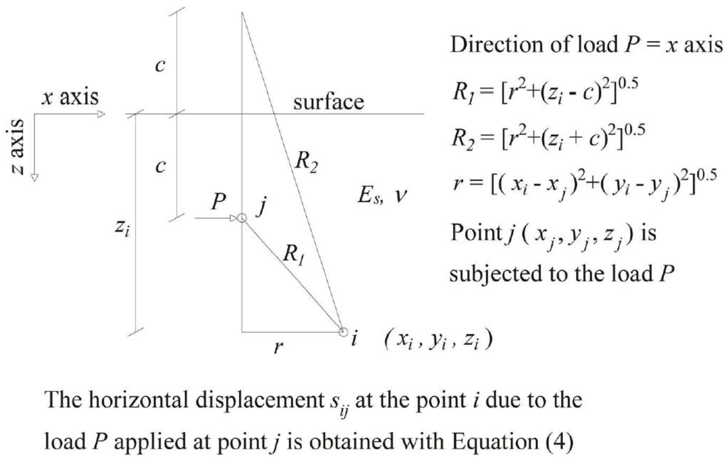
- pile-soil, pile-pile interactions are considered using the Mindlin’s solution;
- b)
- horizontally layered elastic soil;
- c)
- non-linear behavior for the reinforced concrete pile section;
- d)
- non-linear soil behavior (incremental analysis);
- e)
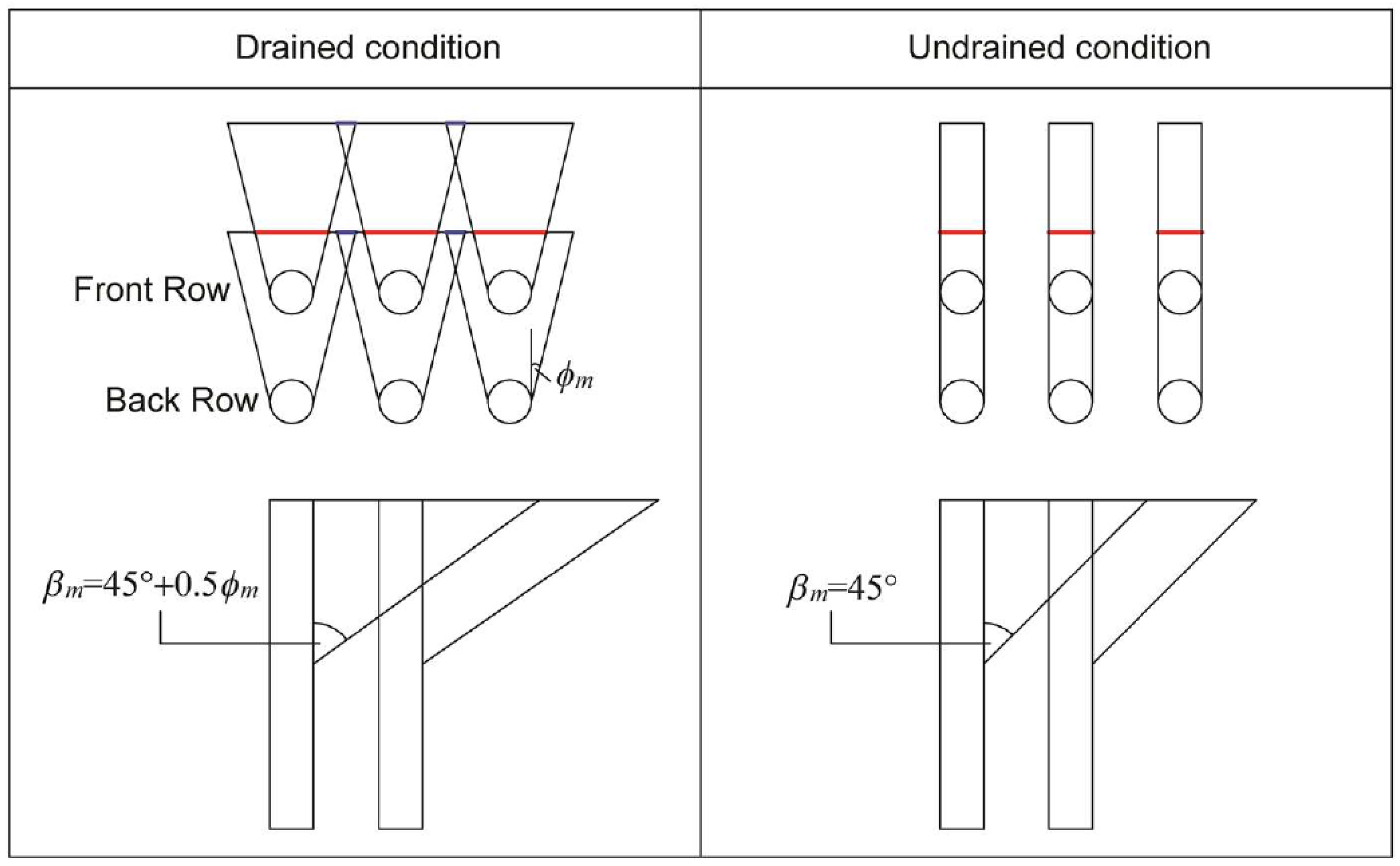
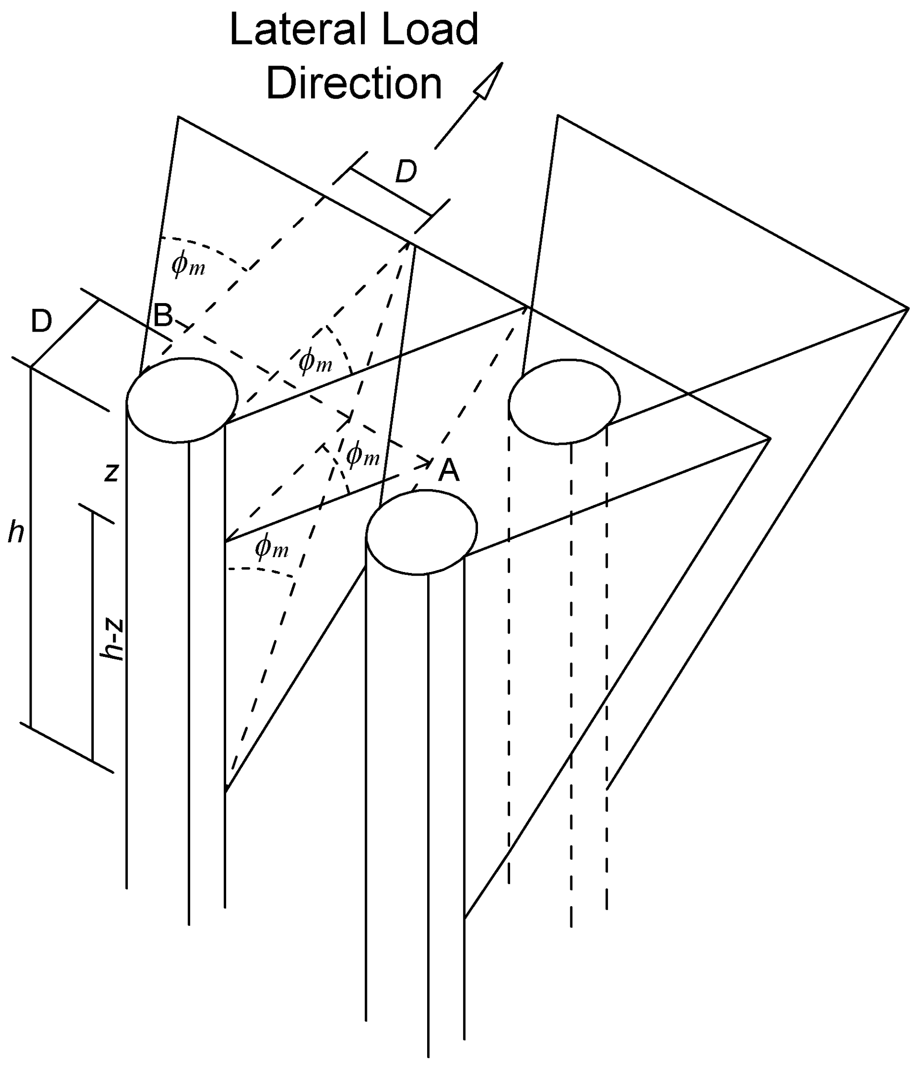
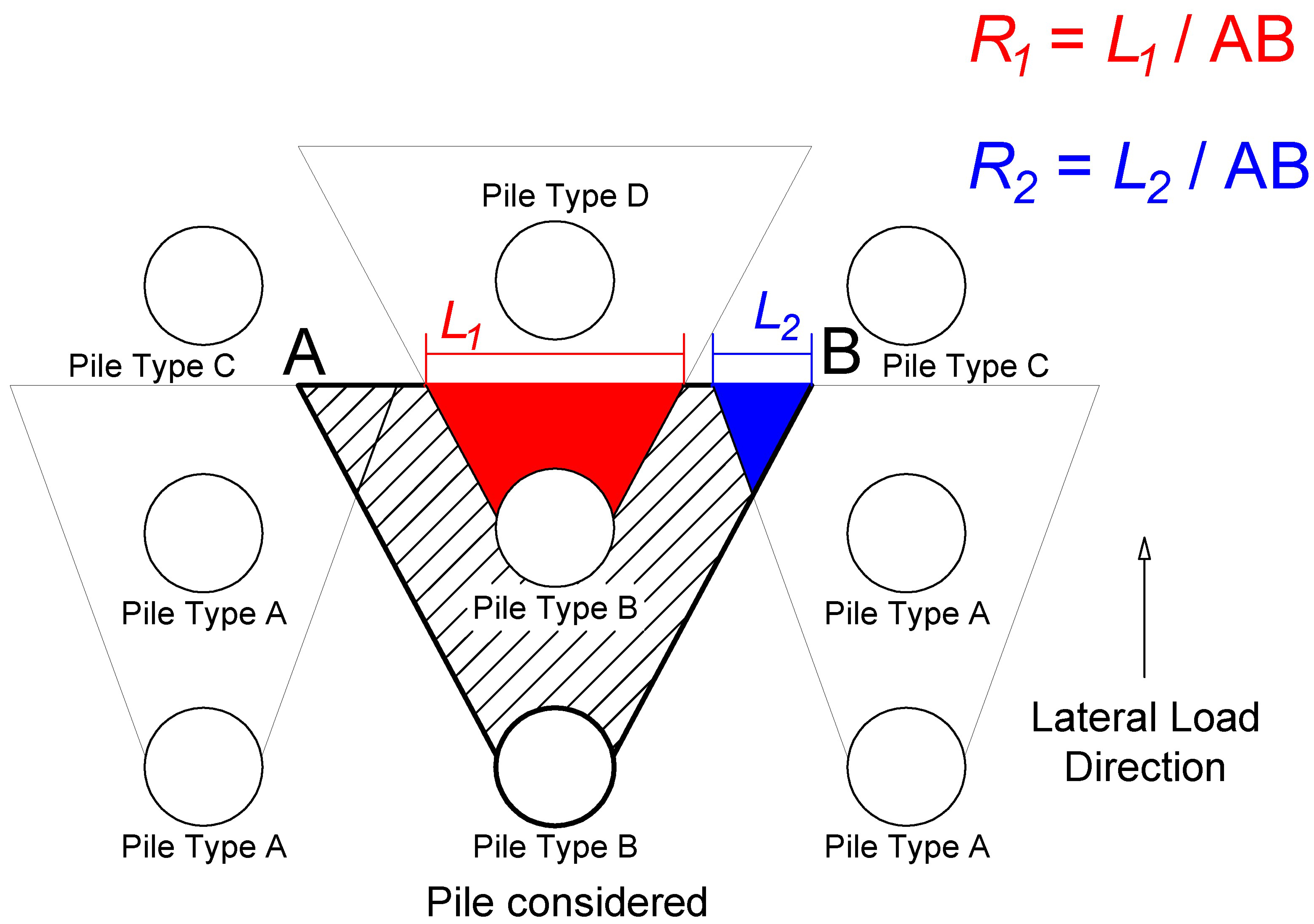
- the so-called shadowing effect, has been implemented in the code using an approach similar to that described in [35];
- f)
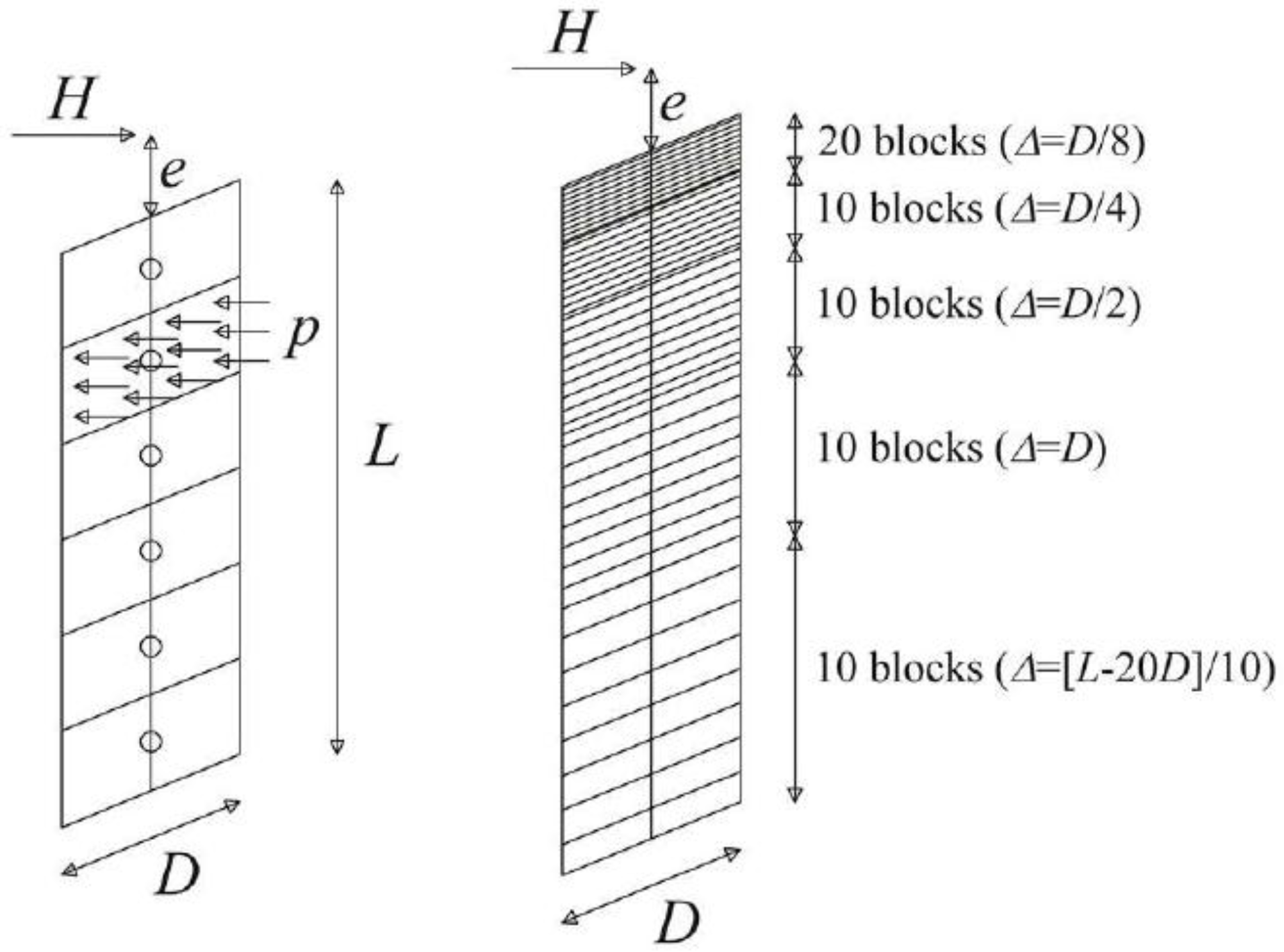
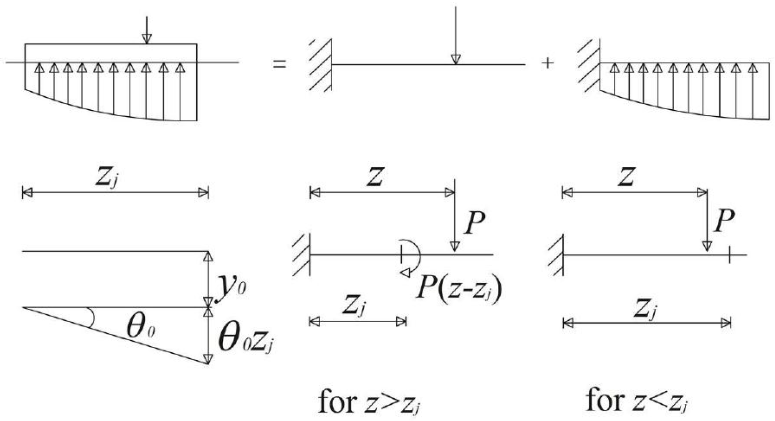
2.2. Pile Modelling
- 20 blocks with a thickness Δ = D/8, starting from the ground level up to a depth of 2.5D;
- 10 blocks with a thickness Δ = D/4, starting from a depth of 2.5D up to a depth of 5D;
- 10 blocks with a thickness Δ = D/2, starting from a depth of 5D up to a depth of 10D;
- 10 blocks with a thickness Δ = D, starting from a depth of 10D up to a depth of 20D;
- 10 blocks with a thickness Δ = (L − 20D)/10, starting from a depth of 20D up to the pile base depth.
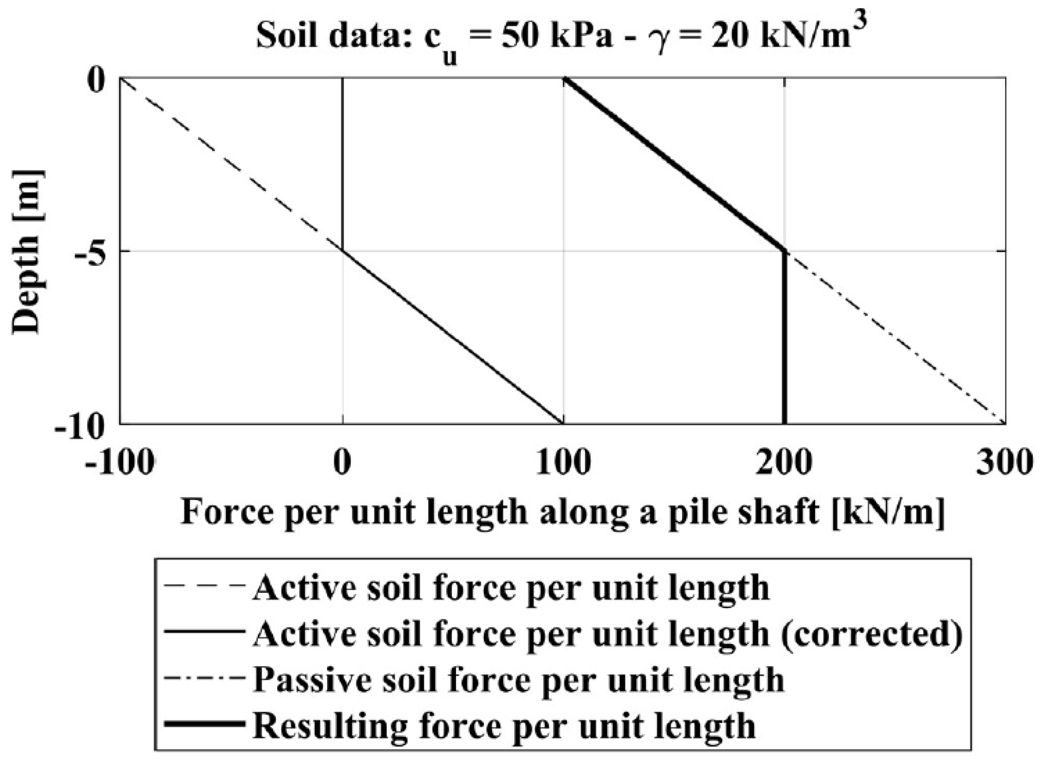
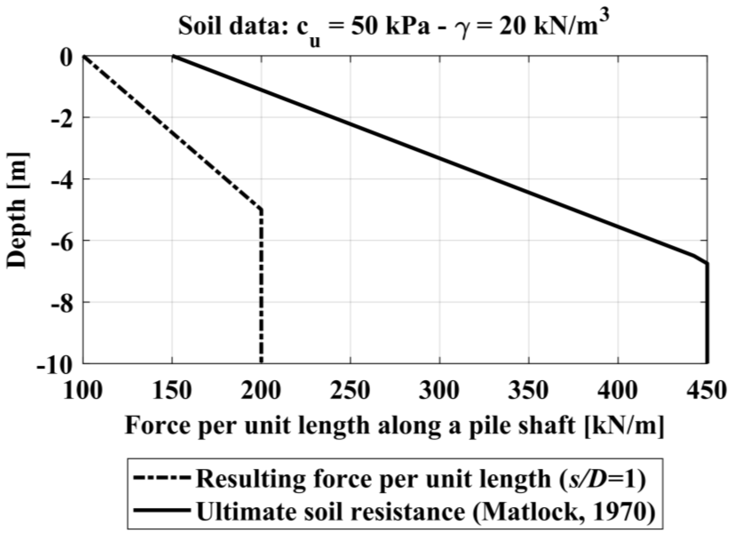
2.3. Soil Modelling
Soil Non-Linear Behavior
2.4. Influence of Suction on Pile Group Response to Horizontal Loading
2.5. Group Effects Modelling
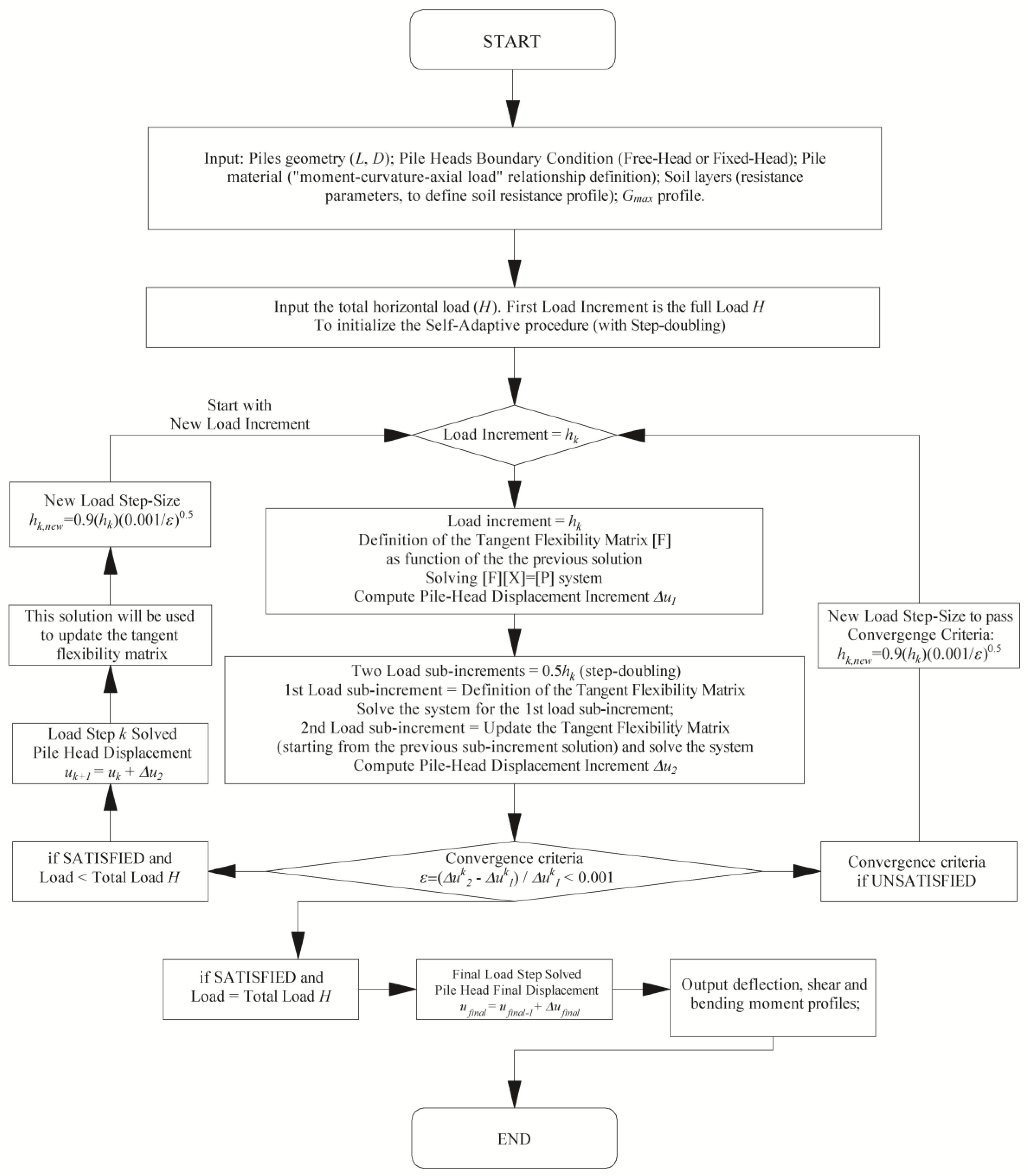
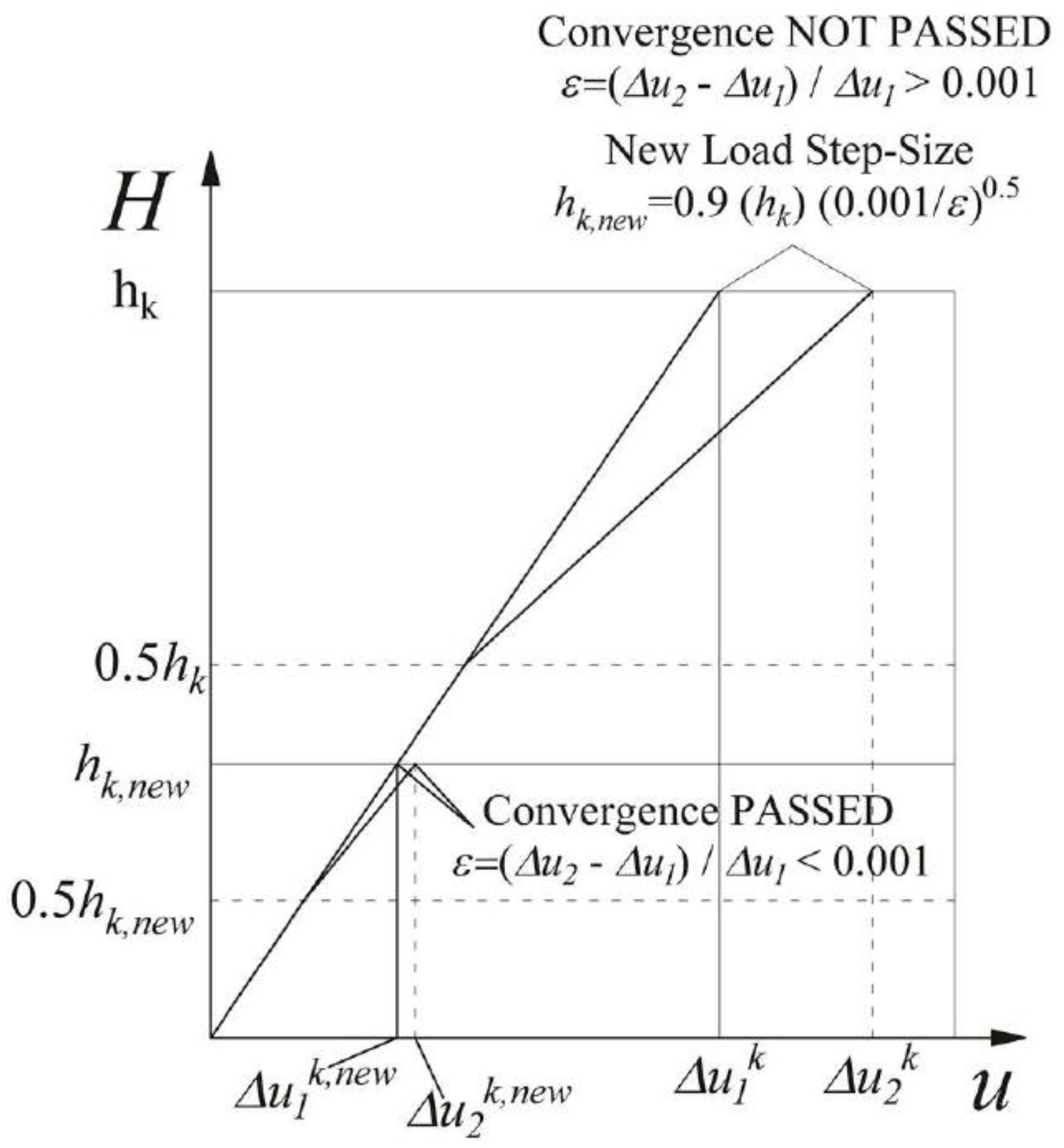
2.6. Solution System
- the km × km pile flexibility matrix [FP], composed of the aij coefficients;
- the km × km flexibility matrix [FS], composed of the bij coefficients that represent the displacements induced by a load acting at the pile-soil interface j to the pile-soil interface i.
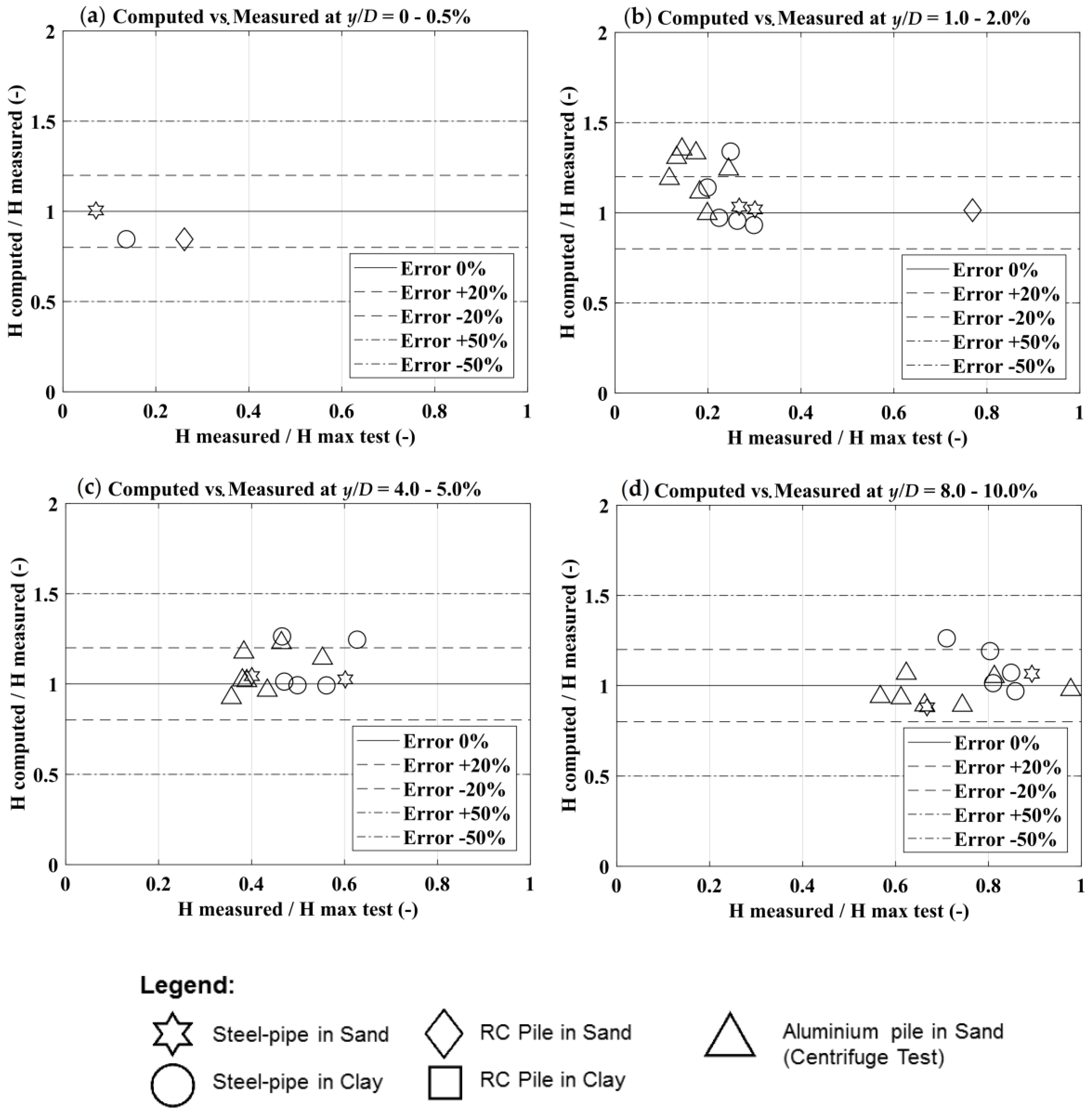
3. Validation of the Proposed Method
3.1. Analysis Results with the Proposed BEM Method for a Specific Lateral Load Test on a Bored Pile Group
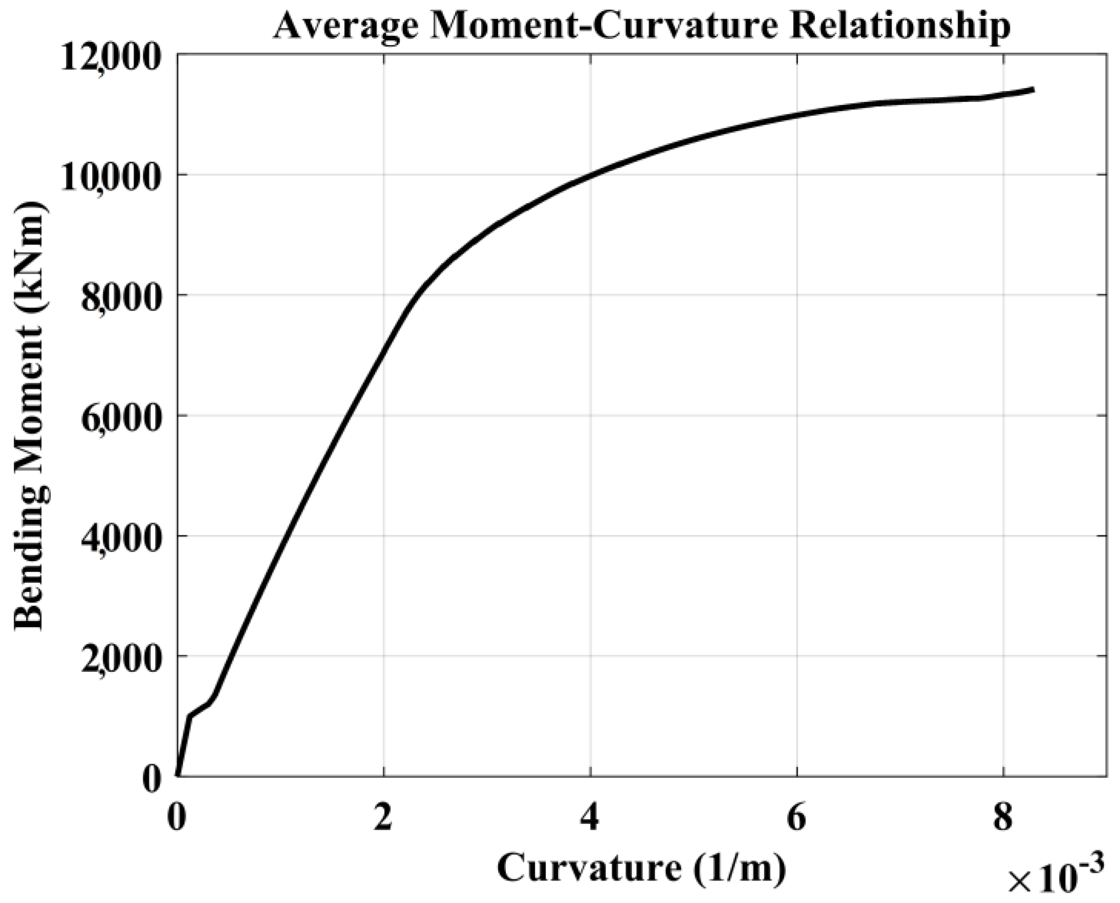
3.1.1. Soil and Pile Properties Description
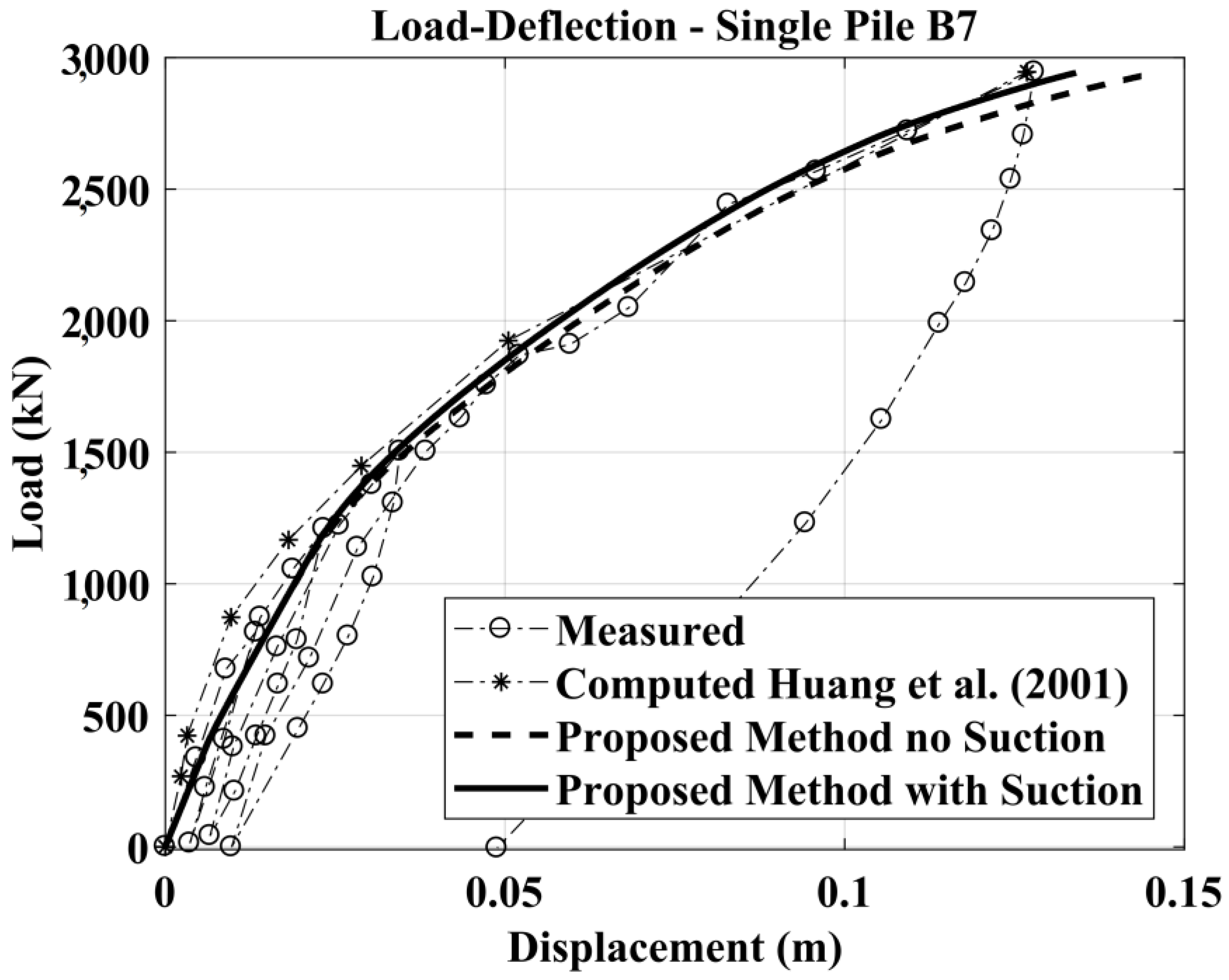
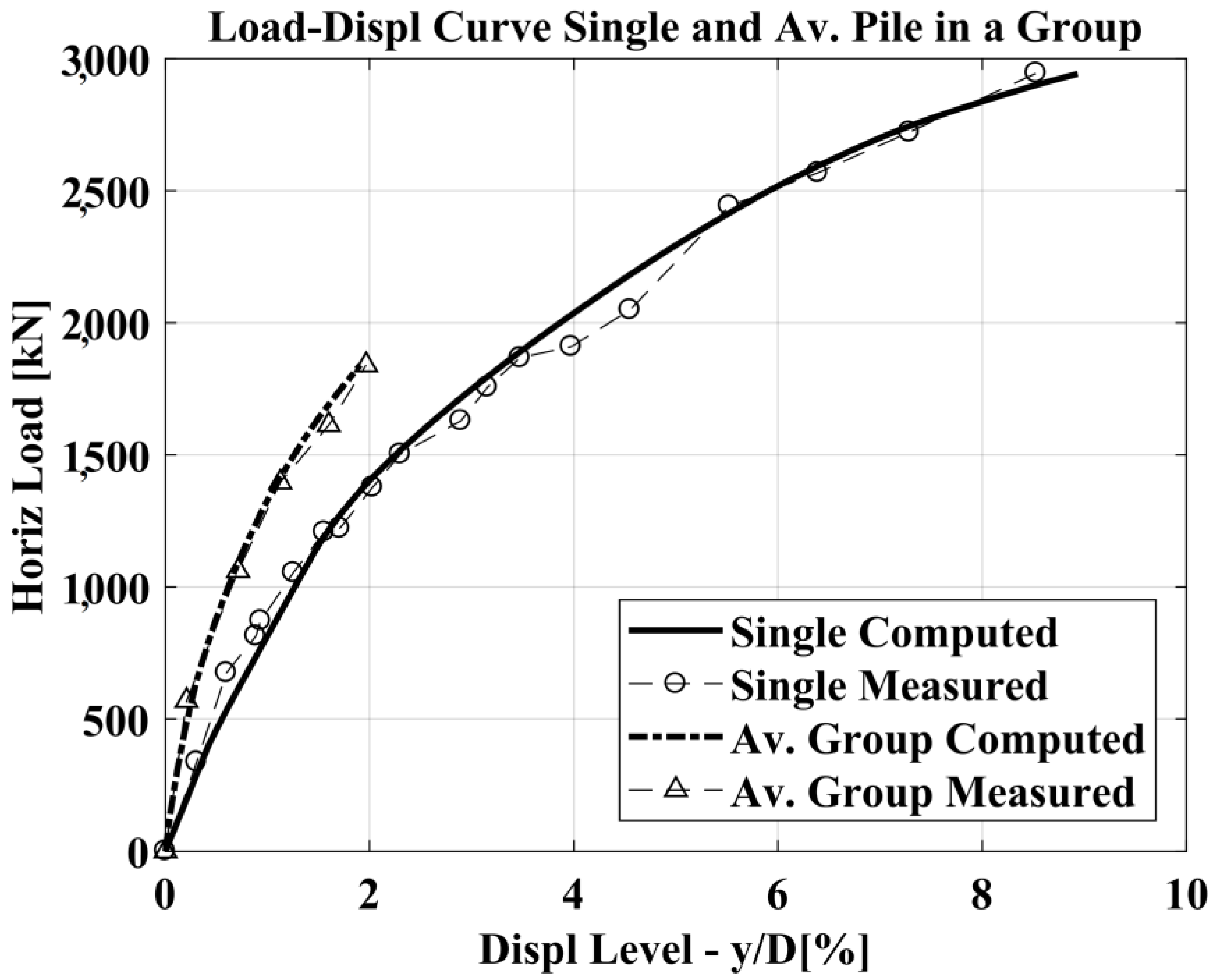
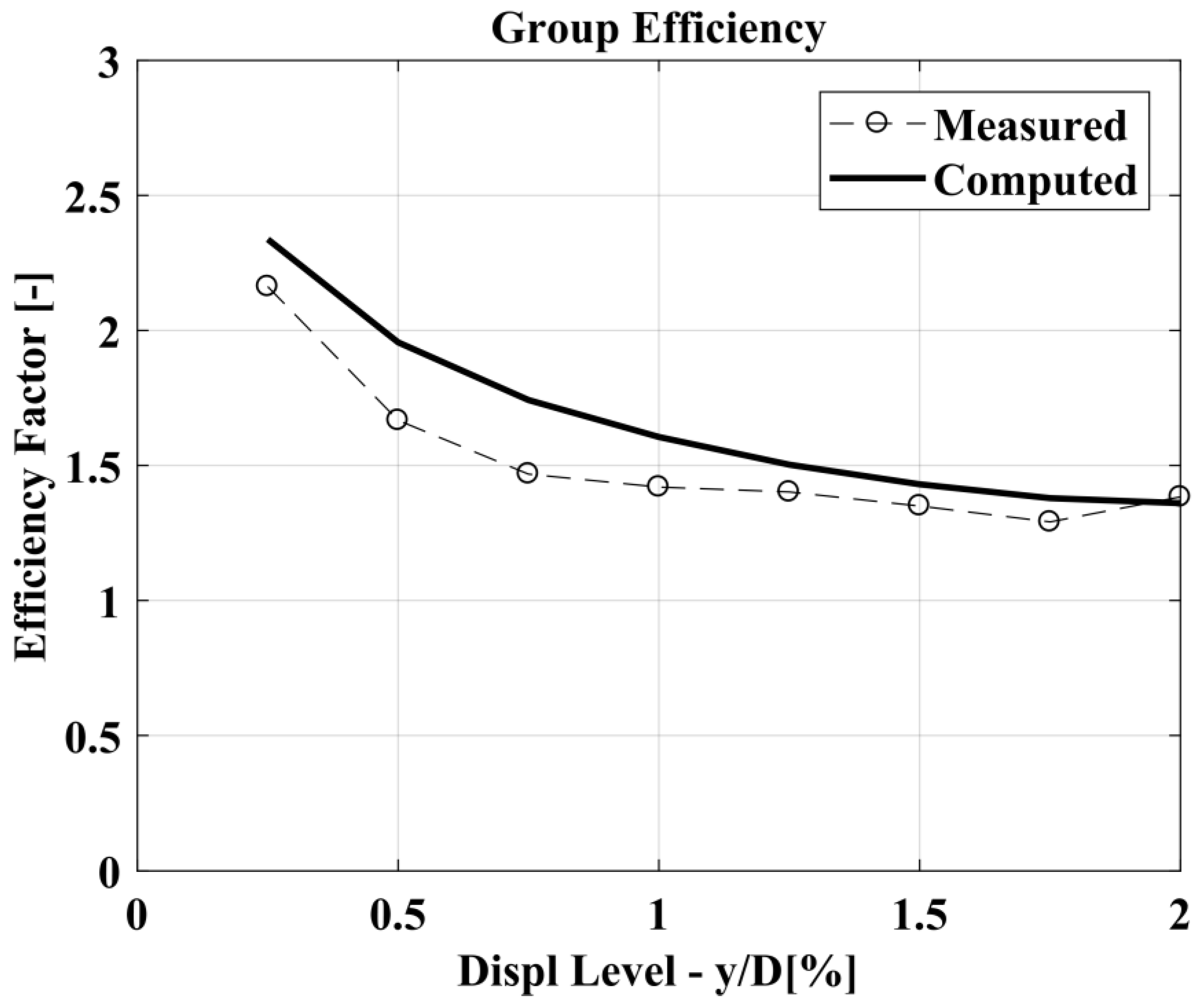
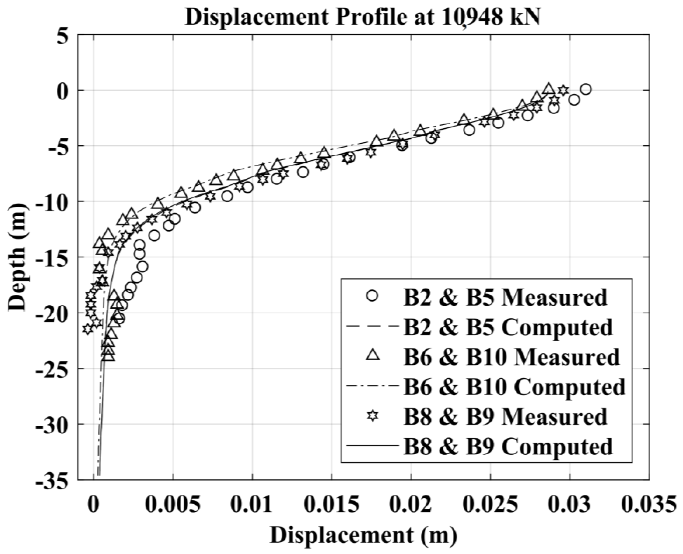
3.1.2. Single Bored Pile B7 (Free-Head) and Pile Group (Fixed-Head): Analysis Results
4. Conclusions
Acknowledgments
Author Contributions
Conflicts of Interest
References
- Mokwa, R.L.; Duncan, J.M. Experimental evaluation of lateral-load resistance of pile caps. J. Geotech. Geoenviron. Eng. 2001, 127, 185–192. [Google Scholar] [CrossRef]
- Katzenbach, R.; Turek, J. Combined pile-raft foundation subjected to lateral loads. In Proceedings of the International Conference on Soil Mechanics and Geotechnical Engineering, Osaka, Japan, 12–16 Spetember 2005; p. 2001. [Google Scholar]
- O’Neill, M.; Dunnavant, T.W. A Study of the Effects of Scale, Velocity, and Cyclic Degradability on Laterally Loaded Single Piles in Overconsolidated Clay; University of Houston: Houston, TX, USA, 1984. [Google Scholar]
- Huang, A.B.; Hsueh, C.K.; O’Neill, M.W.; Chern, S.; Chen, C. Effects of construction on laterally loaded pile groups. J. Geotech. Geoenviron. Eng. 2001, 127, 385–397. [Google Scholar] [CrossRef]
- Brown, D.; Morrison, C.; Reese, L. Lateral load behavior of pile group in sand. J. Geotech. Eng. 1988, 114, 1261–1276. [Google Scholar] [CrossRef]
- McVay, M.; Zhang, L.; Molnit, T.; Lai, P. Centrifuge Testing of Large laterally loaded Pile Groups in Sand. J. Geotech. Geoenviron. Eng. 1998, 124, 1016–1026. [Google Scholar] [CrossRef]
- Lateral-Load Tests on 25.4 mm (1-in.) Diameter Piles in Very Soft Clay in Side-by-Side and in-Line Groups; ASTM: West Conshohocken, PA, USA, 1984; STP 835; pp. 122–139.
- McVay, M.; Casper, R.; Shang, T.I. Lateral response of three-row groups in loose to dense sands at 3D and 5D pile spacing. J. Geotech. Eng. 1995, 121, 436–441. [Google Scholar] [CrossRef]
- Rollins, K.M.; Gerber, T.M.; Lane, J.D.; Ashford, S.A. Lateral resistance of a full-scale pile group in liquefied sand. J. Geotech. Geoenviron. Eng. 2005, 131, 115–125. [Google Scholar] [CrossRef]
- Mokwa, R. Investigation of the Resistance of Pile Caps to Lateral Loading. PhD Thesis, Virginia Polytechnic and State University, Blacksburg, VA, USA, February 2000. [Google Scholar]
- Rollins, K.; Lane, J.; Gerber, T. Measured and computed lateral response of a pile group in sand. J. Geotech. Geoenviron. Eng. 2006, 132, 103–114. [Google Scholar] [CrossRef]
- Reese, L.C.; Wang, S.T.; Isenhower, W.M.; Arrellaga, J.A. Computer Program Lpile Plus Version 5.0 Technical Manual; Ensoft: Austin, TX, USA, 2004. [Google Scholar]
- Reese, L.C.; Wang, S.T.; Arrellaga, J.A.; Hendrix, J. Computer Program GROUP for Windows, User’s Manual, Version 4.0; Ensoft: Austin, TX, USA, 1996. [Google Scholar]
- Hoit, M.I.; McVay, M.; Hays, C.; Andrade, P.W. Nonlinear pile foundation analysis using Florida-Pier. J. Bridg. Eng. 1996, 1, 135–142. [Google Scholar] [CrossRef]
- Abdrabbo, F.M.; Gaaver, K.E. Simplified analysis of laterally loaded pile groups. Alexandria Eng. J. 2012, 51, 121–127. [Google Scholar] [CrossRef]
- Hirai, H. A Winkler model approach for vertically and laterally loaded piles in nonhomogeneous soil. Int. J. Numer. Anal. Methods Geomech. 2012, 36, 1869–1897. [Google Scholar] [CrossRef]
- Khari, M.; Kassim, K.A.; Adnan, A. Development of Curves of Laterally Loaded Piles in Cohesionless Soil. Sci. World J. 2014, 2014, 917174. [Google Scholar] [CrossRef] [PubMed]
- Mardfekri, M.; Gardoni, P.; Roesset, J.M. Modeling laterally loaded single piles accounting for nonlinear soil-pile interactions. J. Eng. 2013, 2013, 243719. [Google Scholar] [CrossRef]
- Yang, Z.; Jeremić, B. Numerical analysis of pile behavior under lateral loads in layered elastic–plastic soils. Int. J. Numer. Anal. Methods Geomech. 2002, 26, 1385–1406. [Google Scholar] [CrossRef]
- Yang, Z.; Jeremić, B. Numerical study of group effects for pile groups in sands. Int. J. Numer. Anal. Methods Geomech. 2003, 27, 1255–1276. [Google Scholar] [CrossRef]
- Mindlin, R.D. Force at a point in the interior of a semi-infinite solid. Physics 1936, 7, 195–202. [Google Scholar] [CrossRef]
- Spillers, W.R.; Stoll, R.D. Lateral response of piles. J. Soil Mech. Found. Div. 1964, 90, 1–10. [Google Scholar]
- Poulos, H.G.; Davis, E.H. Pile Foundation Analysis and Design; Wiley & Sons: New York, NY, USA, 1980. [Google Scholar]
- Davies, T.G.; Banerjee, P.K. The displacement field due to a point load at the interface of a two layer elastic half-space. Geotechnique 1978, 28, 43–56. [Google Scholar] [CrossRef]
- Sharnouby, B.E.; Novak, M. Flexibility coefficients and interaction factors for pile group analysis. Can. Geotech. J. 1986, 23, 441–450. [Google Scholar] [CrossRef]
- Budhu, M.; Davies, T.G. Nonlinear analysis of laterality loaded piles in cohesionless soils. Can. Geotech. J. 1987, 24, 289–296. [Google Scholar] [CrossRef]
- Budhu, M.; Davies, T.G. Analysis of Laterally Loaded Piles in Soft Clays. J. Geotech. Eng. 1988, 114, 21–39. [Google Scholar] [CrossRef]
- Poulos, H.G. User’s Guide to Program DEFPIG 3/4 Deformation Analysis of Pile Groups; University of Sydney: Sydney, Australia, 1990. [Google Scholar]
- Randolph, M.F. PIGLET: A Computer Program for the Analysis and Design of Pile Groups; Report Geo 86033; University of Western Australia: Perth, Australia, 1987. [Google Scholar]
- Basile, F. A practical method for the non-linear analysis of piled rafts. In Proceedings of the 18th International Conference on Soil Mechanics and Geotechnical Engineering, Paris, France, 2–5 September 2013; p. 2503. [Google Scholar]
- Matos Filho, R.; Mendonça, A.V.; Paiva, J.B. Static boundary element analysis of piles submitted to horizontal and vertical loads. Eng. Anal. Bound. Elem. 2005, 29, 195–203. [Google Scholar] [CrossRef]
- Kitiyodom, P.; Matsumoto, T.; Horikoshi, K. Analyses of vertical and horizontal load tests on piled raft models in dry sand. In Proceedings of the International Conference on Soil Mechanics and Geotechnical Engineering, Osaka, Japan; 2005; pp. 2005–2008. [Google Scholar]
- Small, J.C.; Zhang, H.H. Piled raft foundations subjected to general loadings. In Proceedings of the Developments in Theoretical Geomechanics, Sydney, Australia, 1 January 2000; pp. 57–72. [Google Scholar]
- Ashour, M.; Norris, G.; Pilling, P. Lateral Loading of a Pile in Layered Soil Using the Strain Wedge Model. J. Geotech. Geoenviron. Eng. 1998, 124, 303–315. [Google Scholar] [CrossRef]
- Ashour, M.; Pilling, P.; Norris, G. Lateral Behavior of Pile Groups in Layered Soils. J. Geotech. Geoenviron. Eng. 2004, 130, 580–592. [Google Scholar] [CrossRef]
- Fahey, M.; Carter, J. A finite element study of the pressuremeter test in sand using a nonlinear elastic plastic model. Can. Geotech. J. 1993, 30, 348–362. [Google Scholar] [CrossRef]
- Matlock, H. Correlations for design of laterally loaded piles in soft clay. In Proceedings of the 2nd Annual Offshore Technology Conference, Houston, TX, USA, 22–24 April 1970; pp. 577–588. [Google Scholar]
- Reese, L.C.; Cox, W.R.; Koop, F.D. Analysis of laterally loaded piles in sand. In Proceedings of the VI Annual Offshore Technology Conference, Houston, TX, USA; 1974; pp. 473–485. [Google Scholar]
- Welch, R.C.; Reese, L.C. Lateral Load Behavior of Drilled Shafts; University of Texas: Austin, TX, USA, 1972. [Google Scholar]
- Reese, L.; Cox, W.; Koop, F. Field testing and analysis of laterally loaded piles in stiff clay. Proceedings of Offshore Technology Conference, Houston, TX, USA, 5–8 May 1975; pp. 671–690. [Google Scholar]
- Landi, G. Pali soggetti a carichi orizzontali: Indagini sperimentali ed analisi. PhD Thesis, University of Naples Federico II, Pisa, Italia, 26–28 June 2006. [Google Scholar]
- Stacul, S.; Squeglia, N.; Morelli, F. Laterally Loaded Single Pile Response Considering the Influence of Suction and Non-Linear Behaviour of Reinforced Concrete Sections. Appl. Sci. 2017, 7, 1310. [Google Scholar] [CrossRef]
- Morelli, F.; Amico, C.; Salvatore, W.; Squeglia, N.; Stacul, S. Influence of Tension Stiffening on the Flexural Stiffness of Reinforced Concrete Circular Sections. Materials 2017, 10, 201. [Google Scholar] [CrossRef]
- Salvatore, W.; Buratti, G.; Maffei, B.; Valentini, R. Dual-phase steel re-bars for high-ductile r.c. structures, Part 2: Rotational capacity of beams. Eng. Struct. 2007, 29, 3333–3341. [Google Scholar] [CrossRef]
- Kondner, R.L. Hyperbolic Stress-Strain Response: Cohesive Soils. J. Soil Mech. Found. Div. 1963, 89, 115–144. [Google Scholar]
- Duncan, J.M.; Chang, C.Y. Nonlinear Analysis of Stress and Strain in Soil. J. Soil Mech. Found. Div. 1970, 96, 1629–1653. [Google Scholar]
- Hardin, B.O.; Drnevich, V.P. Shear Modulus and Damping in Soils: Design Equations and Curves. Soil Mech. Found. Div. 1972, SM7, 667–692. [Google Scholar]
- Aubertin, M.; Mbonimpa, M.; Bussière, B.; Chapuis, R.P. A model to predict the water retention curve from basic geotechnical properties. Can. Geotech. J. 2003, 40, 1104–1122. [Google Scholar] [CrossRef]
- Press, W.H.; Teukolsky, S.A.; Vetterling, W.T.; Flannery, B.P. Numerical Recipes in C++. The Art of Scientific Computing, 2nd ed.; Cambridge University Press: Cambridge, UK, 2002; pp. 714–718. [Google Scholar]
- Stacul, S. Analysis of piles and piled raft foundation under horizontal load. PhD Thesis, University of Florence, Florence, Italy, 2018. [Google Scholar]
- Brown, D.; Reese, L.; O’Neill, M. Cyclic lateral loading of a large-scale pile group. J. Geotech. Eng. 1987, 113, 1326–1343. [Google Scholar] [CrossRef]
- Remaud, D.; Garnier, J.; Frank, R. Laterally loaded piles in dense sand: Group effects. In Proceedings of the International Conference Centrifuge, Tokyo, Japan, 23–25 September 1998; pp. 533–538. [Google Scholar]
- Rollins, K.M.; Peterson, K.T.; Weaver, T.J. Lateral load behavior of full-scale pile group in clay. J. Geotech. Geoenviron. Eng. 1998, 124, 468–478. [Google Scholar] [CrossRef]
- Rollins, K.M.; Olsen, K.G.; Jensen, D.H.; Garrett, B.H.; Olsen, R.J.; Egbert, J.J. Pile spacing effects on lateral pile group behavior: Analysis. J. Geotech. Geoenviron. Eng. 2006, 132, 1272–1283. [Google Scholar] [CrossRef]
- Mayne, P.W. In situ test calibrations for evaluating soil parameters. In Proceedings of the Second International Workshop on Characterisation and Engineering Properties of Natural Soils, Singapore, Singapore, 29 November–1 December 2006; Tan, T.S., Phoon, K.K., Hight, D.W., Leroueil, S., Eds.; CRC Press: Boca Raton, FL, USA; pp. 1601–1652. [Google Scholar]
- Wu, G.; Finn, W.L.; Dowling, J. Quasi-3D analysis: Validation by full 3D analysis and field tests on single piles and pile groups. Soil Dyn. Earthq. Eng. 2015, 78, 61–70. [Google Scholar] [CrossRef]
- Reese, L.C.; Wang, S.T. LPILE 4.0.; Ensoft Inc.: Austin, TX, USA, 1993. [Google Scholar]
- Wu, G. VERSAT-P3D: A Computer Program for Dynamic 3-Dimensional Finite Element Analysis of Single Piles and Pile Groups; Wutec Geotechnical International: Vancouver, BC, Canada, 2006. [Google Scholar]
- Fayyazi, M.S.; Taiebat, M.; Finn, W.L. Group reduction factors for analysis of laterally loaded pile groups. Can. Geotech. J. 2014, 51, 758–769. [Google Scholar] [CrossRef]


| Case Reference | Pile Material | Pile Diameter (m) | Pile Length (m) | Soil Type | Hmax (kN) |
|---|---|---|---|---|---|
| [51] 3 × 3; s = 3D | Steel with Grout-fill | 0.273 | 13.11 | OC Clay | 695 |
| [5] 3 × 3; s = 3D | Steel with Grout-fill | 0.273 | 13.11 | Sand | 808.5 |
| [4] 3 × 2; s = 3D | Bored RC | 1.5 | 34.9 | Silty Sand | 11043 |
| [8] ϕ’ = 34°; 3 × 3; s =3D | Aluminum | 0.43 | 13.3 | Sand | 761.2 |
| [8] ϕ’ = 39°; 3 × 3; s = 3D | Aluminum | 0.43 | 13.3 | Sand | 1508.2 |
| [8] ϕ’ = 34°; 3 × 3; s = 5D | Aluminum | 0.43 | 13.3 | Sand | 1110.5 |
| [8] ϕ’ = 39°; 3 × 3; s = 5D | Aluminum | 0.43 | 13.3 | Sand | 1424 |
| [52] 2 × 1; s = 2D | Aluminum | 0.72 | 12 | Sand | 1183 |
| [52] 2 × 1; s = 4D | Aluminum | 0.72 | 12 | Sand | 1220.1 |
| [52] 2 × 1; s = 6D | Aluminum | 0.72 | 12 | Sand | 1030.72 |
| [53] 3 × 3; s = 3D | Steel with Grout-fill | 0.305 | 8.7 | Clay | 927.05 |
| [11] 3 × 3; s = 3D | Steel pipe | 0.324 | 11.5 | Sand | 488.6 |
| [54] 3 × 3; s = 5.65D | Steel pipe | 0.324 | 11.9 | Clay | 1407 |
| [54] 3 × 4; s = 4.4D | Steel pipe | 0.324 | 11.9 | Clay | 1353.8 |
| [54] 3 × 5; s = 3.3D | Steel pipe | 0.324 | 11.9 | Clay | 1942.5 |
| Case | EpIp (MNm2) | γ (kN/m3) | ϕ (°) | DR (%) | cu (kPa) | Emax (Linear Increasing with Depth) (MPa) | G (-) | F (m) | W.T. (m) | Head B.C. |
|---|---|---|---|---|---|---|---|---|---|---|
| [51] | 16.0 | 19.0 | - | - | 58–145 (0–5.5 m) | 70–200 (0–5.5 m) | 0.25 | 0.305 | 0.0 | Free |
| [5] | 16.0 | 19.5 | 47 | 90 | - | 35–100 (0–2.0 m) | 1.0 | 0.305 | 0.0 | Free |
| [4] | variable | 18.5 | 34 | 50 | - | 40–400 (0–34.9 m) | 0.5 | 1.0 | 1.0 | Fixed |
| [8] | 72.1 | 14.51 | 34 | 33 | - | 60–300 (0–13.3 m) | 0.25 | 1.68 | - | Free |
| [8] | 72.1 | 15.18 | 39 | 55 | - | 50–260 (0–13.3 m) | 0.5 | 1.68 | - | Free |
| [52] | 514.0 | 16.3 | 40 | 89 | - | 40–200 (0–12.0 m) | 1.0 | 1.6 | - | Free |
| [53] | 26.91 | 19.0 | - | - | 50–75 (0–2.9 m) | 60–170 (0–8.7 m) | 0.25 | 0.4 | 0.0 | Free |
| [11] | 30.03 | 19.5 | 40 | 44 | - | 20–150 (0–11.5 m) | 0.25 | 0.86 | 0.0 | Free |
| [54] | 30.03 | 19.0 | - | - | 60 (0–1 m)120 (1.0–4.0 m) | 50–60 (0–4.0 m) | 0.25 | 0.48 | 1.0 | Free |
| Pile Diameter D (mm) | Pile Length (m) | Cross Sectional Area (cm2) | Concrete Compressive Strength f’c (MPa) | Reinforcement Yield Stress fy (MPa) | Steel Ratio ρs | Intact Flexural Rigidity EI (GNm2) |
|---|---|---|---|---|---|---|
| 1500 | 34.9 | 17672 | 27.5 | 471 | 0.025 | 6.86 |
© 2018 by the authors. Licensee MDPI, Basel, Switzerland. This article is an open access article distributed under the terms and conditions of the Creative Commons Attribution (CC BY) license (http://creativecommons.org/licenses/by/4.0/).
Share and Cite
Stacul, S.; Squeglia, N. Analysis Method for Laterally Loaded Pile Groups Using an Advanced Modeling of Reinforced Concrete Sections. Materials 2018, 11, 300. https://doi.org/10.3390/ma11020300
Stacul S, Squeglia N. Analysis Method for Laterally Loaded Pile Groups Using an Advanced Modeling of Reinforced Concrete Sections. Materials. 2018; 11(2):300. https://doi.org/10.3390/ma11020300
Chicago/Turabian StyleStacul, Stefano, and Nunziante Squeglia. 2018. "Analysis Method for Laterally Loaded Pile Groups Using an Advanced Modeling of Reinforced Concrete Sections" Materials 11, no. 2: 300. https://doi.org/10.3390/ma11020300
APA StyleStacul, S., & Squeglia, N. (2018). Analysis Method for Laterally Loaded Pile Groups Using an Advanced Modeling of Reinforced Concrete Sections. Materials, 11(2), 300. https://doi.org/10.3390/ma11020300