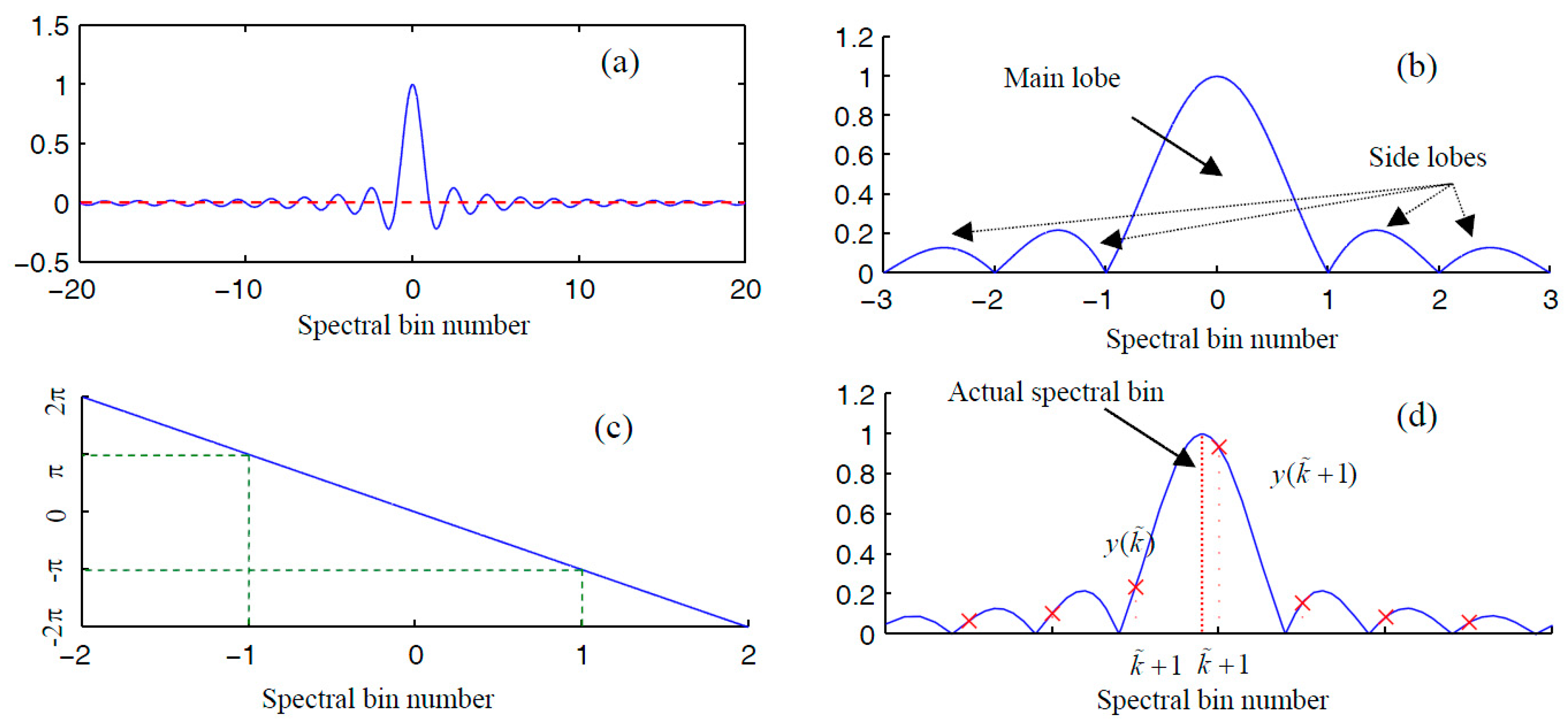
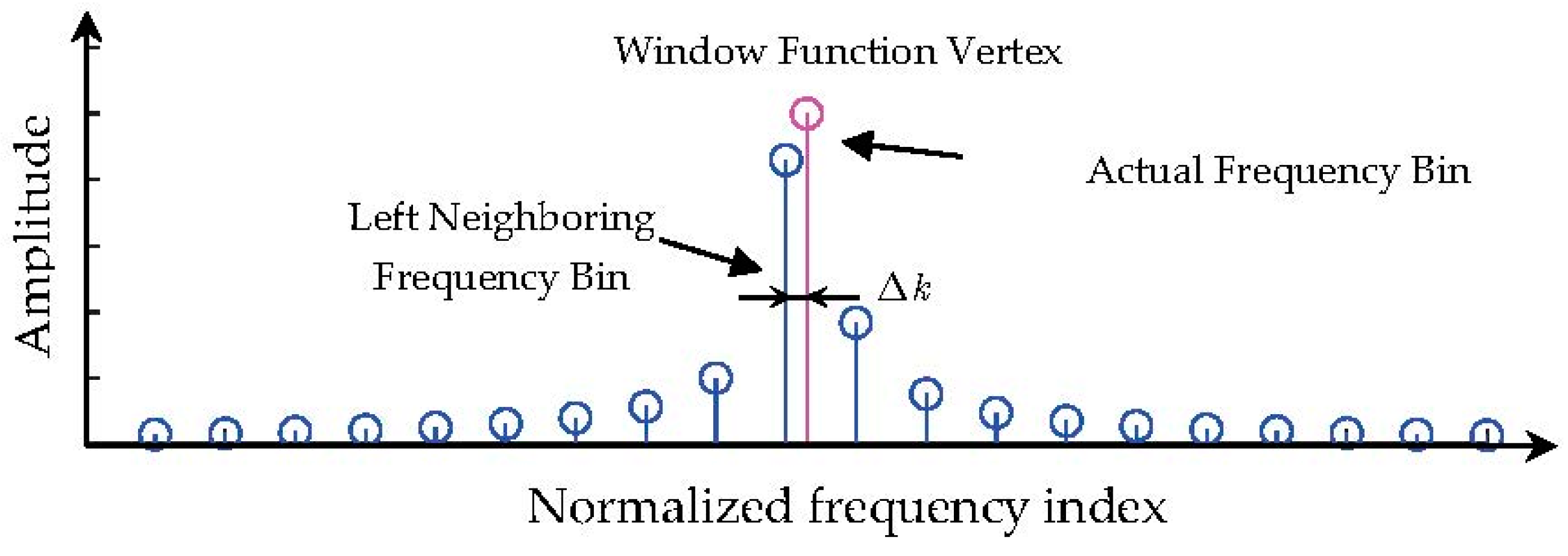
Figure 1.
Illustration of some notations of energy leakage problem in FFT.
Figure 1.
Illustration of some notations of energy leakage problem in FFT.
Figure 2.
Fundamental principles of a rectangular-window-based spectral correction method. (a) The magnitude response; (b) zoomed-in plot of the magnitude response; (c) the phase response; and (d) the FFT grids compared with the magnitude response.
Figure 2.
Fundamental principles of a rectangular-window-based spectral correction method. (a) The magnitude response; (b) zoomed-in plot of the magnitude response; (c) the phase response; and (d) the FFT grids compared with the magnitude response.
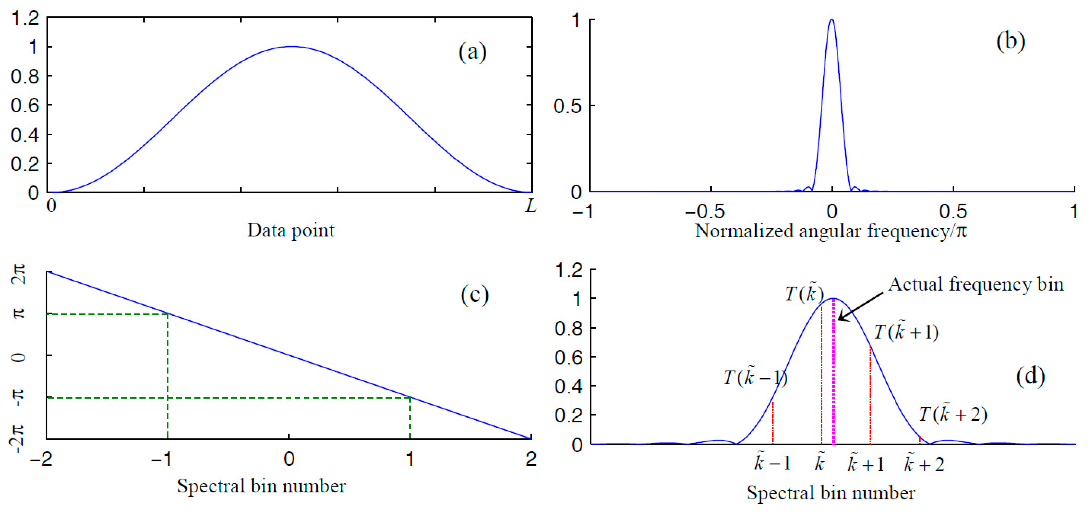
Figure 3.
Fundamental principles of Hanning-window-based spectral correction method. (a) The magnitude response; (b) a zoomed-in plot of the magnitude response; (c) the phase response; and (d) the FFT grids compared with the magnitude response.
Figure 3.
Fundamental principles of Hanning-window-based spectral correction method. (a) The magnitude response; (b) a zoomed-in plot of the magnitude response; (c) the phase response; and (d) the FFT grids compared with the magnitude response.
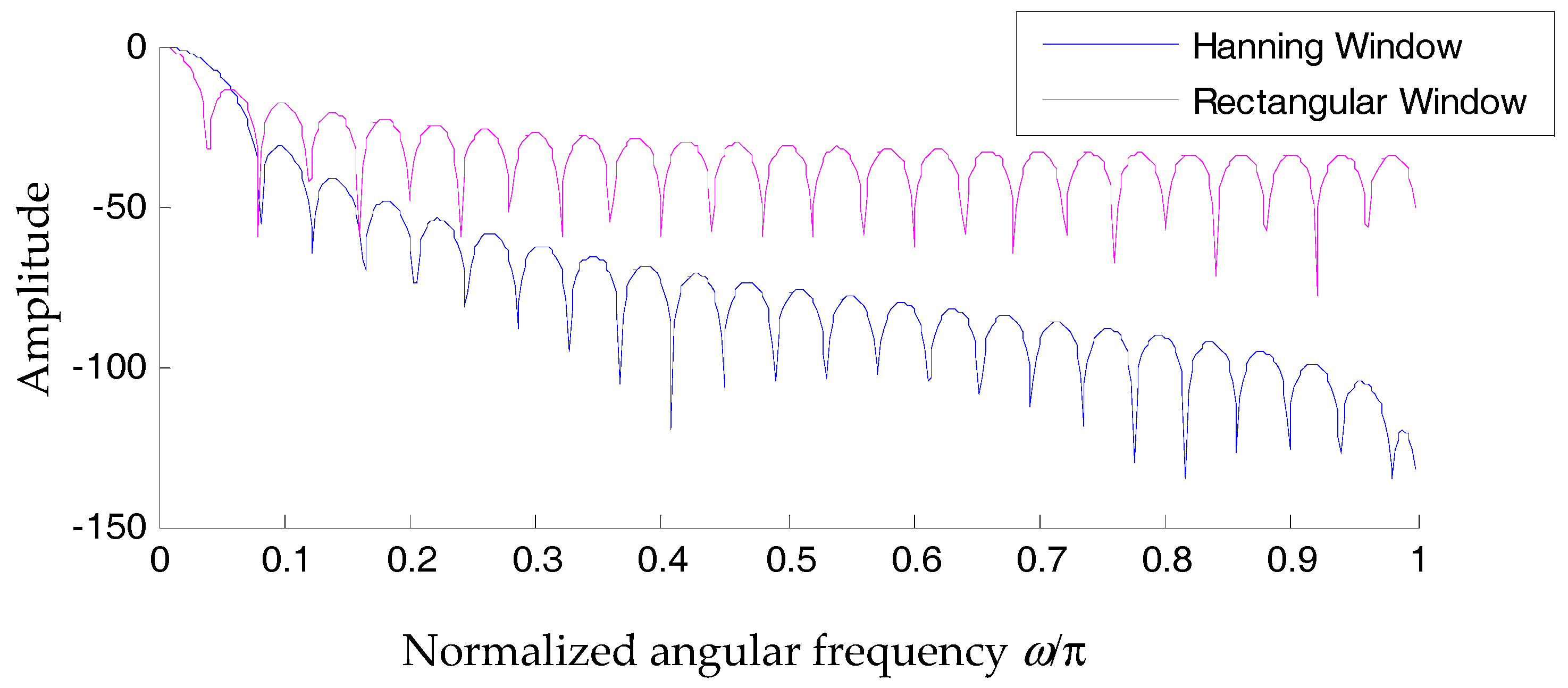
Figure 4.
Comparison between the magnitude spectra of a rectangular window and the Hanning window.
Figure 4.
Comparison between the magnitude spectra of a rectangular window and the Hanning window.
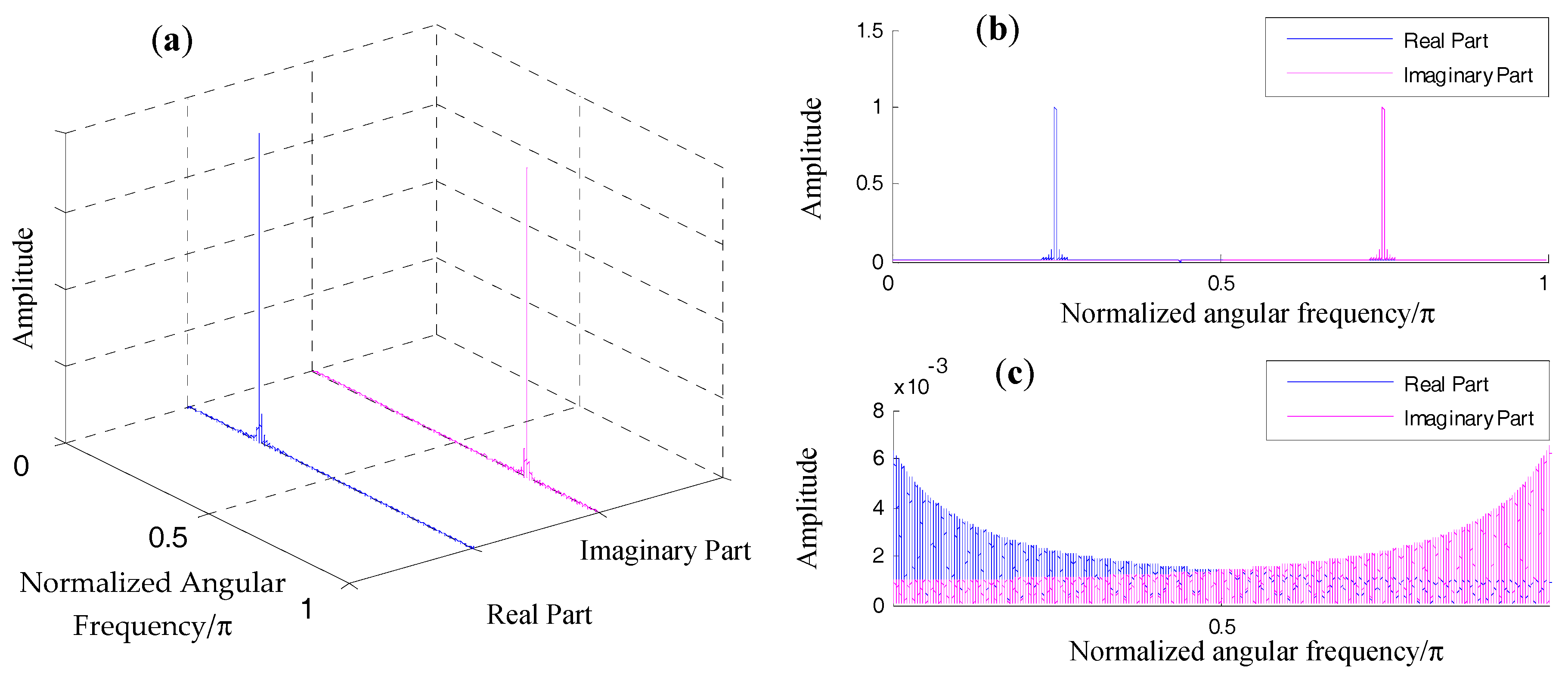
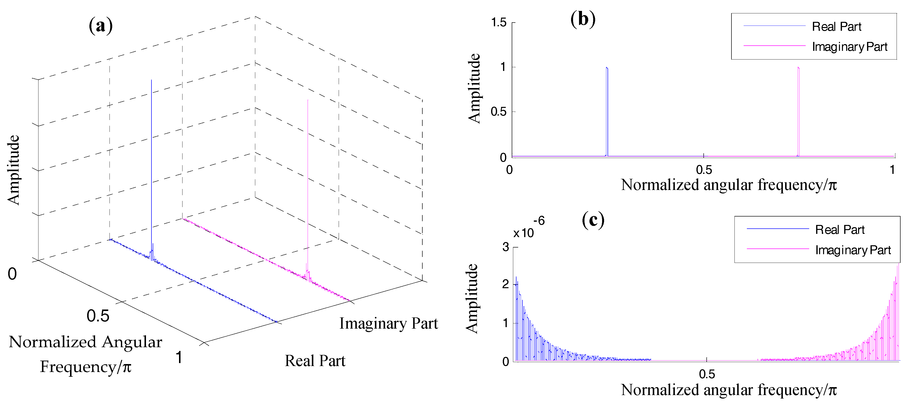
Figure 5.
Demonstration of spectral aliasing of rectangular window: (a) magnitude response of the positive component and the negative component in a 3D coordinate; (b) magnitude response of the positive component and the negative component in a 2D coordinate; (c) zoomed-in plot of (b).
Figure 5.
Demonstration of spectral aliasing of rectangular window: (a) magnitude response of the positive component and the negative component in a 3D coordinate; (b) magnitude response of the positive component and the negative component in a 2D coordinate; (c) zoomed-in plot of (b).
Figure 6.
Demonstration of spectral aliasing of a Hanning window: (a) magnitude response of the positive component and the negative component in a 3D coordinate; (b) magnitude response of the positive component and the negative component in a 2D coordinate; (c) zoomed-in plot of (b).
Figure 6.
Demonstration of spectral aliasing of a Hanning window: (a) magnitude response of the positive component and the negative component in a 3D coordinate; (b) magnitude response of the positive component and the negative component in a 2D coordinate; (c) zoomed-in plot of (b).
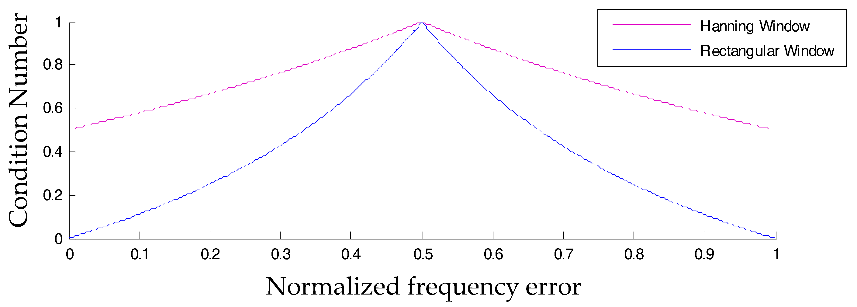
Figure 7.
Condition numbers of rectangular window and Hanning window.
Figure 7.
Condition numbers of rectangular window and Hanning window.
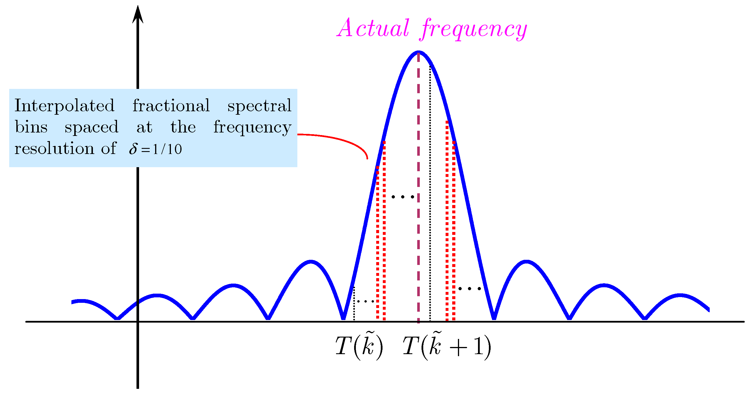
Figure 8.
The interpolated spectral bins around an actual harmonic component.
Figure 8.
The interpolated spectral bins around an actual harmonic component.
Figure 9.
The interpolated spectral bins around an actual harmonic component.
Figure 9.
The interpolated spectral bins around an actual harmonic component.
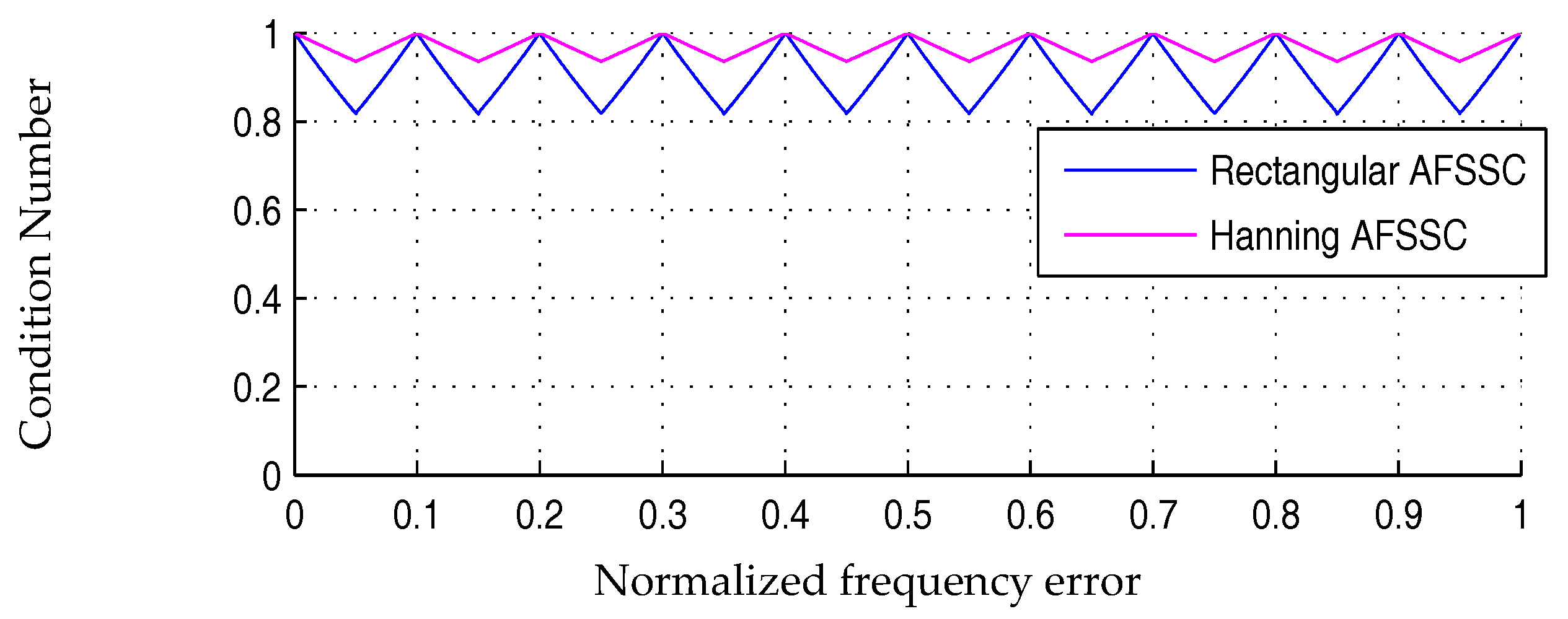
Figure 10.
Condition numbers of rectangular-window-based and Hanning-window-based spectral correction methods enhanced by spectral interpolations.
Figure 10.
Condition numbers of rectangular-window-based and Hanning-window-based spectral correction methods enhanced by spectral interpolations.
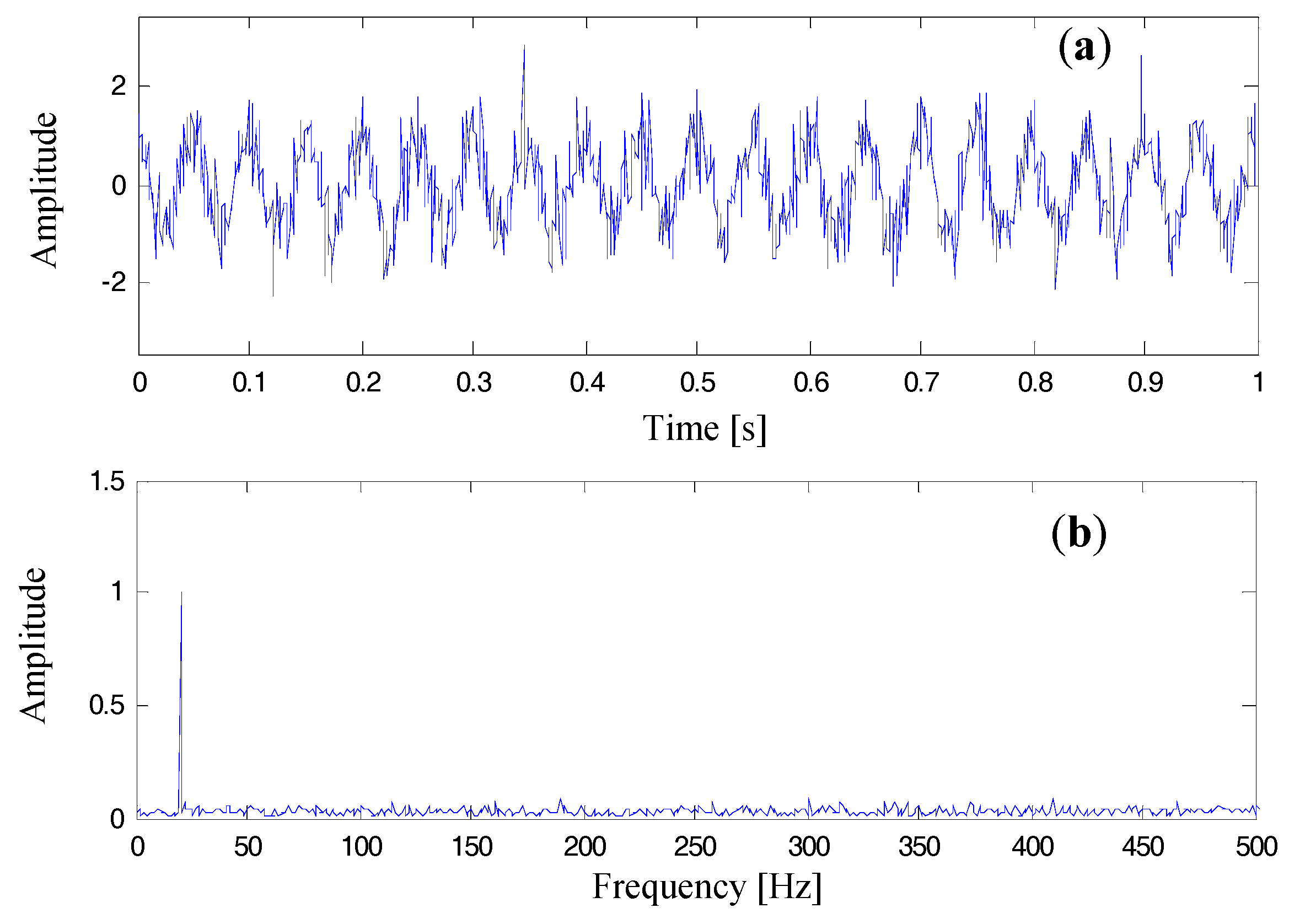
Figure 11.
Plots of the simulated sinusoidal wave corrupted by white Gaussian noise (SNR = 3dB): (a) time domain wave; (b) FFT spectrum.
Figure 11.
Plots of the simulated sinusoidal wave corrupted by white Gaussian noise (SNR = 3dB): (a) time domain wave; (b) FFT spectrum.
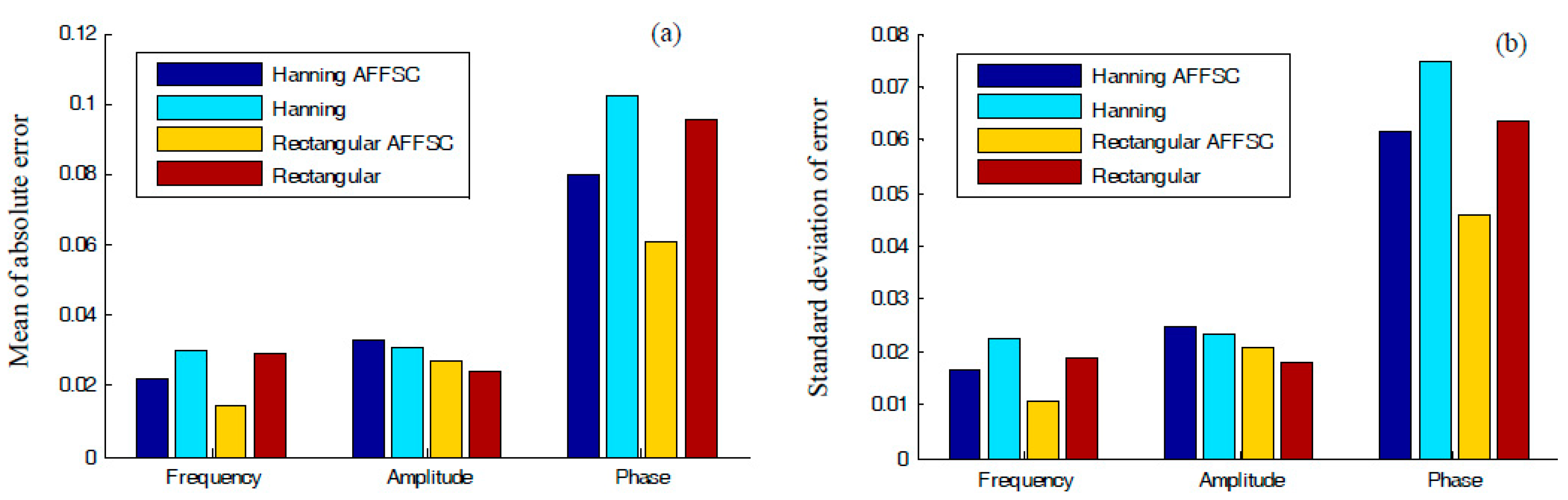
Figure 12.
(a) Mean values of the estimated errors regarding the harmonic information (frequency, amplitude, and phase) using different spectral correction methods, and (b) standard deviations of the estimated errors regarding the harmonic information (frequency, amplitude, and phase) using different spectral correction methods.
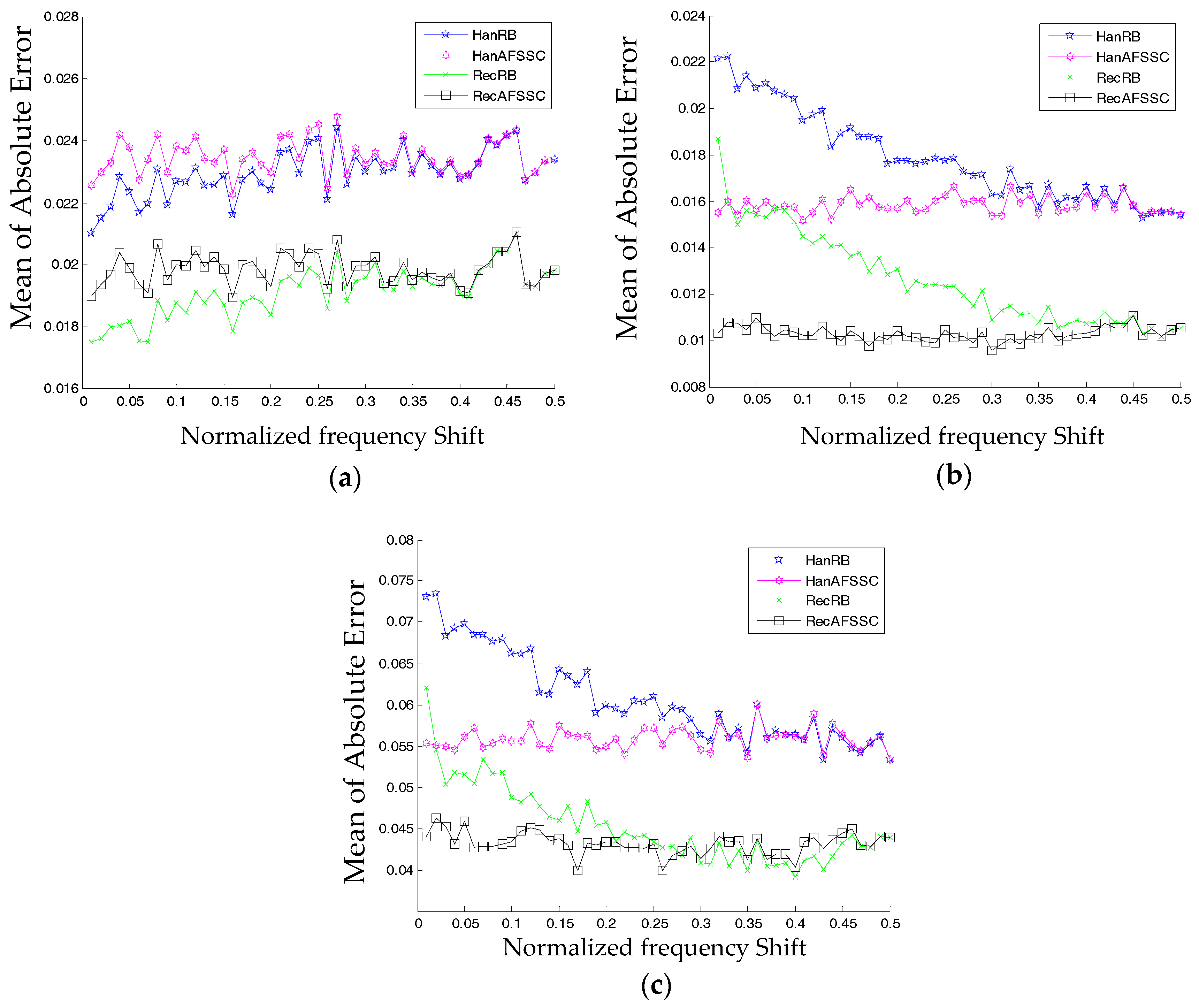
Figure 13.
Comparisons on the comparison of four comparison methods with respect to information of (a) amplitude, (b) frequency, and (c) phase.
Figure 13.
Comparisons on the comparison of four comparison methods with respect to information of (a) amplitude, (b) frequency, and (c) phase.
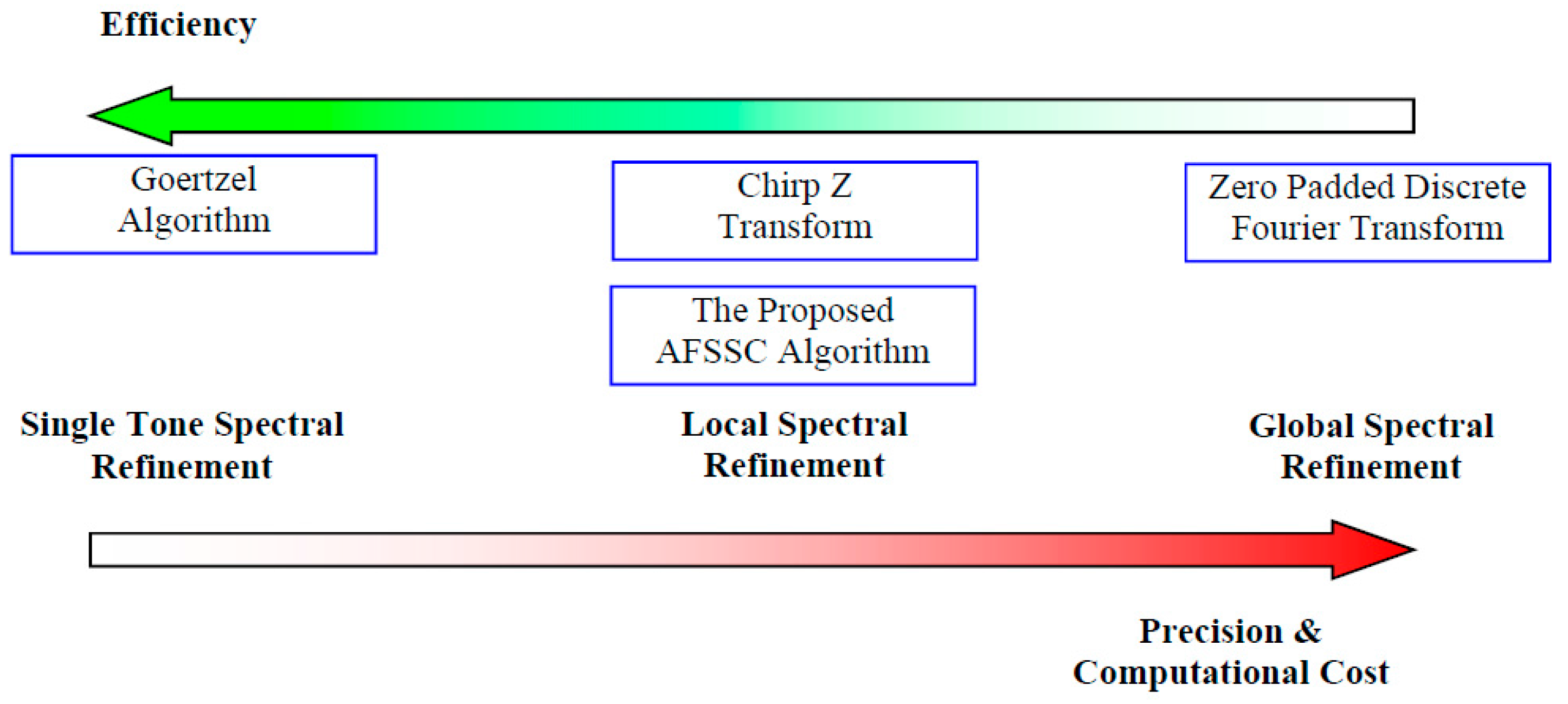
Figure 14.
Pros and cons of some classical spectral refinement techniques with the proposed AFSSC algorithm.
Figure 14.
Pros and cons of some classical spectral refinement techniques with the proposed AFSSC algorithm.
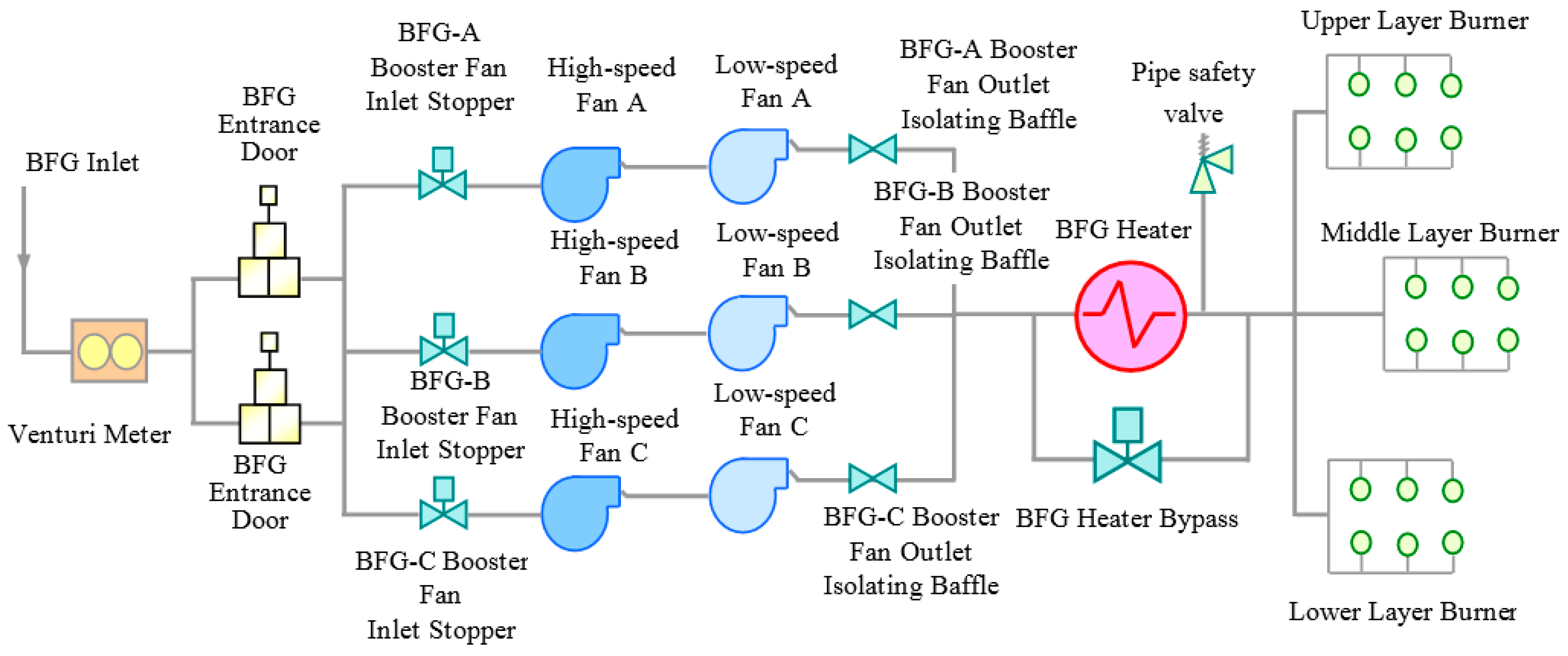
Figure 15.
Schematic diagram of the BFG power plant.
Figure 15.
Schematic diagram of the BFG power plant.
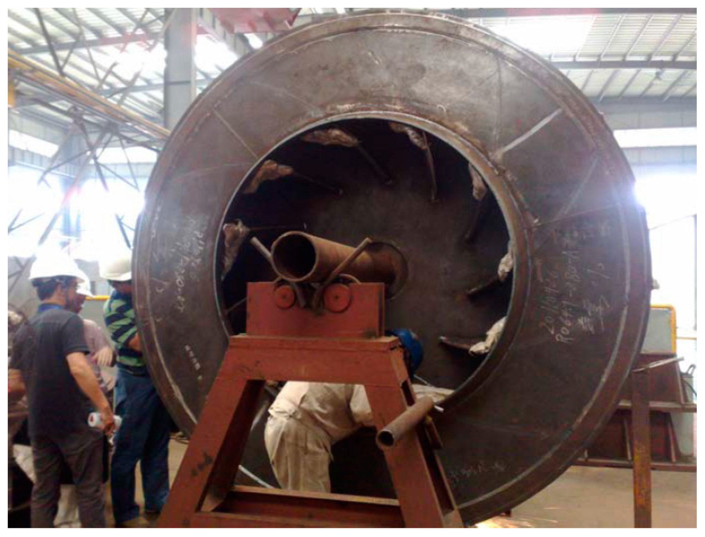
Figure 16.
Photograph of the centrifugal compressor with a fully developed blade crack.
Figure 16.
Photograph of the centrifugal compressor with a fully developed blade crack.
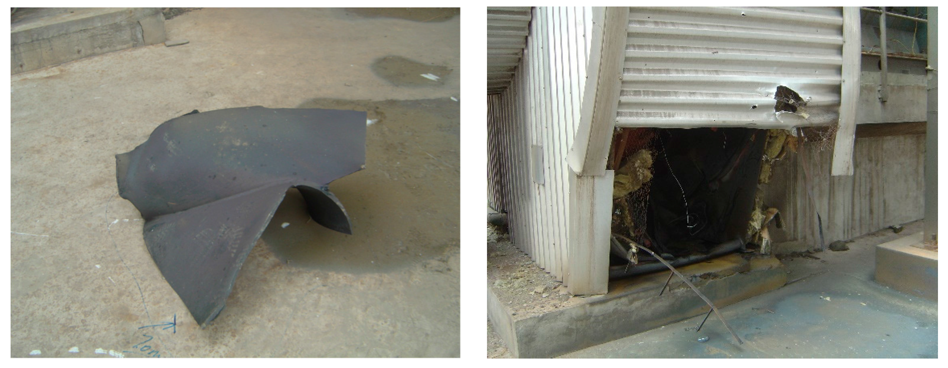
Figure 17.
Photograph of destroyed housing of the BFG booster.
Figure 17.
Photograph of destroyed housing of the BFG booster.
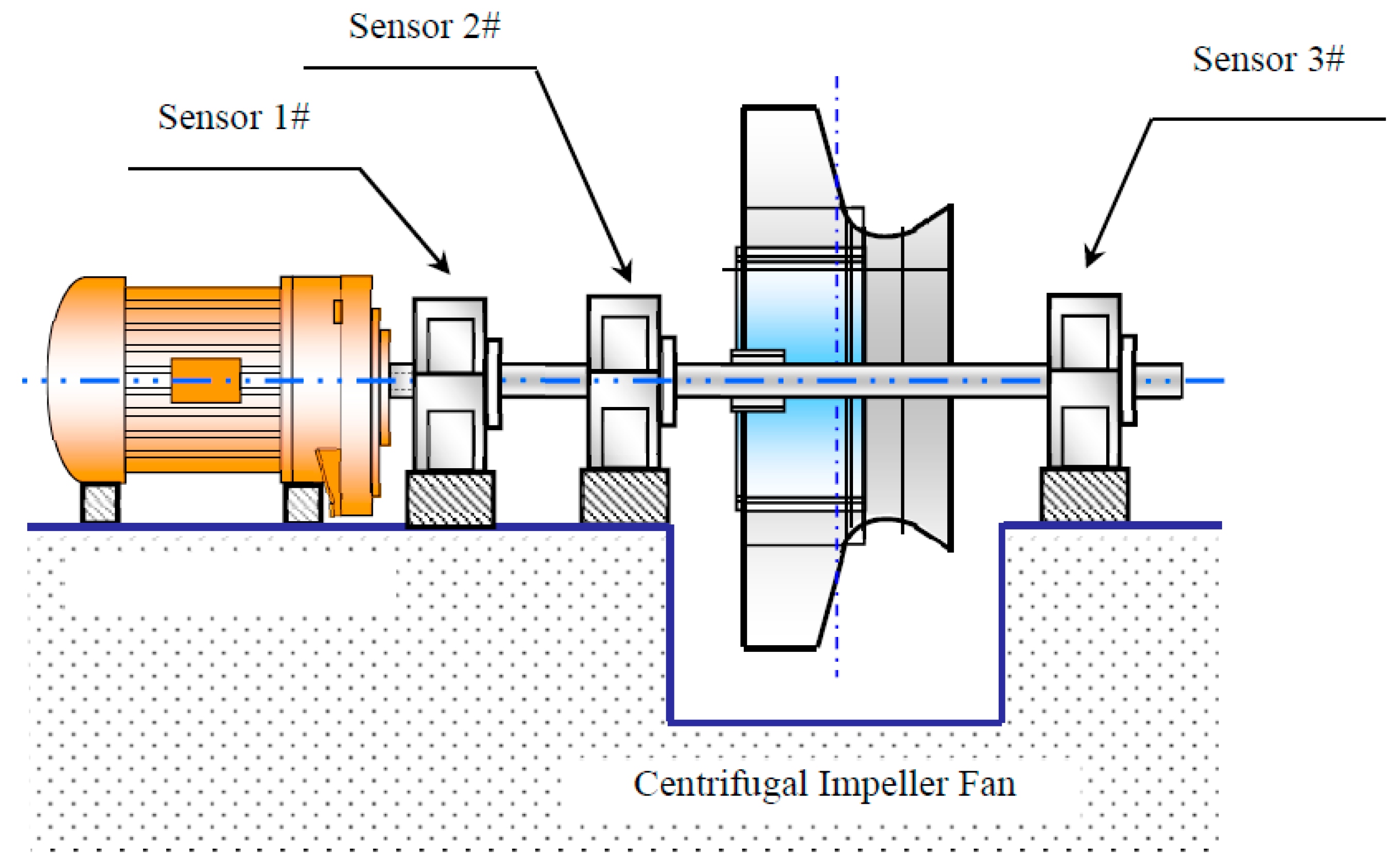
Figure 18.
Mechanical transmission chain of the booster fan (from the driving AC motor to the centrifugal compressor).
Figure 18.
Mechanical transmission chain of the booster fan (from the driving AC motor to the centrifugal compressor).
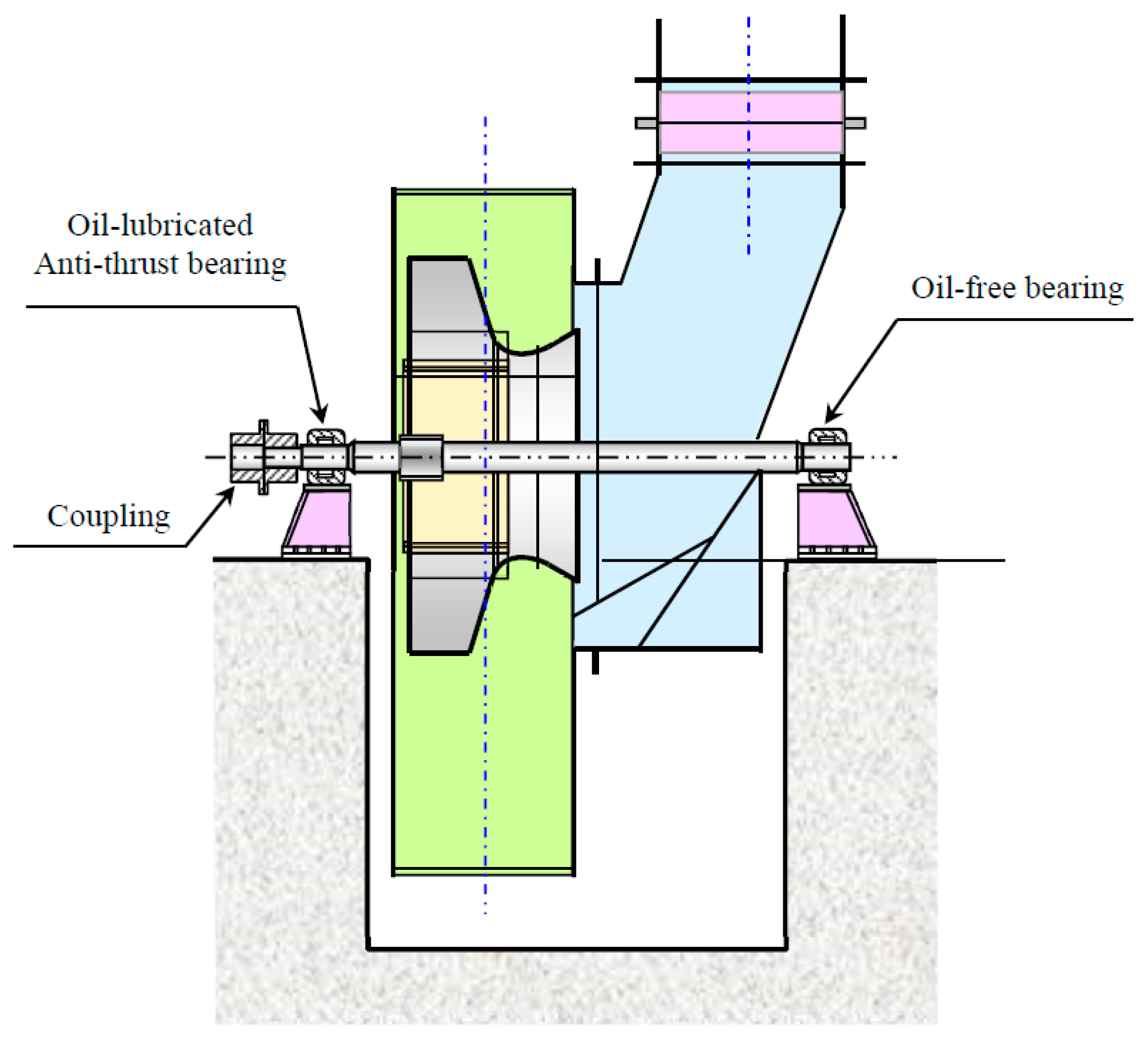
Figure 19.
Detailed schematic diagram of the booster fan and its key component, the centrifugal compressor.
Figure 19.
Detailed schematic diagram of the booster fan and its key component, the centrifugal compressor.
Figure 20.
RMS trends of the centrifugal compressor: (a) Channel ‘2A’, (b) Channel ‘2H’, (c) Channel ‘3A’, and (d) Channel ‘3H’.
Figure 20.
RMS trends of the centrifugal compressor: (a) Channel ‘2A’, (b) Channel ‘2H’, (c) Channel ‘3A’, and (d) Channel ‘3H’.
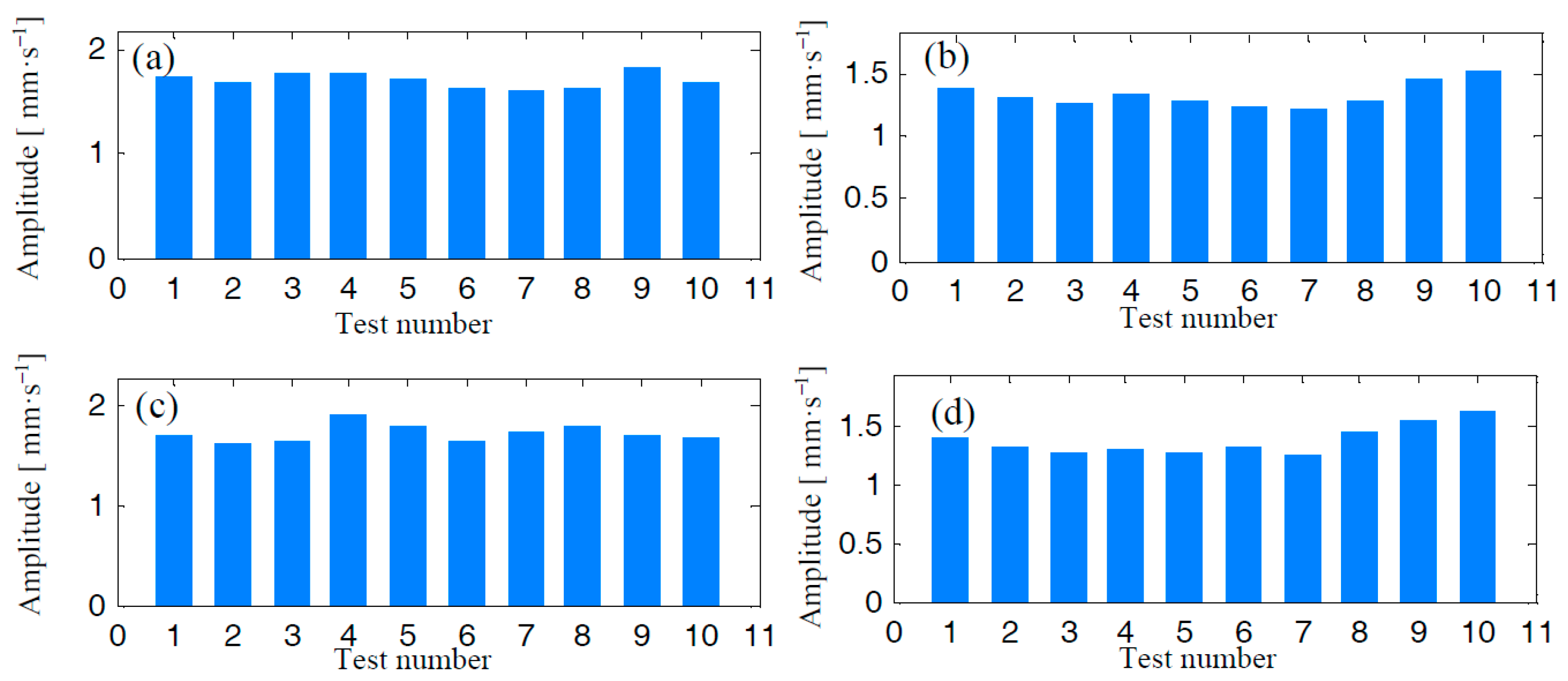
Figure 21.
Kurtosis trends of the centrifugal compressor: (a) Channel ‘2A’, (b) Channel ‘2H’, (c) Channel ‘3A’, and (d) Channel ‘3H’.
Figure 21.
Kurtosis trends of the centrifugal compressor: (a) Channel ‘2A’, (b) Channel ‘2H’, (c) Channel ‘3A’, and (d) Channel ‘3H’.
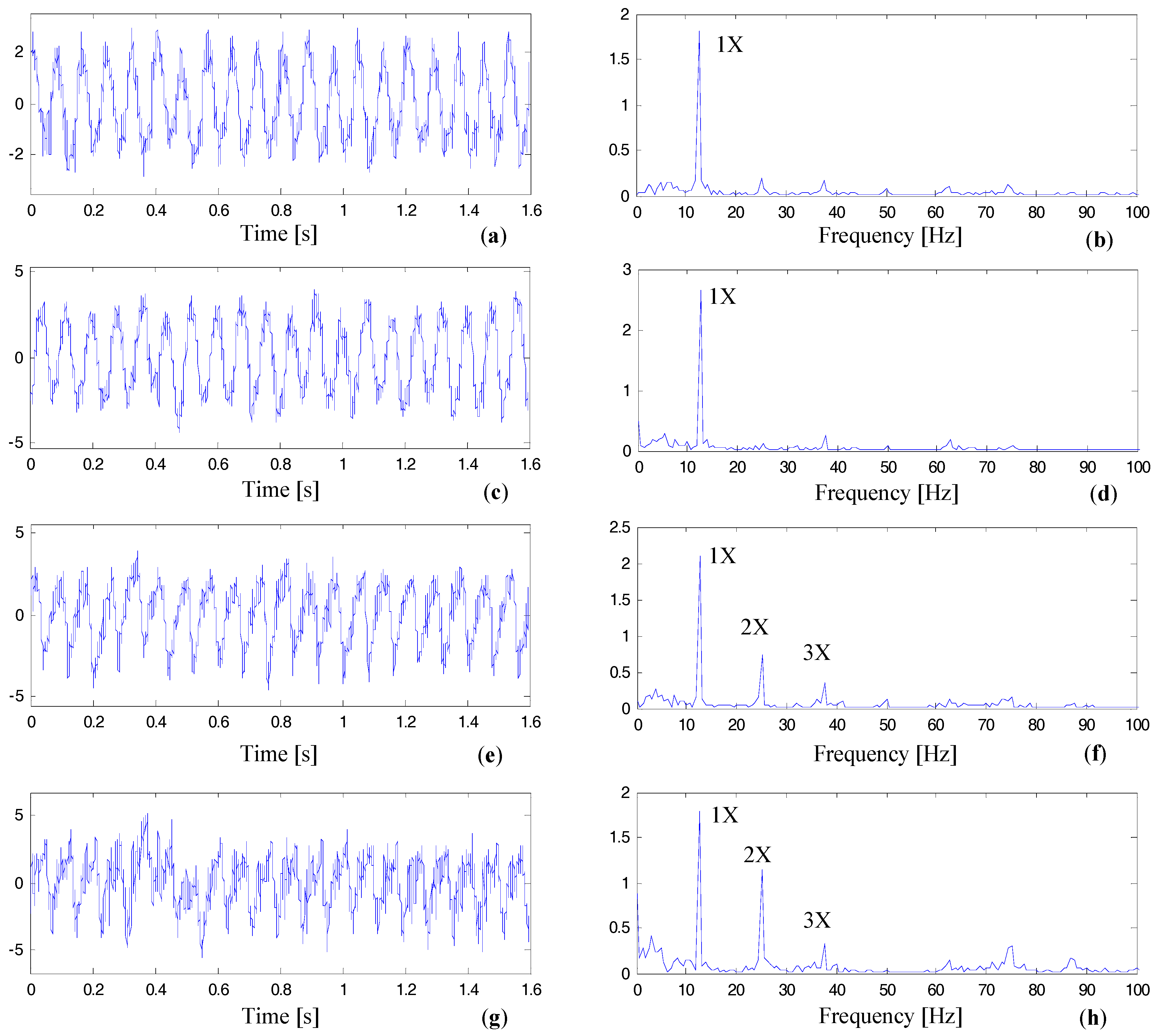
Figure 22.
Time domain waves and FFT spectra of the vibration signal belonging to sensor point 3H: (a) the time domain wave of Test No. 2, (b) Fourier spectra of Test No. 2, (c) the time domain wave of Test No. 4, (d) Fourier spectra of Test No. 8, (e) the time domain wave of Test No. 8, (f) Fourier spectra of Test No. 8, (g) the time domain wave of Test No. 10, (h) Fourier spectra of Test No. 10.
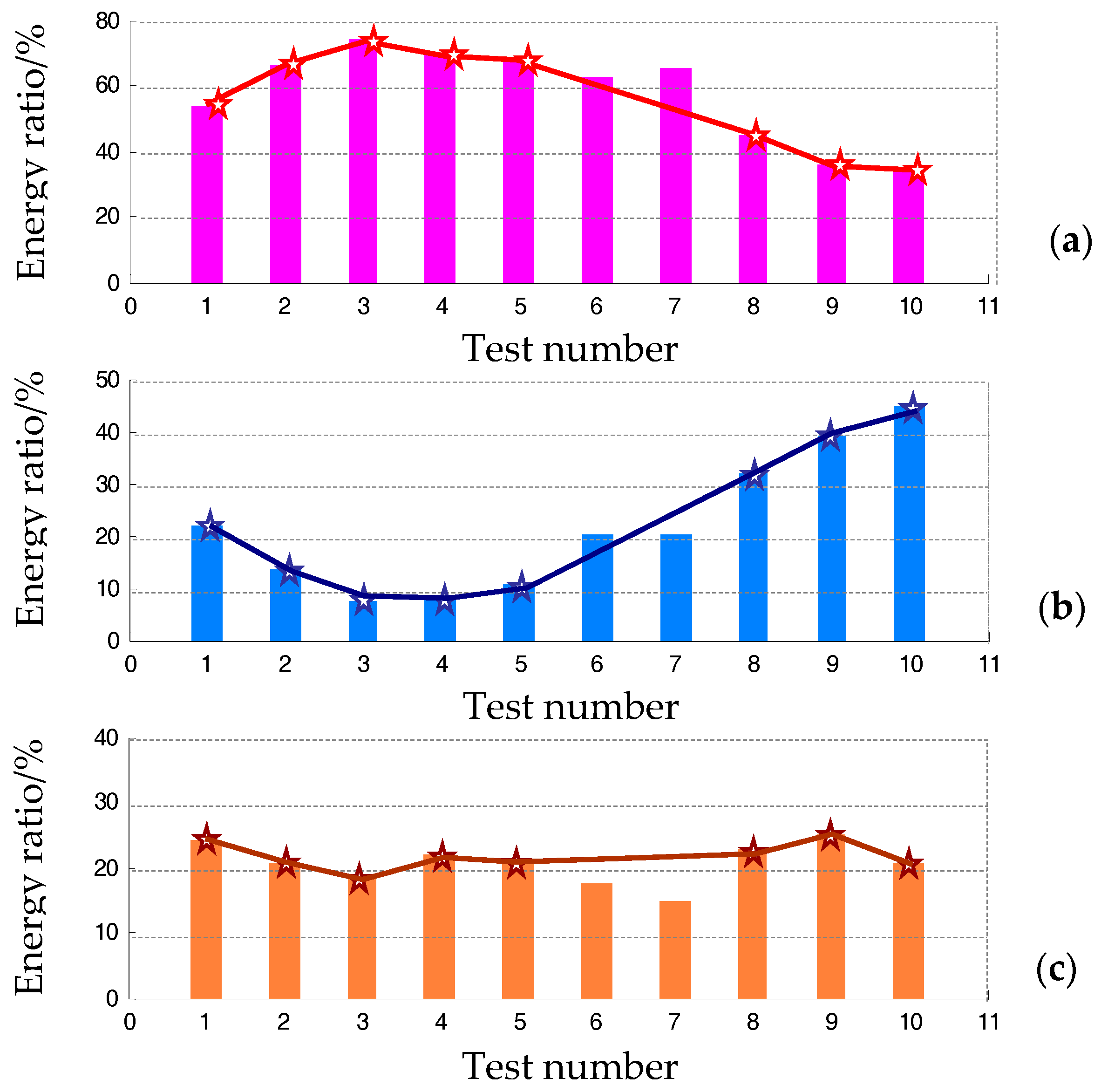
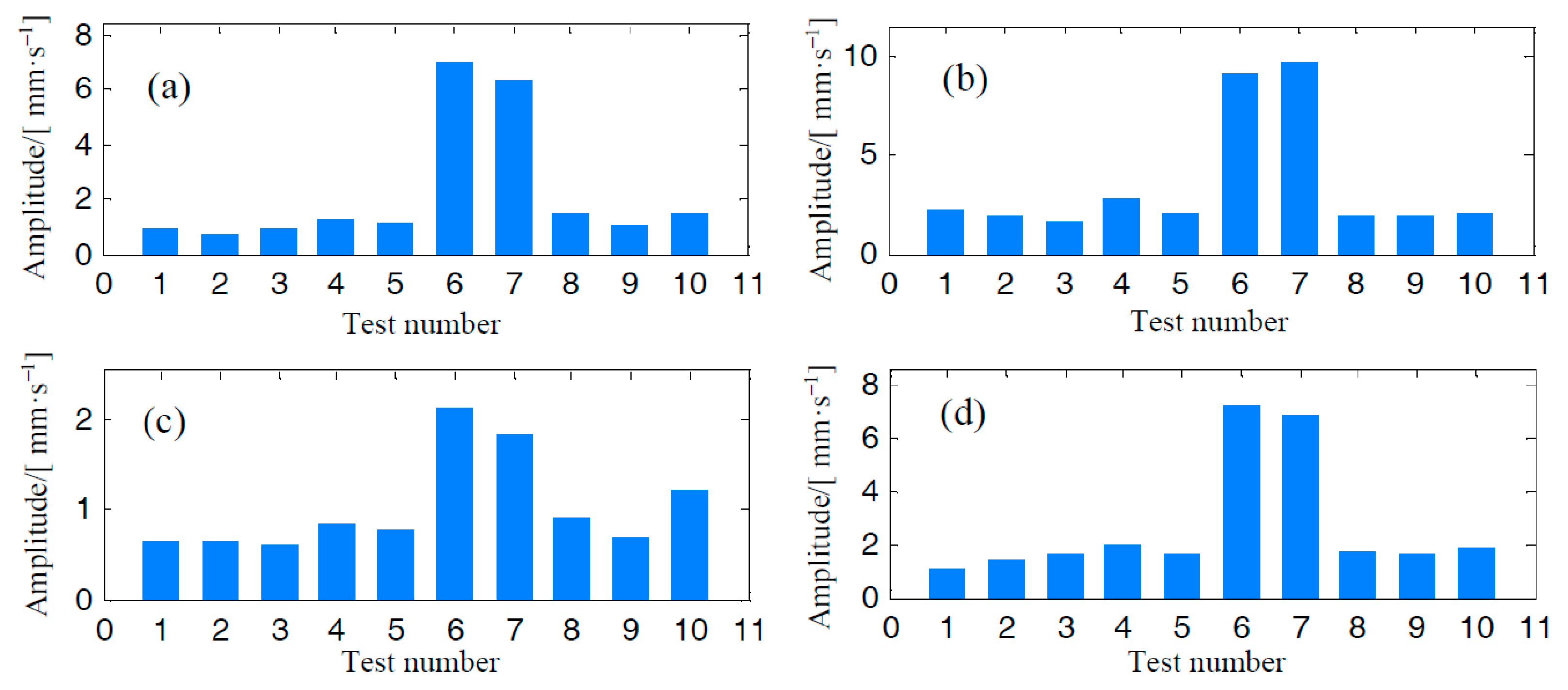
Figure 23.
Energy weight of the three harmonic tones of the fundamental working frequency: (a) the first order, (b) the second order, and (c) the third order.
Figure 23.
Energy weight of the three harmonic tones of the fundamental working frequency: (a) the first order, (b) the second order, and (c) the third order.
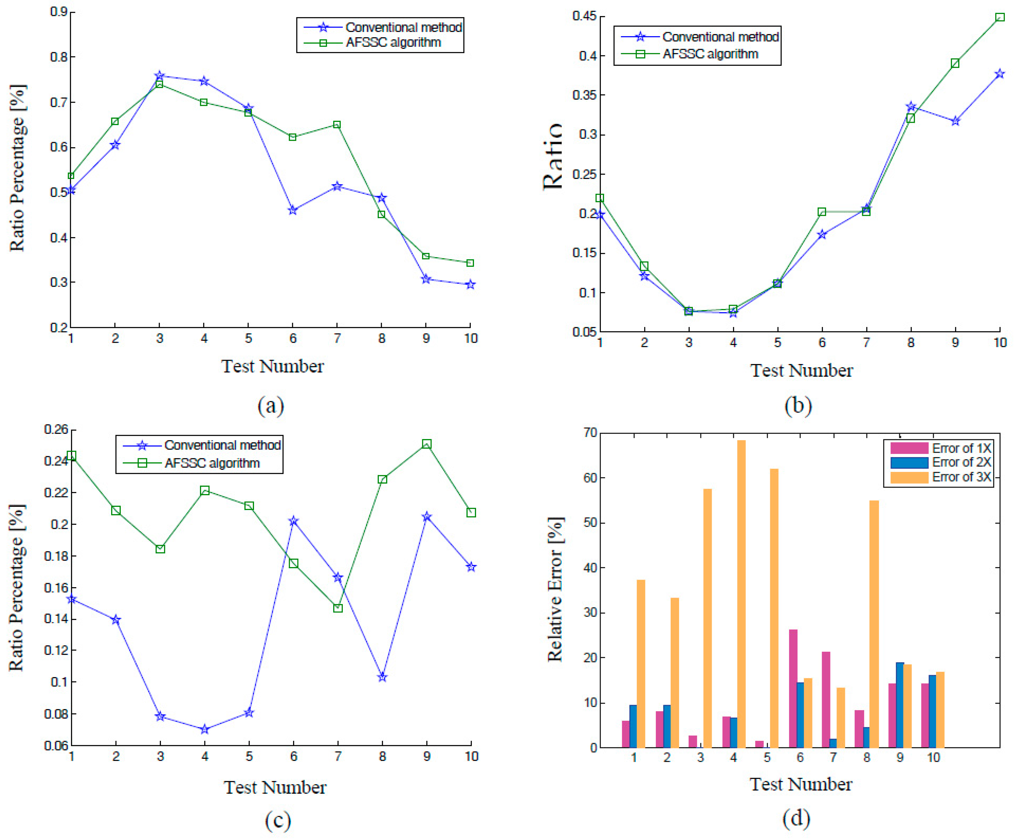
Figure 24.
Comparison between the results of AFSSC and those of FFT: the first order, (b) the second order, and (c) the third order; and (d) curves of relative errors of each harmonic tone in each test.
Figure 24.
Comparison between the results of AFSSC and those of FFT: the first order, (b) the second order, and (c) the third order; and (d) curves of relative errors of each harmonic tone in each test.
Table 1.
Abbreviations of the proposed method and those of four comparison methods.
Table 1.
Abbreviations of the proposed method and those of four comparison methods.
| Abbreviations | Contents |
|---|
| HanRB | Ratio-based spectral correction technique using Hanning window. |
| HanAFSSC | HanRB using active frequency shifting operations as a preprocessing step. |
| RecRB | Ratio-based spectral correction technique using rectangular window. |
| RecAFSSC | RecRB using active frequency shifting operations as a pre-processing step. |
| AFSSC | The proposed method. |
Table 2.
Comparisons of the four techniques when .
Table 2.
Comparisons of the four techniques when .
| Spectral Information | HanAFSSC | HanRB | RecAFSSC | RecRB |
|---|
| Frequency (Hz) | Mean | 0.0228 | 0.0282 | 0.0149 | 0.0209 |
| Std. | 0.0168 | 0.0207 | 0.0113 | 0.0149 |
| Amplitude | Mean | 0.0325 | 0.0312 | 0.0274 | 0.0252 |
| Std. | 0.0246 | 0.0235 | 0.0209 | 0.0195 |
| Phase (rad) | Mean | 0.0789 | 0.0926 | 0.0614 | 0.0715 |
| Std. | 0.0593 | 0.0690 | 0.0468 | 0.0528 |
Table 3.
Comparisons of the four techniques when .
Table 3.
Comparisons of the four techniques when .
| Spectral Information | HanAFSSC | HanRB | RecAFSSC | RecRB |
|---|
| Frequency | Mean | 0.0232 | 0.0304 | 0.0148 | 0.0210 |
| Std. | 0.0161 | 0.0218 | 0.0114 | 0.0153 |
| Amplitude | Mean | 0.0324 | 0.0306 | 0.0278 | 0.0251 |
| Std. | 0.0248 | 0.0232 | 0.0209 | 0.0188 |
| Phase | Mean | 0.0797 | 0.0990 | 0.0637 | 0.0709 |
| Std. | 0.0555 | 0.0717 | 0.0543 | 0.0581 |
Table 4.
Comparisons of the four techniques when .
Table 4.
Comparisons of the four techniques when .
| Spectral Information | HanAFSSC | HanRB | RecAFSSC | RecRB |
|---|
| Frequency | Mean | 0.0262 | 0.0302 | 0.0154 | 0.0284 |
| Std. | 0.0173 | 0.0238 | 0.0113 | 0.0193 |
| Amplitude | Mean | 0.0325 | 0.0305 | 0.0280 | 0.0259 |
| Std. | 0.0234 | 0.0221 | 0.0204 | 0.0185 |
| Phase | Mean | 0.0829 | 0.1025 | 0.0648 | 0.0926 |
| Std. | 0.0622 | 0.0791 | 0.0488 | 0.0642 |
Table 5.
Information of the 10 historical vibration tests (date, rotation speed, units).
Table 5.
Information of the 10 historical vibration tests (date, rotation speed, units).
| Test Number | Interval (Days) | Sensors on Bearing Shell 2# | Sensors on Bearing Shell 3# | Remarks |
|---|
| Axial (mm/s) | Horizon (mm/s) | Vertical (GE) | Axial (mm/s) | Horizon (mm/s) | Vertical (GE) |
|---|
| 1 | - | L | L | L | L | L | L | Low speed operations (1-The initial test’) |
| 2 | 99 | L | L | L | L | L | L |
| 3 | 62 | L | L | L | L | L | L |
| 4 | 35 | L | L | L | L | L | L |
| 5 | 54 | L | L | L | L | L | L |
| 6 | 29 | H | H | H | H | H | H | High speed operations |
| 7 | 5 | H | H | H | H | H | H |
| 8 | 30 | L | L | L | L | L | L | Low speed operations |
| 9 | 29 | L | L | L | L | L | L |
| 10 | 27 | L | L | L | L | L | L |
Table 6.
Corrected information of frequency, amplitude, and phase using the proposed AFSSC.
Table 6.
Corrected information of frequency, amplitude, and phase using the proposed AFSSC.
| Test Number | Fundamental Frequency | Fundamental Frequency | Fundamental Frequency |
|---|
| Amplitude (mm·s−1) | Phase (°) | Amplitude (mm·s−1) | Phase (°) | Amplitude (mm·s−1) | Phase (°) |
|---|
| 1 | 1.316 | 136.065 | 0.269 | −33.388 | 0.199 | 125.074 |
| 2 | 1.844 | −33.603 | 0.187 | −71.140 | 0.195 | −4.870 |
| 3 | 2.180 | 158.022 | 0.112 | −63.192 | 0.181 | −150.955 |
| 4 | 2.670 | −173.618 | 0.151 | −6.510 | 0.282 | 20.693 |
| 5 | 2.252 | 47.781 | 0.185 | 104.608 | 0.235 | −110.818 |
| 6 | 9.590 | −43.643 | 1.558 | −49.710 | 0.900 | 62.944 |
| 7 | 9.372 | −63.354 | 1.460 | −101.821 | 0.706 | −26.358 |
| 8 | 2.110 | −45.932 | 0.752 | 153.325 | 0.357 | −31.131 |
| 9 | 1.884 | 63.890 | 1.027 | 6.055 | 0.440 | −50.505 |
| 10 | 1.795 | −162.645 | 1.171 | −91.907 | 0.361 | 1.491 |


