
Deformation Study of Lean Methane-Air Premixed Spherically Expanding Flames under a Negative Direct Current Electric Field


Abstract
:
1. Introduction
2. Experimental Set up
2.1. Experimental Apparatus
2.2. Experimental Process
3. Numerical Set up
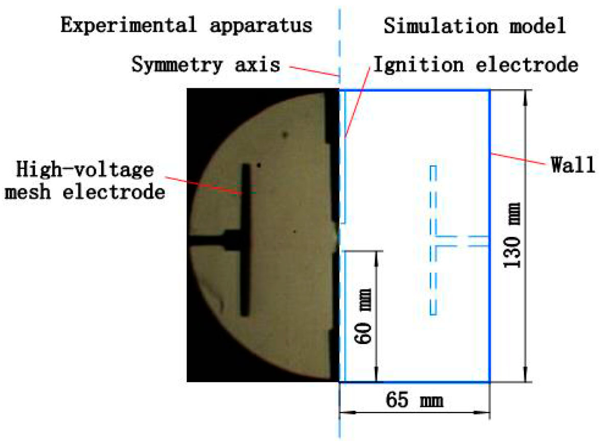
3.1. Geometry
3.2. Numerical Assumption
3.3. Governing Equations
3.4. Reaction Mechanism
3.5. Boundary Conditions
4. Result and Discuss
4.1. Flame Shape and Propagation Speed
4.2. Explanation of Flame Deformation
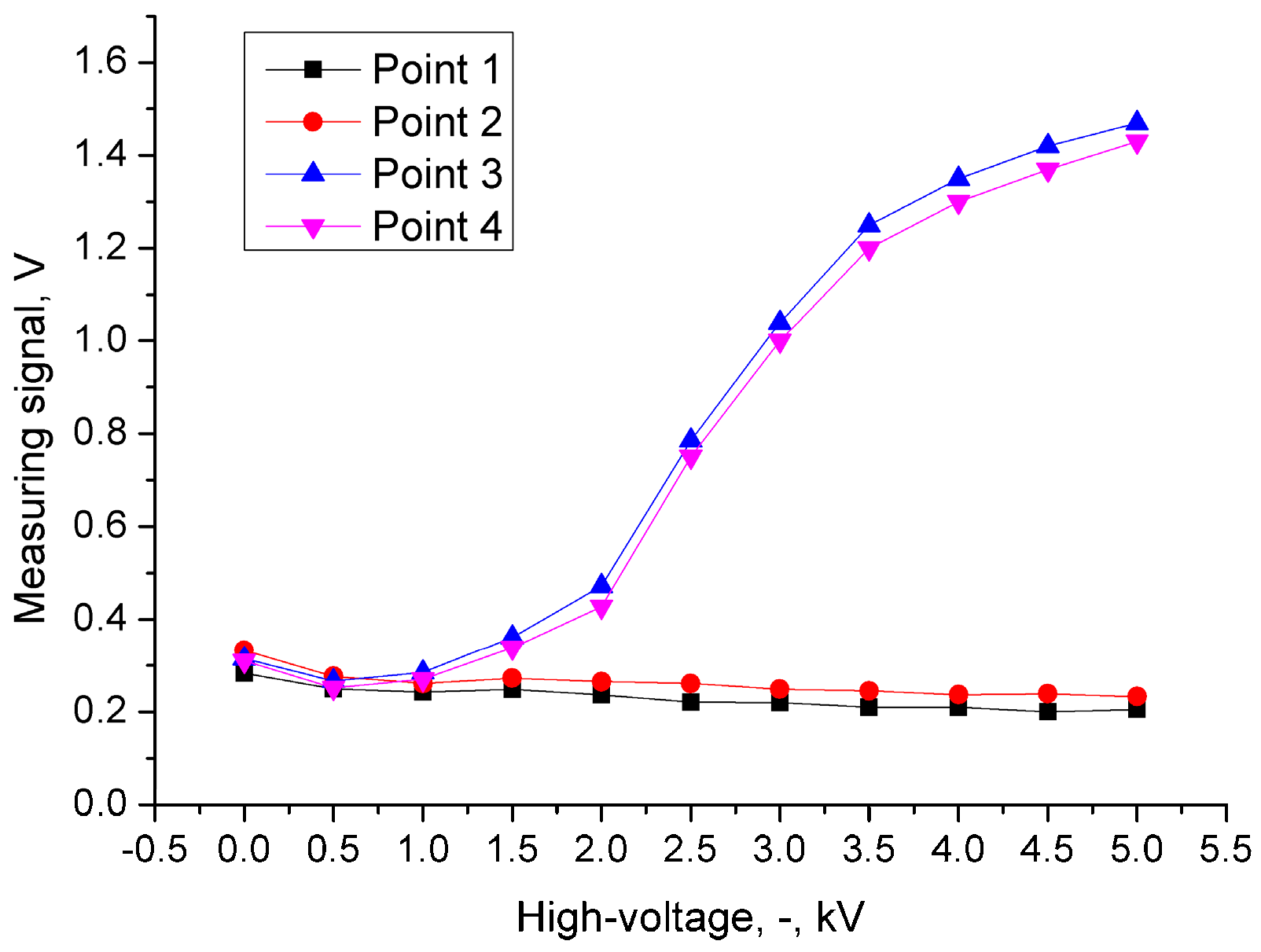
4.3. Ionic Concentration Distribution
5. Conclusions
- (1)
- The simulation method of adding an extra electric body force to the positive ions could make a good prediction for the negative DC electric field acting on the spherically expanding flame, including the flame shape, flame propagation speed and some special flame structure.
- (2)
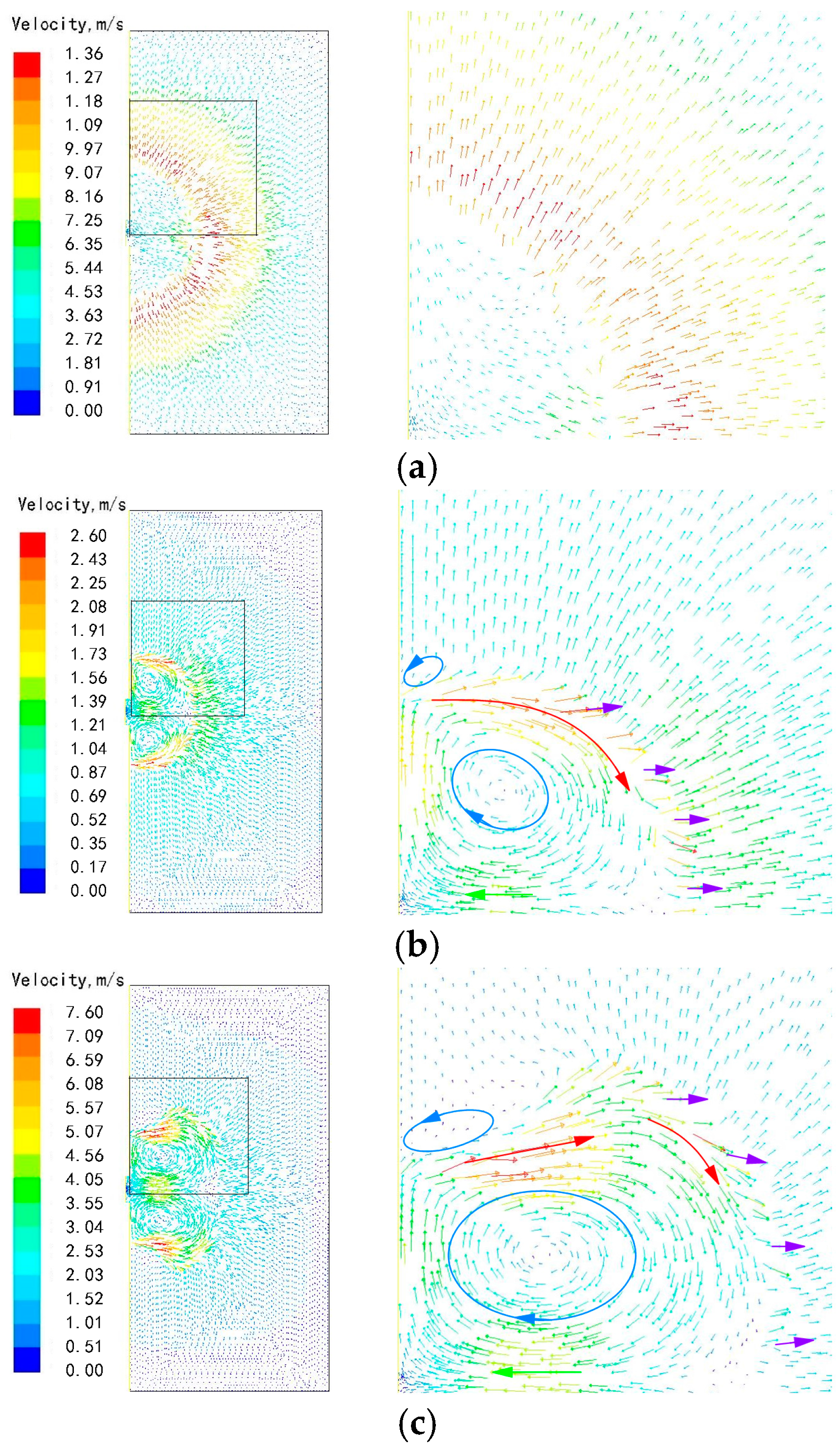
- When a negative DC electric field was applied on a spherically expanding flame, a small part of the ions and other neutral molecules on the flame surface would be driven to the premixed zone by the electric field, and then promote the flame propagation in the electric field direction. Besides, the majority of ions and neutral molecules will form an ionic flow moving along the flame surface. This kind of ionic flow was usually formed on the upper and lower sides of the flame surface by the superposition effect of the electric field force and the aerodynamic drag, and it will lead to a non-uniform ionic concentration distribution on the flame surface.
- (3)
- The ionic flow along the flame surface would induce two vortexes both inside and outside of the flame surface due to the viscosity. The outside vortex would obviously inhibit the flame propagation in the vertical direction by entraining the premixed gas into the flame surface and take away the heat from the flame surface, while, the inside vortex would induce a secondary inward flow and then change the flame shape, even forming a pit structure at the center position.
Acknowledgments
Author Contributions
Conflicts of Interest
Nomenclature
| E | electrical field intensity |
| H | static enthalpy |
| K | mobility |
| ci | concentration of ions |
| p | pressure |
| Q | heat release |
| S | source term |
| t | time |
| T | temperature |
| q | element charge |
| u | horizontal velocity |
| v | vertical velocity |
| Φ | viscous dissipative term |
| λ | thermal conductivity |
| ν | dynamic viscosity |
| ρ | density |
| rh, rv | flame radius in horizontal and vertical direction |
| vh, vv | flame propagation speed in horizontal and vertical direction |
| au | uniform coefficient of the electric field |
| as | modified factor of effective section area of the Langmuir probe |
References
- Kim, W.; Do, H.; Mungal, M.G.; Cappelli, M.A. Optimal discharge placement in plasma-assisted combustion of a methane jet in cross flow. Combust. Flame 2008, 153, 603–615. [Google Scholar] [CrossRef]
- Ombrello, T.; Won, S.H.; Ju, Y. Flame propagation enhancement by plasma excitation of oxygen. Part I: Effects of O3. Combust. Flame 2010, 157, 1906–1915. [Google Scholar]
- Ombrello, T.; Won, S.H.; Ju, Y. Flame propagation enhancement by plasma excitation of oxygen. Part II: Effects of O2(a1Δg). Combust. Flame 2010, 157, 1916–1928. [Google Scholar] [CrossRef]
- Tao, R.; Huang, K.; Tang, H.; Bell, D. Electrorheology leads to efficient combustion. Energy Fuels 2008, 22, 3785–3788. [Google Scholar] [CrossRef]
- Cha, M.S.; Lee, S.M.; Kim, K.T.; Chung, S.H. Soot suppression by nonthermal plasma in coflow jet diffusion flames using a dielectric barrier discharge. Combust. Flame 2005, 141, 438–447. [Google Scholar] [CrossRef]
- Vega, E.V.; Shin, S.S.; Lee, K.Y. NO emission of oxygen-enriched CH4/O2/N2 premixed flames under electric field. Fuel 2007, 86, 512–519. [Google Scholar] [CrossRef]
- Zhang, Y.; Wu, Y.; Yang, H. Effect of high-frequency alternating electric fields on the behavior and nitricoxide emission of laminar non-premixed flames. Fuel 2013, 109, 350–355. [Google Scholar] [CrossRef]
- Altendorfner, F.; Kuhl, J.; Zigan, L. Study of the influence of electric fields on flames using planar LIF and PIV techniques. Proc. Combust. Inst. 2011, 33, 3195–3201. [Google Scholar] [CrossRef]
- Hu, J.; Rivin, B.; Sher, E. The effect of an electric field on the shape of co-flowing and candle-type methane–air flames. Exp. Therm. Fluid Sci. 2000, 21, 124–133. [Google Scholar] [CrossRef]
- Vega, E.V.; Lee, K.Y. An experimental study on laminar CH4/O2/N2 premixed flames under an electric field. J. Mech. Sci. Technol. 2008, 22, 312–319. [Google Scholar] [CrossRef]
- Wisman, D.L.; Marcum, S.D.; Ganguly, B.N. Electrical control of the thermo diffusive instability in premixed propane-air flames. Combust. Flame 2007, 151, 639–648. [Google Scholar] [CrossRef]
- Ata, A.; Cowart, J.S.; Vranos, A.; Cetegen, B.M. Effects of direct current electric field on the blow off characteristics of bluff-body stabilized conical premixed flames. Combust. Sci. Technol. 2005, 177, 1291–1304. [Google Scholar] [CrossRef]
- Marcum, S.D.; Ganguly, B.N. Electric-field-induced flame speed modification. Combust. Flame 2005, 143, 27–36. [Google Scholar] [CrossRef]
- Sakhrieh, A.; Lins, G.; Dinkelacker, F.; Hammer, T.; Leipertz, A.; Branston, D.W. The influence of pressure on the control of premixed turbulent flames using an electric field. Combust. Flame 2005, 143, 313–322. [Google Scholar] [CrossRef]
- Kim, M.K.; Chung, H.S.; Kim, H.H. Effect of electric fields on the stabilization of premixed laminar Bunsen flames at low AC frequency: Bi-ionic wind effect. Combust. Flame 2012, 159, 1151–1159. [Google Scholar] [CrossRef]
- Lee, S.M.; Park, C.S.; Cha, M.S.; Chung, S.H. Effect of electric fields on the liftoff of non-premixed turbulent jet flames. IEEE Trans. Plasma Sci. 2005, 33, 1703–1709. [Google Scholar]
- Borgatelli, F.; Dunn-Rankin, D. Behavior of a small diffusion flame as an electrically active component in a high-voltage circuit. Combust. Flame 2012, 159, 210–220. [Google Scholar] [CrossRef]
- Volkov, E.N.; Sepman, A.V.; Kornilov, V.N.; Konnov, A.A.; Shoshin, Y.S.; de Coey, L.P.H. Towards the mechanism of DC electric field effect on flat premixed flame. In Proceedings of the European Combustion Meeting, Vienna, Austria, 14–17 April 2009.
- Vandenboom, J.; Konnov, A.; Verhasselt, A.; Kornilov, V.; Degoey, L.; Nijmeijer, H. The effect of a DC electric field on the laminar burning velocity of premixed methane/air flames. Proc. Combust. Inst. 2009, 32, 1237–1244. [Google Scholar] [CrossRef]
- Sanchez-Sanz, M.; Murphy, D.C.; Fernandez-Pello, C. Effect of an external electric field on the propagation velocity of premixed flames. Proc. Combust. Inst. 2015, 35, 3463–3470. [Google Scholar] [CrossRef]
- Stockman, E.S.; Zaidi, S.H.; Miles, R.B.; Carter, C.D.; Ryan, M.D. Measurements of combustion properties in a microwave enhanced flame. Combust. Flame 2009, 156, 1453–1461. [Google Scholar] [CrossRef]
- Prager, J.; Riedel, U.; Warnatz, J. Modeling ion chemistry and charged species diffusion in lean methane–oxygen flames. Proc. Combust. Inst. 2007, 31, 1129–1137. [Google Scholar] [CrossRef]
- Patyal, A.; Kyritsis, D.; Matalon, M. Electric field effects in the presence of chemi-ionization on droplet burning. Combust. Flame 2016, 164, 99–110. [Google Scholar] [CrossRef]
- Dayal, S.K.; Pandya, T.P. Structure of counterflow diffustion flame in transverse electric fields. Combust. Flame 1979, 35, 277–287. [Google Scholar] [CrossRef]
- Xie, L.; Kishi, T.; Kono, M. The influence of electric fields on soot formation and flame structure of diffusion flames. J. Therm. Sci. 1993, 2, 288–293. [Google Scholar] [CrossRef]
- Cha, M.S.; Lee, Y. Premixed combustion under electric field in a constant volume chamber. IEEE Trans. Plasma Sci. 2012, 40, 3131–3138. [Google Scholar] [CrossRef]
- Meng, X.W.; Wu, X.M.; Kang, C.; Tang, A.D.; Gao, Z.Q. Effects of direct-current (DC) electric fields on flame propagation and combustion characteristics of premixed CH4/O2/N2 flames. Energy Fuels 2012, 26, 6612–6620. [Google Scholar]
- Yamashita, K.; Karnani, S.; Dunn-Rankin, D. Numerical prediction of ion current from a small methane jet flame. Combust. Flame 2009, 156, 1227–1233. [Google Scholar] [CrossRef]
- Ulybyshev, K.E. Calculation of the effect of a constant electric field on the gas dynamics and nitrogen oxide emission in laminar diffusion flame. Fluid Dyn. 2000, 35, 38–42. [Google Scholar] [CrossRef]
- Duan, H.; Wu, X.M.; Zhang, C.; Cui, Y.C.; Hou, J.C.; Li, C.; Gao, Z.Q. Experimental study of lean premixed CH4/N2/O2 flames under high frequency alternating-current electric fields. Energy Fuels 2015, 29, 7601–7611. [Google Scholar] [CrossRef]
- Duan, H.; Wu, X.M.; Sun, T.Q.; Liu, B.; Fang, J.F.; Li, C.; Gao, Z.Q. Effects of electric field intensity and distribution on flame propagation speed of CH4/O2/N2 flames. Fuel 2015, 158, 807–815. [Google Scholar] [CrossRef]
- Jacobs, S.V.; Xu, K.G. Examination of ionic wind and cathode sheath effects in a E-field premixed flame with ion density measurements. Phys. Plasmas 2016, 23. [Google Scholar] [CrossRef]
- Han, J.; Casey, T.; Belhi, M.; Arias, P.G.; Bisetti, F.; Im, H.G.; Chen, J.Y. Modeling of the effect of an electric field on the distribution of charged species in 1D premixed flames. In Proceedings of the 10th Asia-Pacific Conference on Combustion, Beijing, China, 19–22 July 2015.
- Goodings, J.M.; Bohme, D.K.; Ng, C.W. Detailed ion chemistry in methane oxygen flames. I. Positive ions. Combust. Flame 1979, 36, 27–43. [Google Scholar] [CrossRef]
- Goodings, J.M.; Bohme, D.K.; Ng, C.W. Detailed ion chemistry in methane oxygen flames. II. Negative ions. Combust. Flame 1979, 36, 45–62. [Google Scholar] [CrossRef]
- Bisetti, F.; Morsli, M.E. Calculation and analysis of the mobility and diffusion coefficient of thermal electrons in methane/air premixed flames. Combust. Flame 2012, 159, 3518–3521. [Google Scholar] [CrossRef]
- Fialkov, A.B. Investigations on ions in flames. Prog. Energy Combust. Sci. 1997, 23, 399–528. [Google Scholar] [CrossRef]
- Fang, J.F.; Wu, X.M.; Duan, H.; Li, C.; Gao, Z.Q. Effects of electric fields on the combustion characteristics of lean burn methane-air mixtures. Energies 2015, 8, 2587–2605. [Google Scholar] [CrossRef]
- Smooke, M.D.; Bilger, R.W. Reduced Kinetic Mechanisms and Asymptotic Approximations for Methane-Air Flames; Springer-Verlag: Berlin/Heidelberg, Germany, 1991; Volume 384. [Google Scholar]
- Kim, D.; Rizzi, F.; Cheng, K.W.; Han, J.; Bisetti, F.; Knio, O.M. Uncertainty quantification of ion chemistry in lean and stoichiometric homogenous mixtures of methane, oxygen, and argon. Combust. Flame 2015, 162, 2904–2915. [Google Scholar] [CrossRef]
- Pozrikidis, C. Fluid Dynamics: Theory, Computation, and Numerical Simulation, 2nd ed.; Springer Science Business Media: New York, NY, USA, 2009. [Google Scholar]
- Lau, E.V.; Lee, J.R.; Mohamed Ismail, H. Forced convective heat transfer of ionic wind on different surface conditions. Appl. Mech. Mater. 2015, 793, 445–449. [Google Scholar]


| Reaction Type | Elementary Reaction | (A, n, Ea) * |
|---|---|---|
| Chemi-Ionization | CH + O→HCO+ + e− | 2.51 × 10¹¹, 0.0, 1700 |
| Proton transfer | HCO+ + H2O→H3O+ + CO | 1.51 × 10¹⁵, 0.0, 0.0 |
| Recombination | H3O+ + e−→H2O + H | 2.29 × 10¹⁸, 0.5, 0.0 |
| H3O+ + e−→OH + H + H | 17.95 × 10²¹, 1.4, 0.0 | |
| H3O+ + e−→H2 + OH | 1.25 × 10¹⁹, 0.5, 0.0 | |
| H3O+ + e−→O + H2 + H | 6.00 × 10¹⁷, 0.3, 0.0 |
© 2016 by the authors; licensee MDPI, Basel, Switzerland. This article is an open access article distributed under the terms and conditions of the Creative Commons Attribution (CC-BY) license (http://creativecommons.org/licenses/by/4.0/).
Share and Cite
Li, C.; Wu, X.; Li, Y.; Hou, J. Deformation Study of Lean Methane-Air Premixed Spherically Expanding Flames under a Negative Direct Current Electric Field. Energies 2016, 9, 738. https://doi.org/10.3390/en9090738
Li C, Wu X, Li Y, Hou J. Deformation Study of Lean Methane-Air Premixed Spherically Expanding Flames under a Negative Direct Current Electric Field. Energies. 2016; 9(9):738. https://doi.org/10.3390/en9090738
Chicago/Turabian StyleLi, Chao, Xiaomin Wu, Yiming Li, and Juncai Hou. 2016. "Deformation Study of Lean Methane-Air Premixed Spherically Expanding Flames under a Negative Direct Current Electric Field" Energies 9, no. 9: 738. https://doi.org/10.3390/en9090738