A Unified Current Loop Tuning Approach for Grid-Connected Photovoltaic Inverters

Abstract

High level penetration of renewable energy sources has reshaped modern electrical grids. For the future grid, distributed renewable power generation plants can be integrated in a larger scale. Control of grid-connected converters is required to achieve fast power reference tracking and further to present grid-supporting and fault ride-through performance. Among all of the aspects for converter control, the inner current loop for grid-connected converters characterizes the system performance considerably. This paper proposes a unified current loop tuning approach for grid-connected converters that is generally applicable in different cases. A direct discrete-time domain tuning procedure is used, and particularly, the selection of the phase margin and crossover frequency is analyzed, which acts as the main difference compared with the existing studies. As a general method, the approximation in the modeling of the controller and grid filter is avoided. The effectiveness of the tuning approach is validated in both simulation and experimental results with respect to power reference tracking, frequency and voltage supporting.

1. Introduction

Renewable power generation plants are commonly connected to grids through power electronic converters. Along with the increase of these plants, some new demands for grid-connected converters have been proposed, like higher power ratings and better grid-interactive performance, which are the trends of both the photovoltaic (PV) and wind power industry.

Oriented toward improving the performance of the grid-connected converters, different topics regarding converter control have been discussed, and the control strategies have become various in order to comply with the updated grid codes and to realize better functionality. Grid-connected converters are controlled by multi-loop controllers in many cases, in which a current controller is used in the inner control loop, as seen in [1,2,3,4,5,6]. Among the requirements of the grid codes [7,8], those requiring the grid-connected converters to perform fast power tracking, as well as low voltage ride through (LVRT) are the critical ones that have conditioned the structure of the current controller most, since a good tradeoff between the dynamics and stability is needed. Moreover, the current loop plays an important role since it intrinsically determines the stability of the system, and the dynamics of the outer loops has to be analyzed assuming the current loop performing a fast response. Therefore, the design of the inner current loop is critical for the overall performance of the multi-loop controller.

Regarding current regulators, the proportional resonant (PR) controller on a stationary frame has been used in different applications showing effectiveness [9,10,11,12,13,14]. Compared with the proportional integral (PI) controller on a synchronous frame [15,16], the advantages of the PR controller include the reference frame transformation with reduced computational burden in digital implementation [12], the simplicity in positive/negative sequence and harmonics control [10], the simplicity in stability analysis [17] and zero steady-state error in single-phase systems. Moreover, the grid synchronization algorithm applied in the stationary frame control paradigm is dependent on the grid frequency, which is stiffer than the grid voltage phase [18].

The influence of the PR controller gains on the characteristics of the system have been well analyzed in [10,17,19]. The tuning of the controller gains is deemed to be critical for the stability and dynamics of the system. The root-locus-based method is an option to determine the controller gains by fixing the closed-loop poles [19,20,21]. However, the criteria to determine the location or boundaries of the poles are not thoroughly reported.

Determining the controller gains based on crossover frequency and the phase margin is another common approach [9,22]. Nevertheless, the selection of the phase margin and crossover frequency is not justified in detail. It is suggested to keep the crossover frequency below a decade of the switching frequency in [23]. In [9], the crossover frequency is fixed at the mathematical higher bound under a fixed phase margin, and a phase margin of ${40}^{\circ }$ is suggested. While in [24], a phase margin between ${30}^{\circ }$ and ${60}^{\circ }$ with a gain margin above 6 dB is seen to be proper. In general, different criteria have been applied for specifying the phase margin and crossover frequency, and further analysis is needed.

This paper proposes a unified current loop tuning approach for grid-connected converters. The calculating algorithm based on crossover frequency and the phase margin is used. Additionally, different from the existing studies, the selection of the crossover frequency and phase margin is analyzed in detail to optimize the tuning. Instead of applying the phase margin and crossover frequency by classical experience, the controller gains can be tuned with more consideration of the actual system in each application. The relations among controller gains, phase margin and crossover frequency are given in the discrete-time domain for easy digital implementation and simple calculation. Besides, for an accurate estimation of the characteristics of the system, the open-loop transfer function is fully considered without the approximation of the transfer function of the controller or grid filter.

The rest of the paper is organized as follows. The adopted multi-loop control framework is described, and the modeling of the current control loop is given in Section 2. Section 3 elaborates the optimized current loop tuning procedure. Simulation and experimental results are respectively presented in Section 4 and Section 5 to demonstrate the effectiveness of the proposed method, and the conclusions are drawn in Section 6.

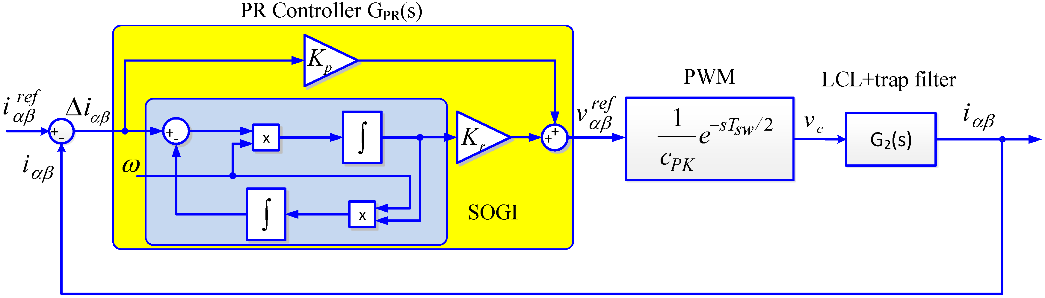
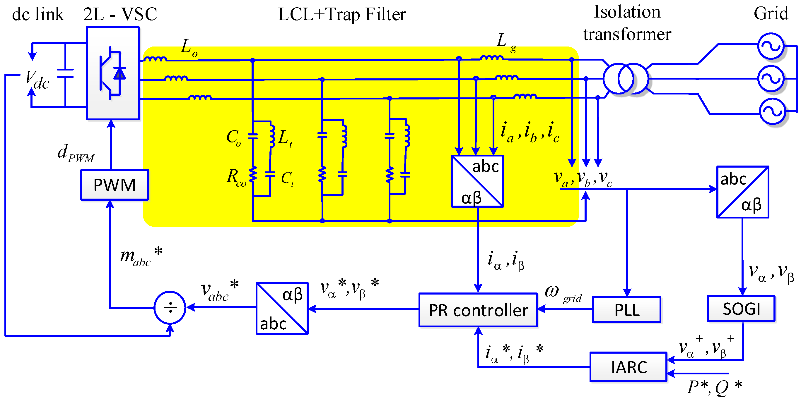
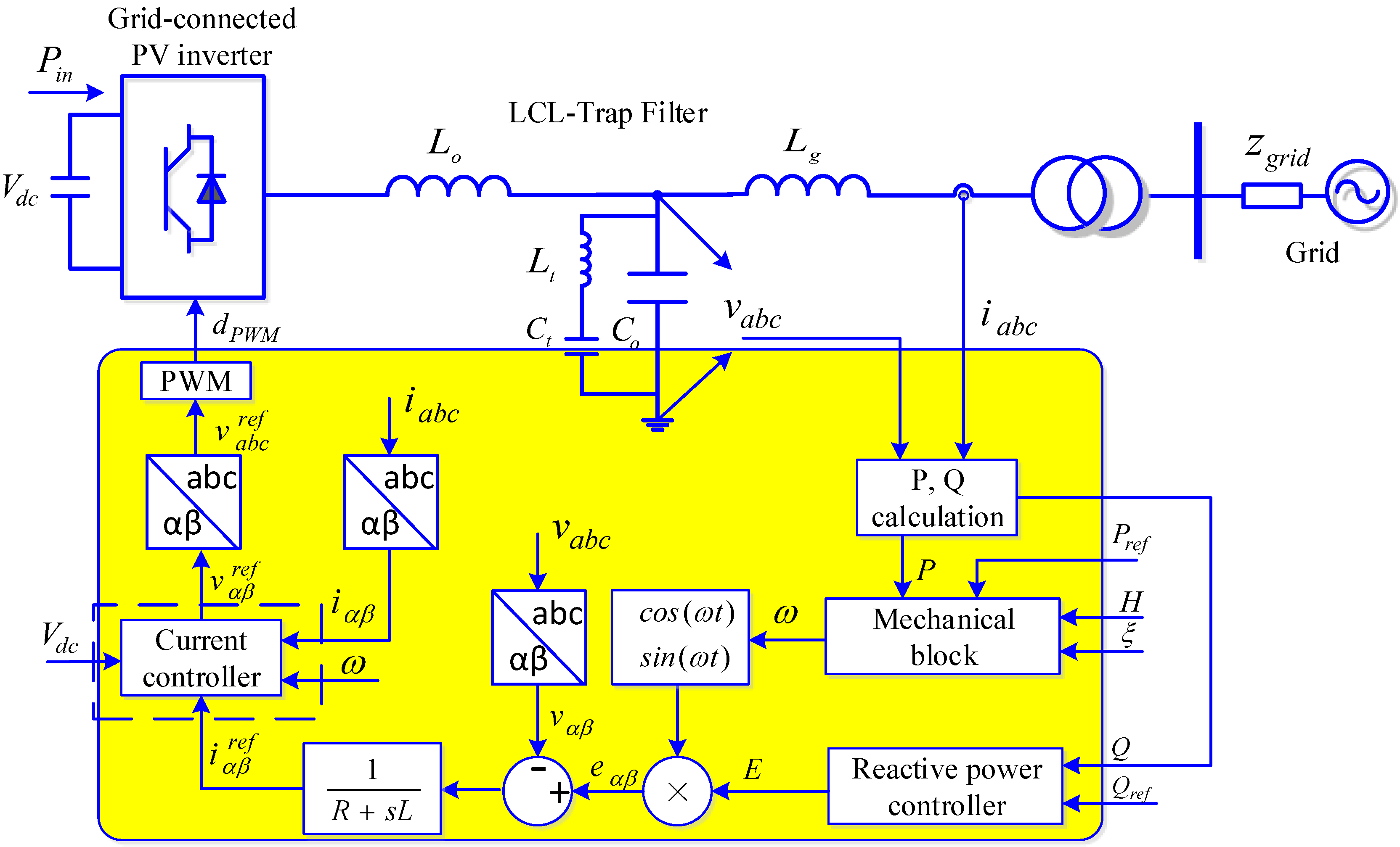
2. Proportional Resonant Controller for Grid-Connected Photovoltaic Inverters

Figure 1 shows the configuration of a PV generation plant that is connected to a 33-kV grid. It is comprised of 10 buses, and each one is supplied by two PV arrays through two paralleled grid-connected inverters.

The overall multi-loop control structure for each grid-connected converter of this plant is shown in Figure 2, which evolves from the general control framework of the synchronous power controller (SPC) that is proposed in [25]. The SPC stems from the concept of specifying the grid-connected converters with the electromechanical characteristics of synchronous machines and, hence, improves the interaction dynamics between the generation units and the grid. The reference of the current controller is provided by the virtual admittance block, which emulates the output impedance of synchronous machines. Inertia and damping characteristic can be given by configuring the mechanical block. Different strategies can be used for the control design of the mechanical block [26], and in this paper, a lead-lag structure is used [27]. The virtual synchronous frequency $\mathsf{\omega }$ is integrated with a phase angle $\mathsf{\theta }$, and combining the voltage magnitude $\mathit{E}$ generated by the reactive power controller, virtual electromotive force $\mathit{e}$ is generated.

As found from Figure 2, a fast and stable current controller is essential to achieve the designed functionalities that are specified by the SPC. In this paper, the stationary frame control paradigm is employed. The current regulating loop is modeled as Figure 3, where the current flowing through the grid-side inductor is adopted as the feedback variable.

The resonant part of the PR controller includes a second-order generalized integrator (SOGI) and a resonant gain $K_{\mathrm{r}}$, and $K_{\mathrm{p}}$ is the proportional gain. $T_{\mathrm{sw}}$ denotes the switching period, and due to the actual digital implementation that the duty signals are updated twice in each switching period, the computational delay is modeled to be half of the switching period. The gain of the PWM block is 1/$c_{\mathrm{PK}}$, where $c_{\mathrm{PK}}$ is the peak-to-peak value of the PWM triangular waveforms [22]. The LCL-trap filter [28,29] is employed as the grid connection filter, and $G_2\left(s\right)$ is the transfer function between the converter output voltage and grid-side current, which is expressed by Equation (1) in the continuous-time domain:

$$G_{\mathrm{f}}\left(s\right)={\displaystyle \frac{i_{\mathrm{g}}}{v}}\left(s\right)={\displaystyle \frac{C_{\mathrm{o}}{C}_{\mathrm{t}}{L}_{\mathrm{t}}{R}_{\mathrm{co}}{s}^3+C_{\mathrm{t}}{L}_{\mathrm{t}}{s}^2+C_{\mathrm{o}}{R}_{\mathrm{co}}s+1}{{\mathsf{\alpha }}_1{s}^5+{\mathsf{\alpha }}_2{s}^4+{\mathsf{\alpha }}_3{s}^3+{\mathsf{\alpha }}_4{s}^2+{\mathsf{\alpha }}_{5}s+{\mathsf{\alpha }}_6}}$$

(1)

where $L_{\mathrm{o}}$ and $L_{\mathrm{g}}$ are the converter-side inductance and grid-side inductance, respectively, $R_{\mathrm{o}}$ and $R_{\mathrm{g}}$ are the parasite equivalent resistance of the inductors $L_{\mathrm{o}}$ and $L_{\mathrm{g}}$, $C_{\mathrm{o}}$ is the filter capacitance, $R_{\mathrm{co}}$ is the passive damping resistance, and $C_{\mathrm{t}}$ and $L_{\mathrm{t}}$ are the capacitance and inductance of the trap branch, and the different coefficients in the denominator can be written as a function of the filter parameters shown as:

$$\begin{array}{c}{\mathsf{\alpha }}_1=C_{\mathrm{o}}{C}_{\mathrm{t}}{L}_{\mathrm{o}}{L}_{\mathrm{g}}{L}_{\mathrm{t}}\end{array}$$

(2)

$${\mathsf{\alpha }}_2=C_{\mathrm{o}}{C}_{\mathrm{t}}{L}_{\mathrm{o}}{L}_{\mathrm{g}}{R}_{\mathrm{co}}+C_{\mathrm{o}}{C}_{\mathrm{t}}{L}_{\mathrm{o}}{L}_{\mathrm{t}}{R}_{\mathrm{co}}+C_{\mathrm{o}}{C}_{\mathrm{t}}{L}_{\mathrm{g}}{L}_{\mathrm{t}}{R}_{\mathrm{co}}+C_{\mathrm{o}}{C}_{\mathrm{t}}{L}_{\mathrm{o}}{L}_{\mathrm{t}}{R}_{\mathrm{g}}+C_{\mathrm{o}}{C}_{\mathrm{t}}{L}_{\mathrm{g}}{L}_{\mathrm{t}}{R}_{\mathrm{o}}$$

(3)

$$\begin{array}{c}{\mathsf{\alpha }}_3=C_{\mathrm{o}}{L}_{\mathrm{o}}{L}_{\mathrm{g}}+C_{\mathrm{t}}{L}_{\mathrm{o}}{L}_{\mathrm{g}}+C_{\mathrm{t}}{L}_{\mathrm{o}}{L}_{\mathrm{t}}+C_{\mathrm{t}}{L}_{\mathrm{g}}{L}_{\mathrm{t}}+C_{\mathrm{o}}{C}_{\mathrm{t}}{L}_{\mathrm{o}}{R}_{\mathrm{g}}{R}_{\mathrm{co}}+C_{\mathrm{o}}{C}_{\mathrm{t}}{L}_{\mathrm{g}}{R}_{\mathrm{o}}{R}_{\mathrm{co}}\\ +C_{\mathrm{o}}{C}_{\mathrm{t}}{L}_{\mathrm{t}}{R}_{\mathrm{o}}{R}_{\mathrm{co}}+C_{\mathrm{o}}{C}_{\mathrm{t}}{L}_{\mathrm{t}}{R}_{\mathrm{co}}{R}_{\mathrm{g}}+C_{\mathrm{o}}{C}_{\mathrm{t}}{L}_{\mathrm{t}}{R}_{\mathrm{o}}{R}_{\mathrm{g}}\end{array}$$

(4)

$$\begin{array}{c}{\mathsf{\alpha }}_4=C_{\mathrm{o}}{L}_{\mathrm{o}}{R}_{\mathrm{co}}+C_{\mathrm{o}}{L}_{\mathrm{g}}{R}_{\mathrm{co}}+C_{\mathrm{o}}{L}_{\mathrm{o}}{R}_{\mathrm{g}}+C_{\mathrm{o}}{L}_{\mathrm{g}}{R}_{\mathrm{o}}+C_{\mathrm{t}}{L}_{\mathrm{o}}{R}_{\mathrm{g}}+C_{\mathrm{t}}{L}_{\mathrm{g}}{R}_{\mathrm{o}}+C_{\mathrm{t}}{L}_{\mathrm{t}}{R}_{\mathrm{o}}\\ +C_{\mathrm{t}}{L}_{\mathrm{t}}{R}_{\mathrm{g}}+C_{\mathrm{o}}{C}_{\mathrm{t}}{R}_{\mathrm{g}}{R}_{\mathrm{o}}{R}_{\mathrm{co}}\end{array}$$

(5)

$$\begin{array}{c}{\mathsf{\alpha }}_5=L_{\mathrm{o}}+L_{\mathrm{g}}+C_{\mathrm{o}}{R}_{\mathrm{co}}{R}_{\mathrm{o}}+C_{\mathrm{o}}{R}_{\mathrm{co}}{R}_{\mathrm{g}}+C_{\mathrm{o}}{R}_{\mathrm{o}}{R}_{\mathrm{g}}+R_{\mathrm{o}}{C}_{\mathrm{t}}{R}_{\mathrm{g}}\end{array}$$

(6)

$$\begin{array}{c}{\mathsf{\alpha }}_6=R_{\mathrm{o}}+R_{\mathrm{g}}\end{array}$$

(7)

As an alternative, if the converter-side current flowing through the inductor $L_{\mathrm{o}}$ is used as the controlled variable, the current control loop will have the same model, except that $G_2\left(s\right)$ should be substituted by $G_1\left(s\right)$ shown in Equation (8):

$${\displaystyle \frac{i_{\mathrm{c}}}{v}}\left(s\right)={\displaystyle \frac{1-G_{\mathrm{f}}\left(s\right)(L_{\mathrm{g}}s+R_{\mathrm{g}})}{L_{\mathrm{o}}s+R_{\mathrm{o}}}}$$

(8)

It has to be mentioned that the tuning procedure introduced in this paper is applicable to power converters with other types of filters, as long as the transfer function between the controlled current and converter output voltage can be extracted. Moreover, if the synchronous frame current control is adopted, the procedure will still be effective only by replacing the PR controller block in Figure 3 with the PI controller.

3. Unified Tuning Approach

A generalized current loop tuning procedure is proposed based on the modeling in the last section, and the stability and dynamic performance are analyzed based on numerical models.

3.1. Direct Discrete-Time Domain Design

Continuous-time derivations tend to work properly in digital implementations once the sampling rate is well above the controller bandwidth [30]. To overcome the limitations of the digital implementation in the case of lower switching frequency (thus, lower sampling frequency), in this paper, the control loop is modeled and tuned in the discrete-time domain. The transfer function of the PR controller in continuous-time domain $G_{\mathrm{PR}}\left(s\right)$ is shown in Equation (9):

$$G_{\mathrm{PR}}\left(s\right)=K_{\mathrm{P}}+K_{\mathrm{R}}·SOGI\left(s\right)=K_{\mathrm{P}}+K_{\mathrm{R}}·{\displaystyle \frac{{\mathsf{\omega }}_{0}s}{s^2+{\mathsf{\omega }}_0^2}}$$

(9)

The methods for discretizing the SOGI structure have been discussed in [31,32,33], and a thorough study is given in [31]. In this paper, the method proposed in [33] is used, where two integrators of the SOGI can be discretized separately. Employing the backward Euler method to discretize the integrator in the direct channel and the forward Euler method for the integrator in the feedback channel [33], the transfer function of the SOGI is discretized in the sampling period $T_{\mathrm{s}}$ and shown in Equation (10):

$$SOGI\left(z\right)={\displaystyle \frac{{\mathsf{\omega }}_0{T}_{\mathrm{s}}z(z-1)}{{(z-1)}^2+{\mathsf{\omega }}_0^2{T}_{\mathrm{s}}^{2}z}}$$

(10)

The transfer function of the plant $G_2\left(s\right)$ is discretized by the zero-order hold (ZOH) method. Since all of the values of the filter components are known, the discretization can be done using a computing language application. The open-loop transfer function in discrete-time domain $G_{\mathrm{OL}}\left(z\right)$ is then expressed in Equation (11):

$$G_{\mathrm{OL}}\left(z\right)={\displaystyle \frac{1}{c_{\mathrm{PK}}}}{G}_{\mathrm{PR}}\left(z\right)G_{\mathrm{f}}\left(z\right)$$

(11)

In Equation (11), $G_2\left(z\right)$ is the transfer function of the filter in the discrete-time domain. Since the ZOH transformation intrinsically introduces a delay corresponding to the PWM computational delay [9], the PWM delay has hence been included in the open-loop transfer function.

3.2. Calculation of the Controller Gains

The calculating algorithm based on the phase margin and crossover frequency is employed. According to the definitions, at crossover frequency ${\mathsf{\omega }}_{\mathrm{c}}$, the module of the open-loop transfer function is equal to one, and the phase angle is $-({180}^{\circ }-{\mathsf{\varphi }}_m)$, where ${\mathsf{\varphi }}_{\mathrm{m}}$ is the phase margin. In the continuous-time domain, this relation is shown in Equations (12) and (13):

$$|G_{\mathrm{OL}}\left(j{\mathsf{\omega }}_{\mathrm{c}}\right)|=1$$

(12)

$$\angle G_{\mathrm{OL}}\left(j{\mathsf{\omega }}_{\mathrm{c}}\right)=-({180}^{\circ }-{\mathsf{\varphi }}_{\mathrm{m}})$$

(13)

Examples on calculating the controller gains in the continuous-time domain with the crossover frequency and phase margin can be found in [9,22]. In this paper, based on the expressions in Section 3.1, the calculating is done in the discrete-time domain for easy digital implementation. In the discrete-time domain, the definitions of the phase margin and crossover frequency are shown in Equation (14):

$$G_{\mathrm{OL}}\left(e^{j{\mathsf{\omega }}_{\mathrm{c}}{T}_{\mathrm{s}}}\right)=1\angle -({180}^{\circ }-{\mathsf{\varphi }}_{\mathrm{m}})$$

(14)

Combining Equations (11) and (14) and assuming $c_{\mathrm{PK}}$ = 1, the below relation is obtained as shown in Equation (15):

$$G_{\mathrm{PR}}\left(e^{j{\mathsf{\omega }}_{\mathrm{c}}{T}_{\mathrm{s}}}\right)G_{\mathrm{f}}\left(e^{j{\mathsf{\omega }}_{\mathrm{c}}{T}_{\mathrm{s}}}\right)=1\angle -({180}^{\circ }-{\mathsf{\varphi }}_{\mathrm{m}})$$

(15)

As shown in Equation (15), the controller gains can be calculated once ${\mathsf{\omega }}_{\mathrm{c}}$ and ${\mathsf{\varphi }}_{\mathrm{m}}$ are fixed. In practice, the complex number in Equation (15) needs to be transformed into two real number equations by extracting the real part and imaginary part, respectively, as shown in Equations (16) and (17):

$$Re\left\{G_{\mathrm{PR}}\left(e^{j{\mathsf{\omega }}_{\mathrm{c}}{T}_{\mathrm{s}}}\right)G_{\mathrm{f}}\left(e^{j{\mathsf{\omega }}_{\mathrm{c}}{T}_{\mathrm{s}}}\right)\right\}=Re\left\{1\angle -({180}^{\circ }-{\mathsf{\varphi }}_{\mathrm{m}})\right\}$$

(16)

$$Im\left\{G_{\mathrm{PR}}\left(e^{j{\mathsf{\omega }}_{\mathrm{c}}{T}_{\mathrm{s}}}\right)G_{\mathrm{f}}\left(e^{j{\mathsf{\omega }}_{\mathrm{c}}{T}_{\mathrm{s}}}\right)\right\}=Im\left\{1\angle -({180}^{\circ }-{\mathsf{\varphi }}_{\mathrm{m}})\right\}$$

(17)

If $z_{\mathrm{c}}$ is defined to be the value of z when $\mathsf{\omega }$ is fixed to ${\mathsf{\omega }}_{\mathrm{c}}$, then Equations (16) and (17) can be transformed into Equation (18):

$$\left[K_{\mathrm{P}}{K}_{\mathrm{R}}\right]\left[\begin{array}{cc}1& 0\\ Re\left\{SOGI\left(z_{\mathrm{c}}\right)\right\}& Im\left\{SOGI\left(z_{\mathrm{c}}\right)\right\}\end{array}\right]=\left[Re\left(a\right)Im\left(a\right)\right]$$

(18)

where the constant a is expressed in Equation (19):

$$a={\displaystyle \frac{1\angle -({180}^{\circ }-{\mathsf{\varphi }}_{\mathrm{m}})}{G_{\mathrm{f}}\left(e^{j{\mathsf{\omega }}_{\mathrm{c}}{T}_{\mathrm{s}}}\right)}}$$

(19)

It is worth noting that by using a typical computing language application, Equation (18) can be easily expressed and processed.

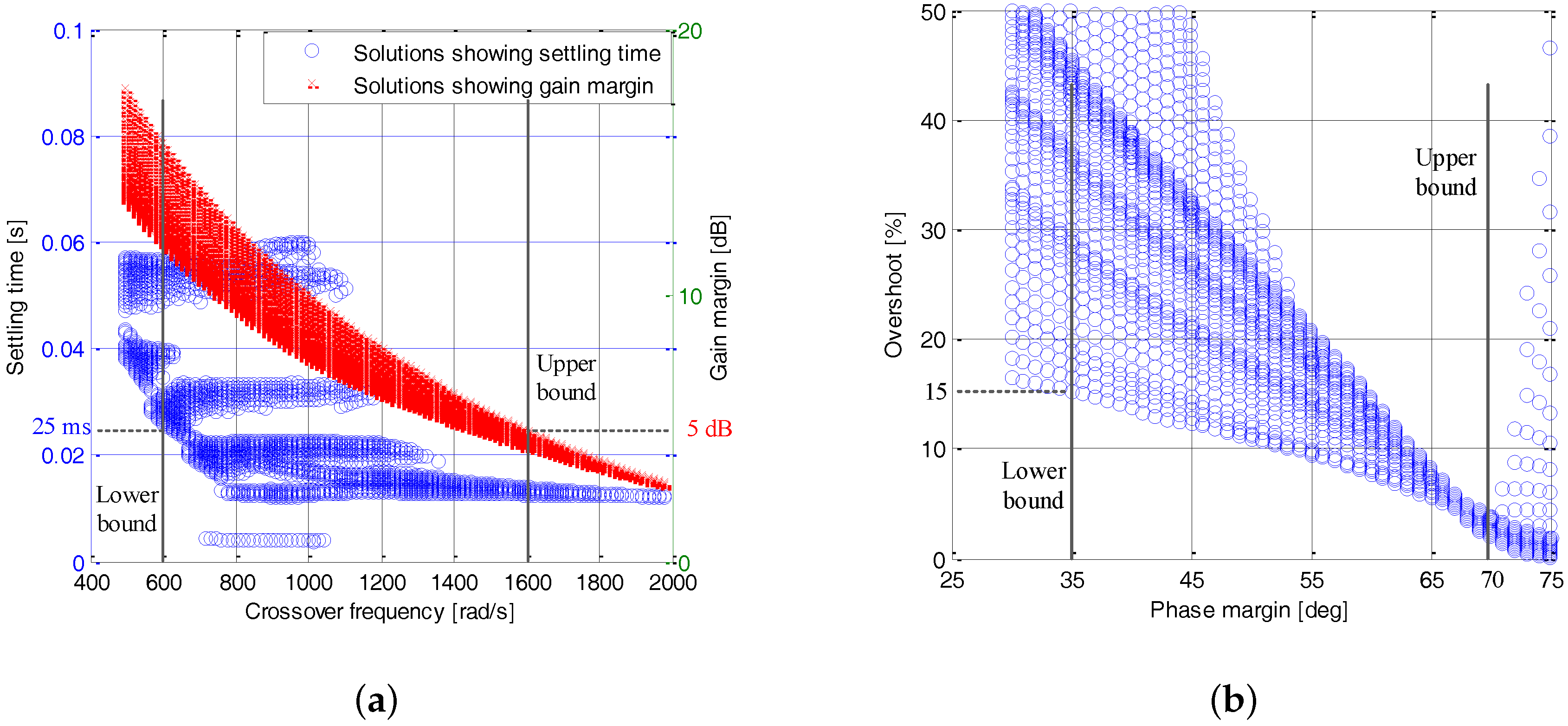
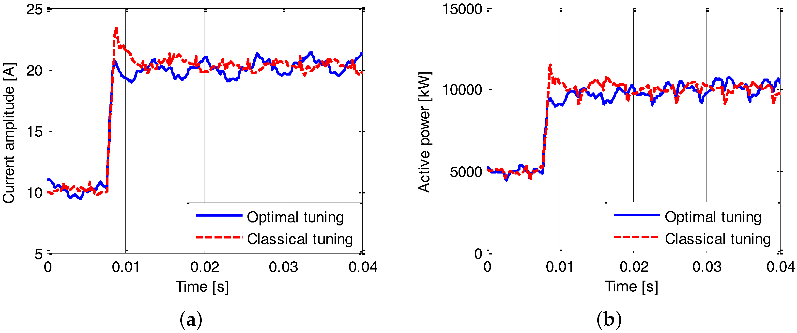
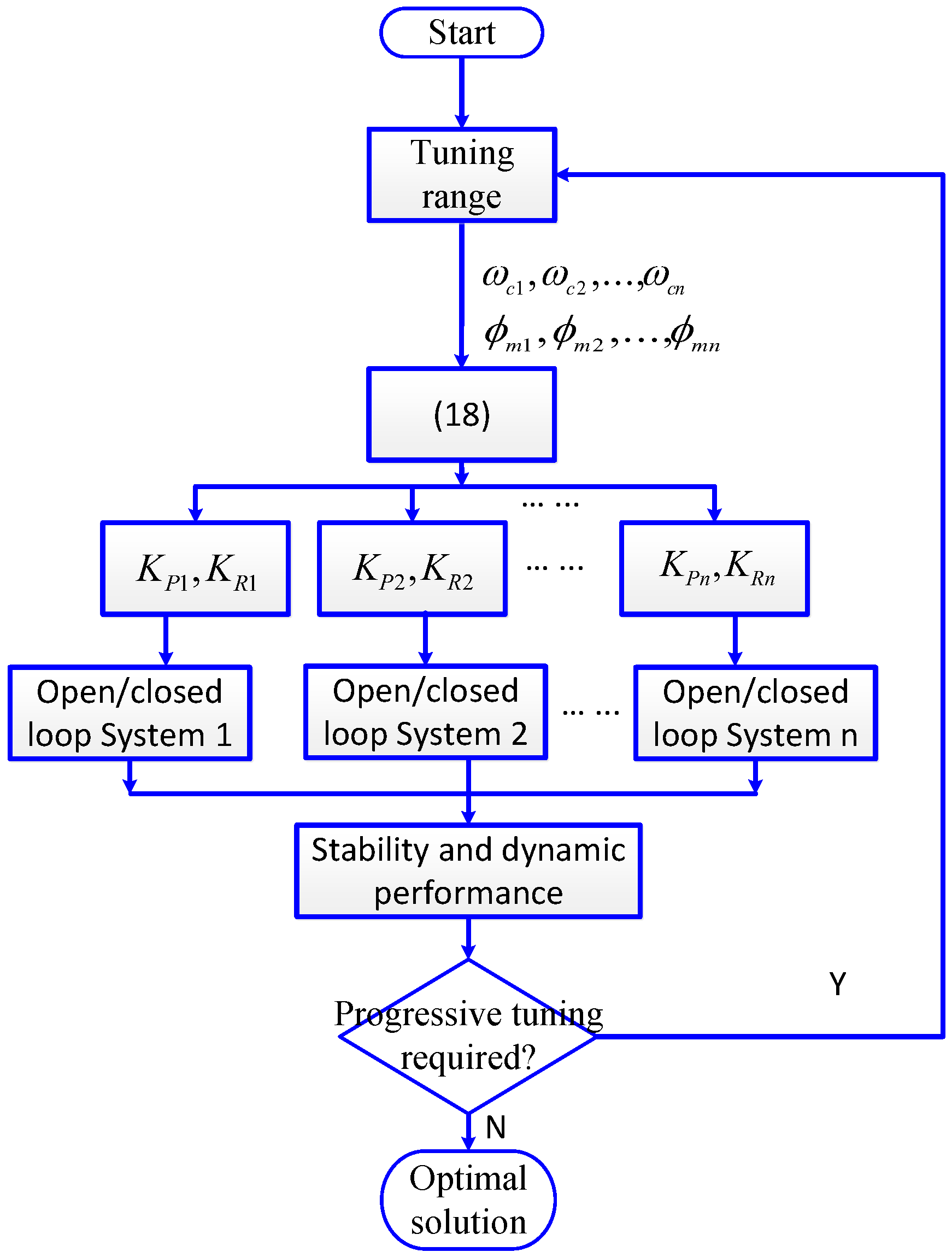
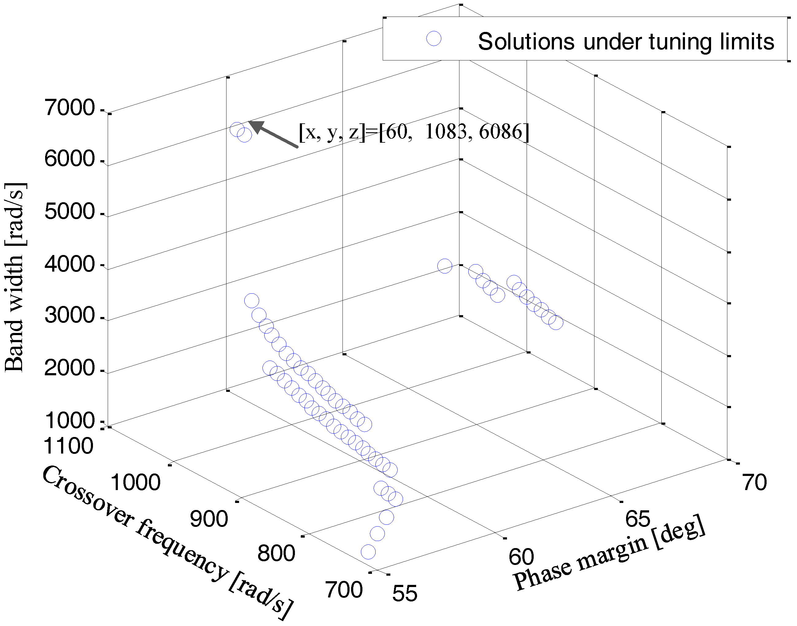
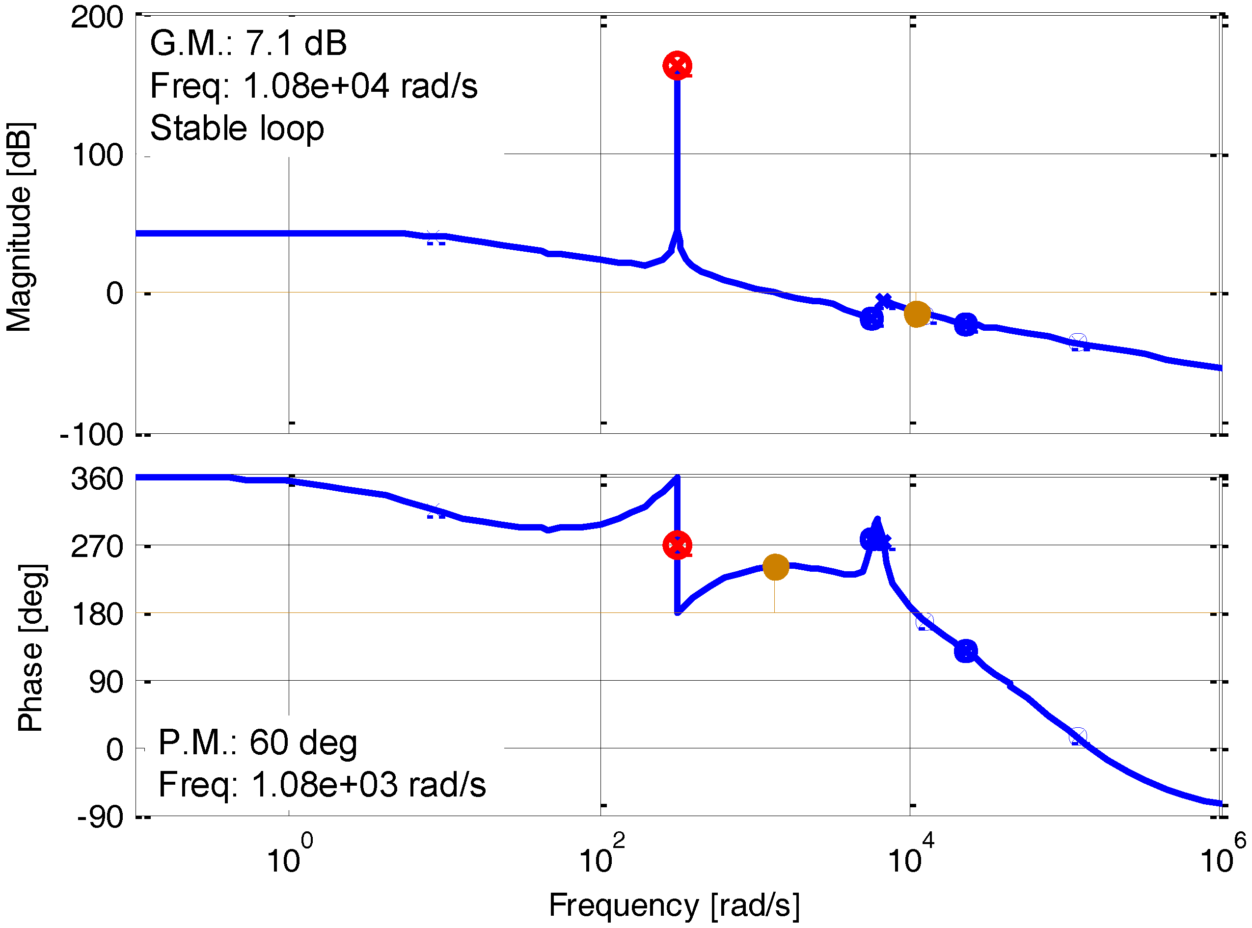
3.3. Optimized Tuning

The controller gains $K_{\mathrm{p}}$ and $K_{\mathrm{r}}$ can be calculated by solving Equation (18), which acts as a calculator; however, giving appropriate inputs for ${\mathsf{\omega }}_{\mathrm{c}}$ and ${\mathsf{\varphi }}_{\mathrm{m}}$ needs further analysis.

For a second-order closed-loop system, the gains can be determined by specifying the damping coefficient and the step response settling time, as shown in [33]. However, for a high order system, a straightforward relation between the dynamics and the controller gains is hard to find. A usual approach is to make a reasonable approximation for the open-loop transfer function [9,22], or particularly, approximating the model of grid-connection filter [11,34,35]. However, justifications of the approximation have to be given, as well as the boundaries of application. In order to provide a general tuning procedure instead of an application-specific one, the closed-loop systems defined by different sets of controller gains are evaluated and compared with each other analytically in the proposed approach in terms of stability and dynamics. The procedures of the tuning are summarized in Figure 4.

In the first step, ${\mathsf{\omega }}_{\mathrm{c}}$ and ${\mathsf{\varphi }}_{\mathrm{m}}$ are specified with numerous values within the initial tuning range, respectively, and for each set of ${\mathsf{\omega }}_{\mathrm{c}}$ and ${\mathsf{\varphi }}_{\mathrm{m}}$, a set of $K_{\mathrm{p}}$ and $K_{\mathrm{r}}$ will be obtained through Equation (18). Commonly, the phase margin reflects the stability, and the crossover frequency reflects the bandwidth. Therefore, it is easy to designate an initial tuning range in advance. Then, different sets of controller gains will be obtained, and each set will lead to an open-loop and a closed-loop system. By the assessment of the open-loop stability margin, the closed-loop unitary step response and closed-loop bandwidth, each solution is evaluated, and an updated tuning range is determined for progressive tuning.

In the tuning procedure, even though the phase margin has been specified for calculating the controller gains, it has to be checked again after the controller gains are calculated. As mentioned in [11], in some scenarios when the PR controller is assigned to track harmonics, additional open-loop resonant poles will occur, resulting in the practical phase margin being lower than the specification.

When the tuning range is updated in the first step, another round of tuning is activated with a smaller interval for the inputs. In this manner, progressive tuning is executed until an optimized solution is found.

A 100-kW three-phase two-level grid-connected converter with the LCL-trap filter is used to elaborate the tuning method. The associated parameters of the plant are shown in

Table 1. Parameters of the 100-kW converter.

Parameter	Value	Parameter	Value
$V_{\mathrm{dc}}$ (V)	750	$R_{\mathrm{g}}$ (Ω)	0.0021
$L_{\mathrm{o}}$ ($\mathsf{\mu }$H)	778	$R_{\mathrm{co}}$ (Ω)	0.5
$L_{\mathrm{g}}$ ($\mathsf{\mu }$H)	402	$S_{\mathrm{N}}$ (kW)	100
$C_{\mathrm{o}}$ ($\mathsf{\mu }$F)	66	$f_{\mathrm{sw}}$ (Hz)	3150
$C_{\mathrm{t}}$ ($\mathsf{\mu }$F)	30	$f_{\mathrm{s}}$ (Hz)	6300
$L_{\mathrm{t}}$ ($\mathsf{\mu }$H)	85	$U_{\mathrm{g}}$ (V)	400
$R_{\mathrm{o}}$ (Ω)	0.0073	$f_{\mathrm{g}}$ (Hz)	50

. Then, the transfer function of the plant in the discrete time domain is obtained as Equation (20).

$$G_{\mathrm{f}}\left(z\right)={\displaystyle \frac{0.032z^4+0.091z^3+0.090z^2+0.035z+0.004}{z^5-1.126z^4+0.384z^3+0.201z^2-0.167z-0.291}}$$

(20)

The tuning boundaries in this case are shown in

Table 2. Tuning boundaries of the current controller.

Variable	Symbol	Boundary
Settling time (ms)	$t_{\mathrm{ss}}$	<25
Overshoot (%)	$o_{\mathrm{s}}$	<15
Gain margin (dB)	$G_{\mathrm{m}}$	>5
Phase margin (degree)	${\mathsf{\varphi }}_{\mathrm{m}}$	>35

, where settling time and overshoot are the ones calculated based on the closed-loop unitary step response. These requirements are used as the criteria to eliminate the ineligible solutions in the tuning.

Figure 5 is plotted by specifying different values for ${\mathsf{\omega }}_{\mathrm{c}}$ and ${\mathsf{\varphi }}_{\mathrm{m}}$ in a large range, and for each obtained solution of $K_{\mathrm{p}}$ and $K_{\mathrm{r}}$, the open-loop stability margin, settling time $t_{\mathrm{ss}}$ and overshoot of the closed-loop unitary step response and the closed-loop bandwidth are calculated. Figure 5a,b, respectively, shows the influence of ${\mathsf{\omega }}_{\mathrm{c}}$ and ${\mathsf{\varphi }}_{\mathrm{m}}$ on the performance of the system.

In Figure 5a, the influence of the crossover frequency on the settling time $t_{\mathrm{ss}}$ and the gain margin are both shown. Both relations have a visible trend. When ${\mathsf{\omega }}_{\mathrm{c}}$ increases from 500 rad to 800 rad, $t_{\mathrm{ss}}$ has a general trend of reducing, while the gain margin has a general trend of reducing in the full range of ${\mathsf{\omega }}_{\mathrm{c}}$. Figure 5a also visualizes the tradeoff between the system stability and dynamics and shows that ${\mathsf{\omega }}_{\mathrm{c}}$ with a value either too big or too small shall not be adopted. When ${\mathsf{\omega }}_{\mathrm{c}}$ is above 1600 rad, the gain margin is smaller than 5 dB. In order to ensure the stability of the system, solutions with a gain margin smaller than 5 dB are not accepted in the tuning. Therefore, the upper bound of ${\mathsf{\omega }}_{\mathrm{c}}$ is selected to be 1600 rad. Additionally, when ${\mathsf{\omega }}_{\mathrm{c}}$ is below 600 rad, $t_{\mathrm{ss}}$ is greater than 25 ms. In order to ensure the speed of response, solutions with $t_{\mathrm{ss}}$ greater than 25 ms are not accepted in the tuning. Therefore, the lower bound ${\mathsf{\omega }}_{\mathrm{c}}$ is selected to be 600 rad. Therefore, the updated input range of ${\mathsf{\omega }}_{\mathrm{c}}$ is obtained and shown in Equation (21), where $d\mathsf{\omega }$ is the interval of the inputs, which is selected to be 10 rad.

$${\mathsf{\omega }}_{\mathrm{c}}=\{600,600+d\mathsf{\omega },600+2d\mathsf{\omega },\dots ,1600\}$$

(21)

Figure 5b shows the relation between overshoot and ${\mathsf{\varphi }}_{\mathrm{m}}$. When ${\mathsf{\varphi }}_{\mathrm{m}}$ increases, the overshoot generally reduces. When ${\mathsf{\varphi }}_{\mathrm{m}}$ is smaller than ${35}^{\circ }$, there is not a solution with an overshoot lower than 15%. Since responses with a large overshoot could render the converters to be oversized, the lower bound of ${\mathsf{\varphi }}_{\mathrm{m}}$ is selected to be ${35}^{\circ }$. Additionally, the upper bound is selected to be ${70}^{\circ }$. The updated tuning range of ${\mathsf{\varphi }}_m$ is obtained and shown in Equation (22):

$${\mathsf{\varphi }}_{\mathrm{m}}=\{{35}^{\circ },{36}^{\circ },{37}^{\circ },...,{70}^{\circ }\}$$

(22)

Even though some solutions that do not meet the tuning requirements have been eliminated once the tuning range shown in Equations (21) and (22) is obtained, the tuning limits shown in Table 2 are still necessary in the further tuning process to eliminate all of the undesired solutions. With the inputs shown in Equations (21) and (22), different sets of $K_p$ and $K_r$ are obtained. All of the solutions that lead to a performance within the limits will be seen as eligible and stored, and one optimal solution can further be selected.

Figure 6 shows the bandwidth of the closed-loop systems in relation with ${\mathsf{\omega }}_c$ and ${\mathsf{\varphi }}_m$ based on the eligible solutions. The solution with the largest bandwidth is selected as the optimal one, which is shown in

Table 3. Selected solution of the controller gains.

Parameter	Symbol	Value
Proportional gain	$K_{\mathrm{p}}$	1.2192
Resonant gain	$K_{\mathrm{r}}$	0.5593
Settling time (ms)	$t_{\mathrm{ss}}$	22.5
Overshoot (%)	$o_{\mathrm{s}}$	14.66
Gain margin (dB)	$G_{\mathrm{m}}$	7.1276
Phase margin (degree)	${\mathsf{\varphi }}_{\mathrm{m}}$	60
Band width (rad/s)	$B_{\mathrm{w}}$	6086
Crossover frequency (rad/s)	${\mathsf{\omega }}_{\mathrm{c}}$	1083

. It is shown in Figure 6 that the eligible solutions mostly gather in the range of ${\mathsf{\omega }}_{\mathrm{c}}$ = [900 rad, 1100 rad] and ${\mathsf{\varphi }}_{\mathrm{m}}=[{55}^{\circ },{70}^{\circ }]$. It is worth mentioning that the number of eligible solutions can be increased simply by reducing the input interval $d\mathsf{\omega }$.

Based on the selected optimal solution, the Bode plot of the open-loop system is shown in Figure 7, where the stability is validated. By applying the above tuning procedure, the phase margin and crossover frequency can be determined in a reasonable manner according to the specified stability and dynamics limits.

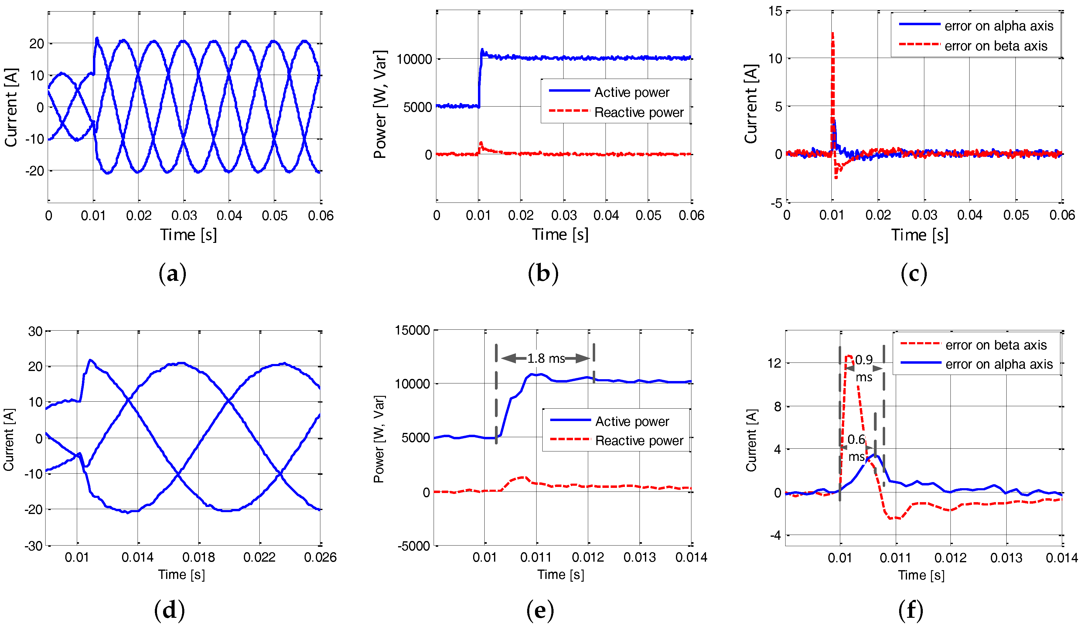
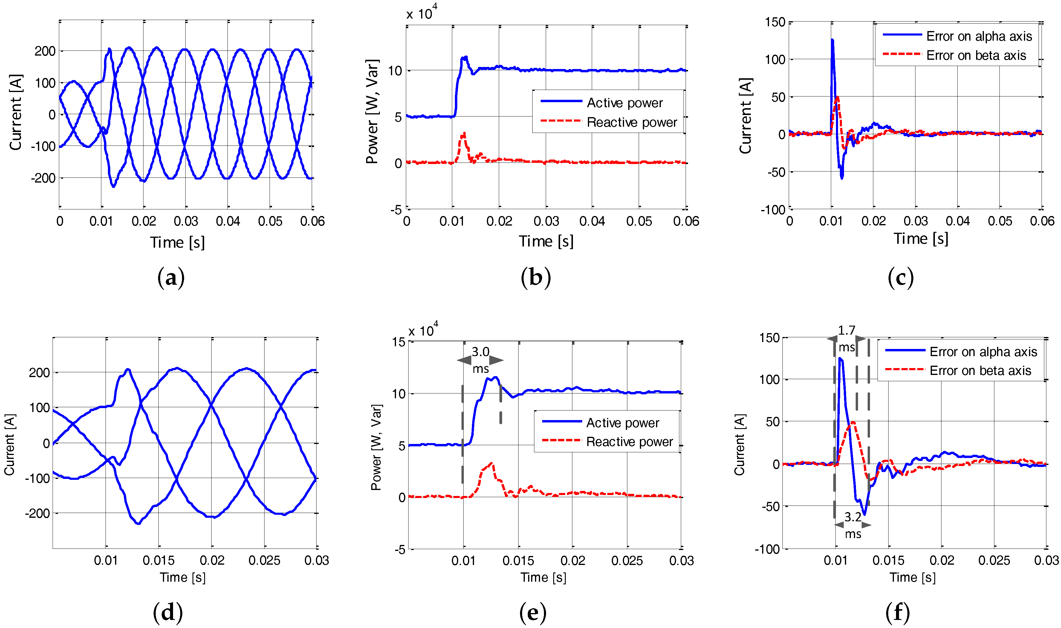
4. Simulation Results

The current loop tuning method is validated in simulations in this section. Simulated plants of 10-kW and 100-kW power ratings are used respectively in two cases, and the response of the current loop in the presence of reference changes is evaluated. For simplicity in the primary validation, a simple outer loop control strategy is used, as shown in Figure 8, instead of using the multi-loop control structure, shown in Figure 2. With the aid of the stationary-frame phase-locked loop (PLL) [36], the frequency of the grid ${\mathsf{\omega }}_{\mathrm{grid}}$ is estimated based on the measurement of three-phase grid voltage. The references of the current controller $i_{\mathsf{\alpha }}^{*}$ and $i_{\mathsf{\beta }}^{*}$ are provided according to the instantaneous active reactive controller (IARC) [37] shown in Equations (23) and (24).

$$i_{\mathsf{\alpha }}^{*}={\displaystyle \frac{P{v}_{\mathsf{\alpha }}^{+}+Q{v}_{\mathsf{\beta }}^{+}}{v_{\mathsf{\alpha }}^{+2}+v_{\mathsf{\beta }}^{+2}}}$$

(23)

$$i_{\mathsf{\beta }}^{*}={\displaystyle \frac{P{v}_{\mathsf{\beta }}^{+}-Q{v}_{\mathsf{\alpha }}^{+}}{v_{\mathsf{\alpha }}^{+2}+v_{\mathsf{\beta }}^{+2}}}$$

(24)

where $P^{*}$ and $Q^{*}$ are the reference of active and reactive power and $v_{\mathsf{\alpha }}^{+}$ and $v_{\mathsf{\beta }}^{+}$ the positive sequence components of grid voltage in the stationary frame filtered by a double SOGI.

The parameters of the 10-kW converter and the controller are shown in

Table 4. Parameters of the 10-kW converter and the selected controller gains.

Parameter	Value	Parameter	Value
$V_{\mathrm{dc}}$ (V)	640	$R_{\mathrm{g}}$ (Ω)	0.094
$L_{\mathrm{o}}$ (mH)	2.6	$R_{\mathrm{co}}$ (Ω)	1
$L_{\mathrm{g}}$ ($\mathsf{\mu }$H)	662	$S_{\mathrm{N}}$ (kW)	10
$C_{\mathrm{o}}$ ($\mathsf{\mu }$F)	5.5	$f_{\mathrm{sw}}$ (Hz)	10,050
$C_{\mathrm{t}}$ ($\mathsf{\mu }$F)	1	$f_{\mathrm{s}}$ (Hz)	10,050
$L_{\mathrm{t}}$ ($\mathsf{\mu }$H)	244	$U_{\mathrm{g}}$ (V)	400
$R_{\mathrm{o}}$ (Ω)	0.025	$f_{\mathrm{g}}$ (Hz)	50
$K_{\mathrm{p}}$	8.7818	$K_{\mathrm{r}}$	7.7968

. The simulation results of the 10-kW system are shown in Figure 9, where the steady-state and dynamic performances are shown. A power reference of 5 kW and 0 kVar is given initially, and it changes to 10 kW and 0 kVar at 0.01 s.

Figure 9a shows the waveforms of three-phase current, and it is regulated properly in both steady-state and transient without oscillations. Figure 9b shows the profiles of instantaneous power injected by the converter. The settling time of the experimental transient response is calculated by Equation (25), where $I\left(s\right)$ is the experimental data vector (that will be the active power response or current control error response in the following cases), $I_{\mathrm{ss}}$ is the value of the last element in the data vector and ${\mathsf{\epsilon }}_{\mathrm{ss}}$ is the specified steady-state band:

$$t_{\mathrm{s}}=\min \{ts.t.\mid {\displaystyle \frac{I\left(s\right)}{I_{\mathrm{ss}}}}-1\mid <{\mathsf{\epsilon }}_{\mathrm{ss}}\forall s>t\}$$

(25)

If 5% of the nominal power is defined as the steady-state band, then the active power regulation settling time is calculated to be 1.8 ms. Figure 9c shows the tracking performance of the current controller on the $\mathsf{\alpha }$ and $\mathsf{\beta }$ axis. If 10% of the magnitude of the nominal current is defined as the steady-state band, then the settling times of the current controller on the $\mathsf{\alpha }$ and $\mathsf{\beta }$ axis are, respectively, 0.9 ms and 0.6 ms. A fast response of the current loop is demonstrated.

The parameters of the 100-kW setups and the controller are shown in Table 1 and Table 3. Additionally, the simulation results of the 100-kW system are shown in Figure 10, where a step change of the active power reference from 50 kW to 100 kW is given at 0.01 s.

Figure 10a shows the waveforms of three-phase current. In addition to the case of 10-kW system, the grid injected current is regulated properly in the steady-state and presents a fast transient response. Figure 10b shows the instantaneous power injection. If 5% of the nominal power is defined as the steady-state band, the active power regulation settling time is calculated to be 3.0 ms. Figure 10c shows the tracking performance of the current controller on the $\mathsf{\alpha }$ and $\mathsf{\beta }$ axis. If 10% of the magnitude of the nominal current is defined as the steady-state band, the settling times of the current controller on the $\mathsf{\alpha }$ and $\mathsf{\beta }$ axis are 3.2 ms and 1.7 ms, respectively.

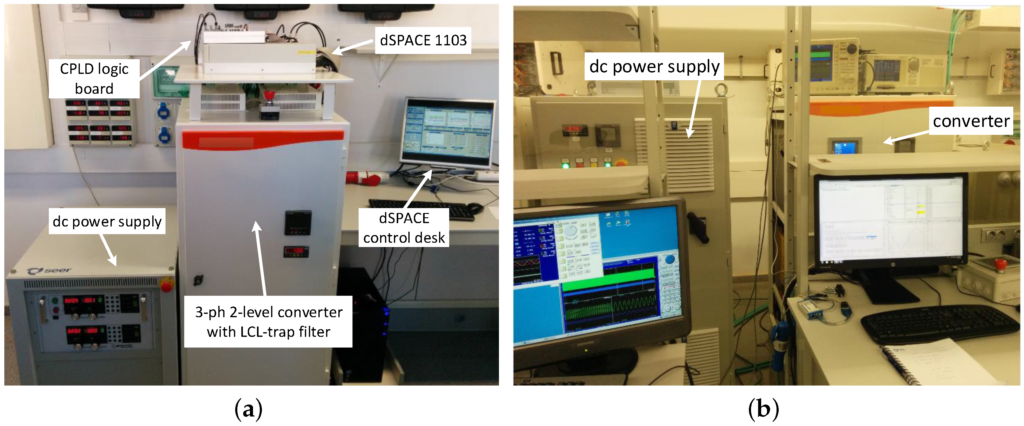
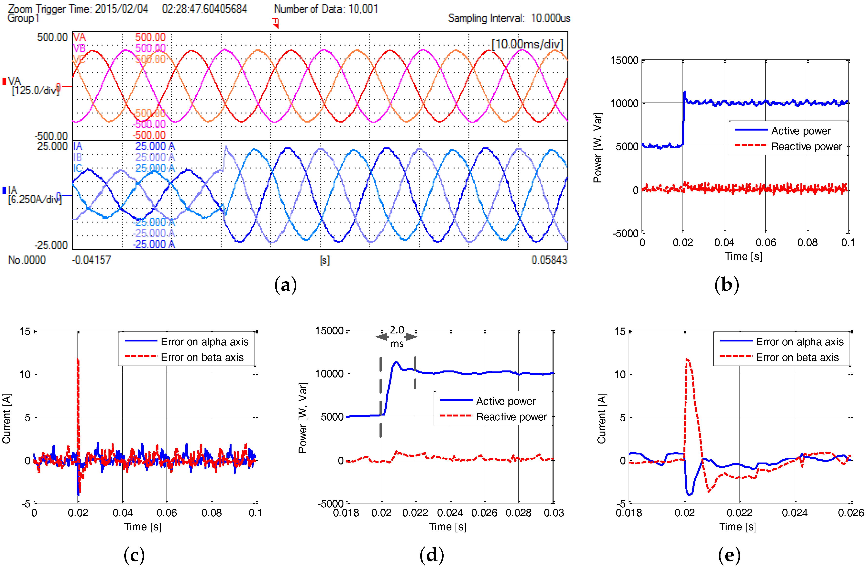
5. Experimental Results

Experimental tests are conducted on 10-kW and 100-kW laboratory test beds in order to further validate the proposed tuning method. The parameters of the setups are the ones shown in Table 1 and Table 4. The setups of the 10-kW system are shown in Figure 11a, and the setups of the 100-kW system are shown in Figure 11b.

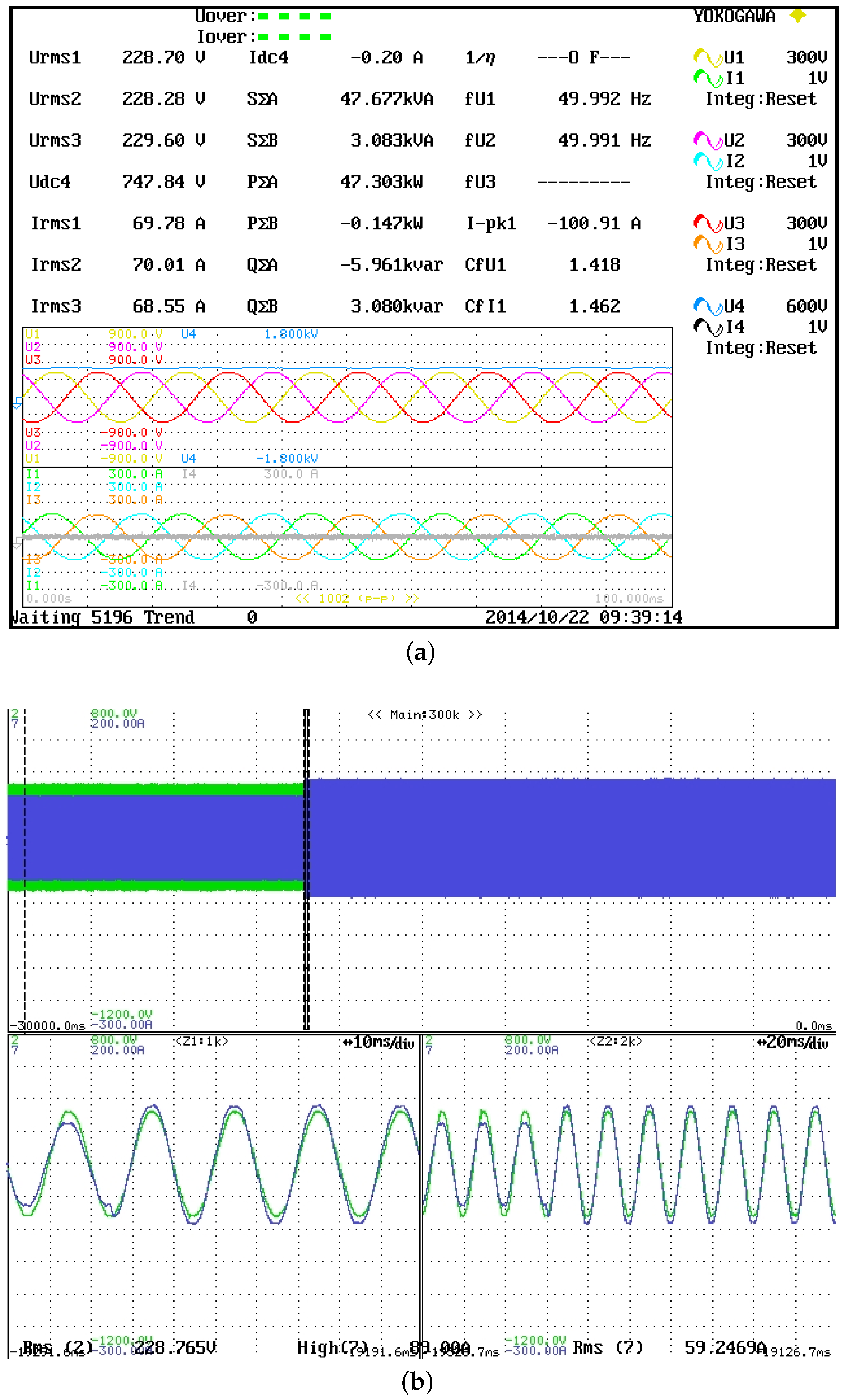
5.1. Steady-State and Dynamic Performance

Firstly, the performance of the current loop in the presence of reference changes is evaluated with the simple outer loop control strategy that is used in the simulations. The current loop steady-state and dynamic performance based on the 10-kW system are shown in Figure 12. Figure 12a shows the grid voltage and injected current, where the current is regulated with a fast response as in the simulation. Figure 12b shows the instantaneous active and reactive power injected into the grid. With the same definition of the steady-state band as the simulation (5%), the settling time of the active power is calculated to be 2.0 ms. Additionally, the current regulating errors on the $\mathsf{\alpha }$ and $\mathsf{\beta }$ axis (recorded data in dSPACE) are shown in Figure 12c. The above experimental results have demonstrated the fast dynamics of the current loop, like the ones in the simulation results.

The current loop steady-state and dynamic performances based on the 100-kW system are shown in Figure 13. Figure 13a is captured when the set point of the power is 50 kW and 0 kVar, and the good steady-state performance of the controller is shown. The transient responses of the current controller are shown in Figure 13b, when the active power reference jumps from 35 kW to 50 kW. The current is shown to be regulated quickly without a big overshoot.

Further, the proposed tuning method is compared with a classical tuning method that is proposed in [9]. According to the proposed optimal tuning, numerous inputs of the crossover frequency and phase margin are given to calculate the controller gains. The tuning limits are the same as Table 2, except that the overshoot is limited to 5%. Among all of the eligible solutions, the one that has the greatest bandwidth is selected. In comparison, according to the method in [9], the phase margin is fixed to ${40}^{\circ }$, and the crossover frequency is fixed using Equation (26), where $T_{\mathrm{d}}$ is the modeling of the delay in the loop:

$${\mathsf{\omega }}_{\mathrm{c}}=\frac{\mathsf{\pi }/2-{\mathsf{\varphi }}_{\mathrm{m}}}{T_{\mathrm{d}}}$$

(26)

The tests are conducted in the 10-kW platform. It is shown in Figure 14 that the transient response of the current control based on optimal tuning has a similar speed compared to the classical tuning, but has a smaller overshoot thanks to the tuning limit of the overshoot.

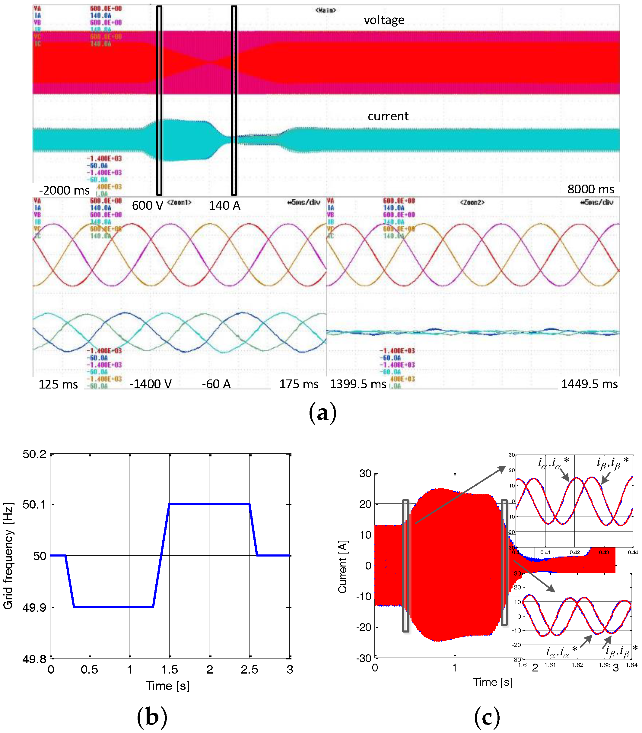
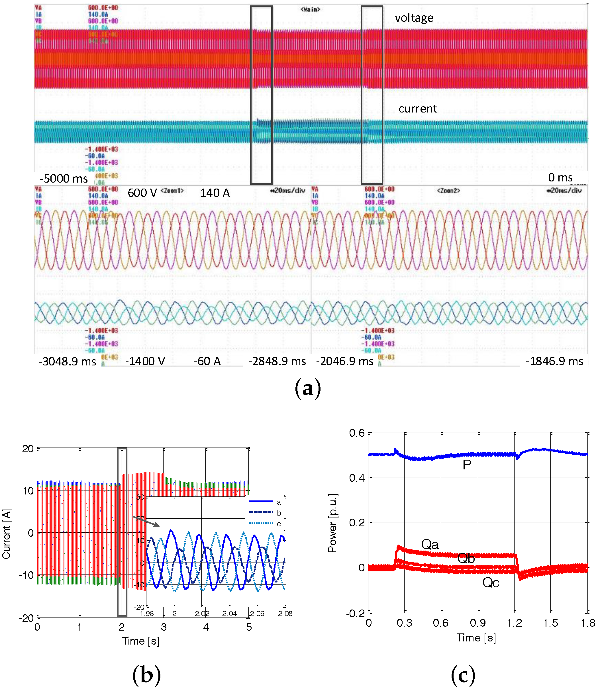
5.2. Performance under Grid Voltage and Frequency Changes

Further, the current controller is implemented in the overall SPC control scheme shown in Figure 2 to evaluate its performance in the presence of voltage and frequency changes in the grid. The 10-kW setups are used to implement the controller.

In the first scenario, grid frequency variations are given by configuring a regenerative AC power source, California Instruments MX-45 (Ametek, San Diego, CA, USA). Because of the low output impedance of the regenerative power source, the grid voltage waveforms are independent of the power injection of the converter. In this way, the response of the converter related to grid frequency can be clearly shown.

The frequency variation of the grid is specified as shown in Figure 15b; the frequency changing slope is ±1 Hz/s. It can be seen in Figure 15a that the current is well regulated; meanwhile, the power injection of the converter opposes the frequency deviation of the grid thanks to the inertia and droop characteristics of the SPC. In order to clearly show the inertia effect, the inertia constant is specified to be 10 s. Particularly, the tracking performance of the tuned current controller is shown in Figure 15c, where the controlled current tracks its reference without visible steady-state error or delay.

In the second scenario, unbalanced voltage sag is given, and the results are shown in Figure 16. The sag of one phase is generated and lasts 1 s, and the phase-to-neutral voltage rms is reduced from 230 V to 190 V. During the sag, the converter keeps connected to the grid, and the injected current is seen to be stable without significant oscillations in Figure 16a,b. As shown in Figure 16c, the injected reactive power in the sag phase presents a significant voltage supporting behavior thanks to the virtual admittance characteristics of the SPC, while the injected reactive power in the other two phases does not experience significant variations. The virtual admittance is achieved based on the well-tuned inner current loop.

6. Conclusions

A unified current loop tuning procedure was proposed in this paper as a general approach for the control design of grid-connected PV inverters. An analysis-based method was used to determine the system crossover frequency and phase margin, instead of the experience-based method that is seen in existing studies. Additionally, a direct discrete-time domain tuning was used based on the discretized modeling of the system, which guarantees the effectiveness of the controller in digital implementation. Finally, the tuning results were validated in simulation and experiments in different scenarios, where the current loop presents a fast transient response and good steady-state performance. With a good foundation in the current loop, the converter exhibited grid-supporting characteristics when the outer loops of the SPC were activated.

References

1. Van Wesenbeeck, M.P.N.; de Haan, S.W.H.; Varela, P.; Visscher, K. Grid tied converter with virtual kinetic storage. In Proceedings of the 2009 IEEE Bucharest PowerTech, Bucharest, Romania, 28 June–2 July 2009; pp. 1–7.
2. Alatrash, H.; Mensah, A.; Mark, E.; Haddad, G.; Enslin, J. Generator emulation controls for photovoltaic inverters. IEEE Trans. Smart Grid 2012, 3, 996–1011. [Google Scholar] [CrossRef]
3. Lai, N.B.; Kim, K.-H. An Improved Current Control Strategy for a Grid-Connected Inverter under Distorted Grid Conditions. Energies 2016, 9, 190. [Google Scholar] [CrossRef]
4. Hirase, Y.; Abe, K.; Sugimoto, K.; Shindo, Y. A grid-connected inverter with virtual synchronous generator model of algebraic type. Electr. Eng. Jpn. 2013, 184, 10–21. [Google Scholar] [CrossRef]
5. Rodriguez, P.; Candela, I.; Luna, A. Control of PV Generation Systems Using the Synchronous Power Controller. In Proceedings of the 2013 IEEE Energy Conversion Congress and Exposition (ECCE), Denver, CO, USA, 15–19 September 2003; pp. 993–998.
6. Nanou, S.I.; Papakonstantinou, A.G.; Papathanassiou, S.A. A generic model of two-stage grid-connected PV systems with primary frequency response and inertia emulation. Electr. Power Syst. Res. 2015, 127, 186–196. [Google Scholar] [CrossRef]
7. Network Code for Requirements for Grid Connection Applicable to all Generators; European Network of Transmission System Operators for Electricity (ENTSO-E): Brussels, Belgium, 2012.
8. Nationalgrid. The Grid Code Issue 5 Revision 7; Nationalgrid: London, UK, 2010. [Google Scholar]
9. Holmes, D.G.; Lipo, T.A.; McGrath, B.P.; Kong, W.Y. Optimized design of stationary frame three phase AC Current regulators. IEEE Trans. Power Electron. 2009, 24, 2417–2426. [Google Scholar] [CrossRef]
10. Yuan, X.; Merk, W.; Stemmler, H.; Allmeling, J. Stationary-frame generalized integrators for current control of active power filters with zero steady-state error for current harmonics of concern under unbalanced and distorted operating conditions. IEEE Trans. Ind. Appl. 2002, 38, 523–532. [Google Scholar] [CrossRef]
11. Yepes, A.G.; Freijedo, F.D.; Lopez, O.; Doval-Gandoy, J. Analysis and design of resonant current controllers for voltage-source converters by means of nyquist diagrams and sensitivity function. IEEE Trans. Ind. Electron. 2011, 58, 5231–5250. [Google Scholar] [CrossRef]
12. Teodorescu, R.; Blaabjerg, F.; Liserre, M.; Loh, P.C. Proportional-resonant controllers and filters for grid-connected voltage-source converters. IEE Proc. Electr. Power Appl. 2006, 153, 750–762. [Google Scholar] [CrossRef]
13. Zhang, N.; Tang, H.; Yao, C. A Systematic Method for Designing a PR Controller and Active Damping of the LCL Filter for Single-Phase Grid-Connected PV Inverters. Energies 2014, 7, 3934–3954. [Google Scholar] [CrossRef]
14. Jeong, H.-G.; Kim, G.-S.; Lee, K.-B. Second-Order Harmonic Reduction Technique for Photovoltaic Power Conditioning Systems Using a Proportional-Resonant Controller. Energies 2013, 6, 79–96. [Google Scholar] [CrossRef]
15. Martinez-Rodrigo, F.; de Pablo, S.; Herrero-de Lucas, L.C. Current control of a modular multilevel converter for HVDC applications. Renew. Energy 2015, 83, 318–331. [Google Scholar] [CrossRef]
16. Mehrasa, M.; Pouresmaeil, E.; Jorgensen, B.N.; Catalao, J.P.S. A control plan for the stable operation of microgrids during grid-connected and islanded modes. Electr. Power Syst. Res. 2015, 129, 10–22. [Google Scholar] [CrossRef]
17. Twining, E.; Holmes, D.G. Grid Current Regulation of a Three-Phase Voltage Source Inverter With an LCL Input Filter. IEEE Trans. Power Electron. 2013, 18, 888–895. [Google Scholar] [CrossRef]
18. Rodriguez, P.; Luna, A.; Candela, I.; Mujal, R.; Teodorescu, R.; Blaabjerg, F. Multiresonant frequency-locked loop for grid synchronization of power converters under distorted grid conditions. IEEE Trans. Ind. Electron. 2011, 58, 127–138. [Google Scholar] [CrossRef] [Green Version]
19. Li, B.; Yao, W.; Hang, L.; Tolbert, L.M. Robust proportional resonant regulator for grid-connected voltage source inverter (VSI) using direct pole placement design method. IET Power Electron. 2012, 5, 1367–1373. [Google Scholar] [CrossRef]
20. Zeng, G.; Rasmussen, T.W. Design of Current-Controller with PR-Regulator for LCL-Filter Based Grid-Connected Converter. In Proceedings of the 2010 2nd IEEE International Symposium on Power Electronics for Distributed Generation Systems (PEDG), Hefei, China, 16–18 June 2010; pp. 490–494.
21. Lezana, P.; Silva, C.A.; Rodriguez, J.; Perez, M.A. Zero-steady-state-error input-current controller for regenerative multilevel converters based on single-phase cells. IEEE Trans. Ind. Electron. 2007, 54, 733–740. [Google Scholar] [CrossRef]
22. Buso, S.; Mattavelli, P. Digital Control in Power Electronics, 1st ed.; Morgan & Claypool: San Rafael, CA, USA, 2006. [Google Scholar]
23. Vidal, A.; Freijedo, F.D.; Yepes, A.G.; Fernandez-comesana, P.; Malvar, J.; Lopez, O.; Doval-Gandoy, J. Assessment and optimization of the transient response of proportional-resonant current controllers for distributed power generation systems. IEEE Trans. Ind. Electron. 2013, 60, 1367–1383. [Google Scholar] [CrossRef]
24. Lee, S.; Lee, K.J.; Hyun, D.S. Modeling and Control of a Grid Connected VSI Using a Delta Connected LCL Filter. In Proceedings of the 2008 34th Annual Conference of IEEE Industrial Electronics, Orlando, FL, USA, 10–13 November 2008; pp. 833–838.
25. Rodriguez, P.; Candela, I.; Rocabert, J.; Teodorescu, R. Synchronous Power Controller for a Generating System Based on Static Power Converters. Patent WO 2012/117131 A1, 7 September 2012. [Google Scholar]
26. Zhang, W.; Remon, D.; Mir, A.; Luna, A.; Rocabert, J.; Candela, I.; Rodriguez, P. Comparison of Different Power Loop Controllers for Synchronous Power Controlled Grid-Interactive Converters. In Proceedings of the 2015 IEEE Energy Conversion Congress and Exposition (ECCE), Montreal, QC, Canada, 20–24 September 2015; pp. 3780–3787.
27. Zhang, W.; Cantarellas, A.M.; Rocabert, J.; Luna, A.; Rodriguez, P. Synchronous Power Controller with Flexible Droop Characteristics for Renewable Power Generation Systems. IEEE Trans. Sustain. Energy 2016. [Google Scholar] [CrossRef]
28. Cantarellas, A.M.; Rakhshani, E.; Remon, D.; Rodriguez, P. Design of the LCL+Trap Filter for the Two-Level VSC Installed in a Large-Scale Wave Power Plant. In Proceedings of the 2013 IEEE Energy Conversion Congress and Exposition (ECCE), Denver, CO, USA, 15–19 September 2013; pp. 707–712.
29. Xu, J.; Yang, J.; Ye, J.; Zhang, Z.; Shen, A. An LTCL filter for three-phase grid-connected converters. IEEE Trans. Power Electron. 2014, 29, 4322–4338. [Google Scholar] [CrossRef]
30. Turner, R.; Walton, S.; Duke, R. Robust high-performance inverter control using discrete direct-design pole placement. IEEE Trans. Ind. Electron. 2011, 58, 348–357. [Google Scholar] [CrossRef]
31. Yepes, A.G.; Freijedo, F.D.; Doval-Gandoy, J.; Lopez, O.; Malvar, J.; Fernandez-Comesana, P. Effects of discretization methods on the performance of resonant controllers. IEEE Trans. Power Electron. 2010, 25, 1692–1712. [Google Scholar] [CrossRef]
32. Richter, S.A.; de Doncker, R.W. Digital Proportional-Resonant ( PR ) Control with Anti-Windup Applied to a Voltage-Source Inverter. In Proceedings of the 2011-14th European Conference on Power Electronics and Applications (EPE 2011), Birmingham, UK, 30 August–1 September 2011; pp. 1–10.
33. Rodriguez, F.J.; Bueno, E.; Aredes, M.; Rolim, L.G.B.; Neves, F.A.S.; Cavalcanti, M.C. Discrete-Time Implementation of Second Order Generalized Integrators for Grid Converters. In Proceedings of the IECON 2008 34th Annual Conference of IEEE Industrial Electronics, Orlando, FL, USA, 10–13 November 2008; pp. 176–181.
34. Espi, J.M.; Castello, J.; Garcia-Gil, R.; Garcera, G.; Figueres, E. An adaptive robust predictive current control for three-phase grid-connected inverters. IEEE Trans. Ind. Electron. 2011, 58, 3537–3546. [Google Scholar] [CrossRef]
35. Park, S.Y.; Chen, C.L.; Lai, J.S.; Moon, S.R. Admittance compensation in current loop control for a grid-tie LCL fuel cell inverter. IEEE Trans. Power Electron. 2008, 23, 1716–1723. [Google Scholar] [CrossRef]
36. Rodriguez, P.; Luna, A.; Munoz-Aguilar, R.S.; Etxeberria-Otadui, I.; Teodorescu, R.; Blaabjerg, F. A stationary reference frame grid synchronization system for three-phase grid-connected power converters under adverse grid conditions. IEEE Trans. Power Electron. 2012, 27, 99–112. [Google Scholar] [CrossRef]
37. Rodriguez, P.; Timbus, A.V.; Teodorescu, R.; Liserre, M.; Blaabjerg, F. Flexible active power control of distributed power generation systems during grid faults. IEEE Trans. Ind. Electron. 2007, 54, 2583–2592. [Google Scholar] [CrossRef]
Figure 1. A photovoltaic (PV) power plant connected to a 33-kV grid.
Energies 09 00723 g001
Figure 2. Grid-connected PV inverter controlled by the proportional resonant (PR) current controller and the synchronous power controller (SPC).
Energies 09 00723 g002
Figure 3. Modeling of the current control loop.
Energies 09 00723 g003
Figure 4. Executing flow chart of the proposed tuning procedure.
Energies 09 00723 g004
Figure 5. Influence of ω c and ϕ m on the performance of the system: (a) influence of ω c on settling time and gain margin; and (b) influence of ϕ m on overshoot.
Energies 09 00723 g005
Figure 6. Solutions that comply with the tuning limits.
Energies 09 00723 g006
Figure 7. Bode diagram of the open-loop system under the selected gains.
Energies 09 00723 g007
Figure 8. A simple multi-loop control structure for the primary validation of the current loop.
Energies 09 00723 g008
Figure 9. Simulated performance of the 10-kW system when active power reference jumps from 5 kW to 10 kW: (a) grid injected current; (b) instantaneous active and reactive power injection; (c) current control error on the α and β axis; (d) zoom-in view of (a); (e) zoom-in view of (b); and (f) zoom-in view of (c).
Energies 09 00723 g009
Figure 10. Simulated performance of the 100-kW system when active power reference jumps from 50 kW to 100 kW: (a) grid injected current; (b) instantaneous active and reactive power injection; (c) current control error on the α and β axis; (d) zoom-in view of (a); (e) zoom-in view of (b); and (f) zoom-in view of (c).
Energies 09 00723 g010
Figure 11. Experimental setups: (a) 10-kW test bed and (b) 100 kW-test bed.
Energies 09 00723 g011
Figure 12. Experimental performance of the 10-kW system when active power reference jumps from 5 kW to 10 kW: (a) grid voltage and injected current; (b) instantaneous active and reactive power injection; (c) current control error on the α and β axis; (d) zoom-in view of (b); and (e) zoom-in view of (c).
Energies 09 00723 g012
Figure 13. Experimental results of the 100-kW system: (a) active power reference at 50 kW, three-phase current and voltage; and (b) active power reference jumps from 35 kW to 50 kW, current and voltage in one phase.
Energies 09 00723 g013
Figure 14. Comparison of the proposed optimal tuning and the classical tuning under a step in the active power reference: (a) current amplitude; and (b) active power.
Energies 09 00723 g014
Figure 15. Experimental results of the SPC under grid frequency variations: (a) grid voltage and injected current; (b) the variation of grid frequency imposed by the AC regenerative power source; and (c) current reference and measurement on the α and β axis.
Energies 09 00723 g015
Figure 16. Experimental results of the SPC under unbalanced voltage sag: (a) grid voltage and injected current; (b) injected current; and (c) total active power and reactive power in each phase.
Energies 09 00723 g016