Energy Optimization for Train Operation Based on an Improved Ant Colony Optimization Methodology

Abstract

More and more lines are using the Communication Based Train Control (CBTC) systems in urban rail transit. Trains are operated by tracking a pre-determined target speed curve in the CBTC system, so one of the most effective ways of reducing energy consumption is to fully understand the optimum curves that should prevail under varying operating conditions. Additionally, target speed curves need to be calculated with optimum real-time performance in order to cope with changed interstation planning running time. Therefore, this paper proposes a fast and effective algorithm for optimization, based on a two-stage method to find the optimal curve using a max-min ant colony optimization system, using approximate calculations of a discrete combination optimization model. The first stage unequally discretizes the line based on static gradient and speed limit in low-density and it could conduct a comprehensive search for viable energy saving target speed curves. The second stage unequally discretizes the line based on first stage discretion results, it makes full use of first-stage optimization information as pheromone, quickly optimizing the results to satisfy real-time demands. The algorithm is improved through consideration of the experience of train drivers. Finally, the paper presents some examples based on the operation data of Beijing Changping Subway Line, which is using CBTC system. The simulation results show that the proposed approach presents good energy-efficient and real-time performance.

1. Introduction

With growing concerns about environmental problems, the huge energy consumption of urban rail transit systems has attracted much attention. The energy consumption of train traction makes up nearly half of a subway system’s total energy consumption. In an urban rail transit, more and more lines are using the Communication Based Train Control (CBTC) systems. Based on these systems, trains are controlled by tracking a target speed curve, and this allows the control center operators to change in real-time the planned interstation running time according to whether the train arrived at a station early or late. This requires that the system have the ability of computing real-time target distance curves online. Therefore, optimizing the energy-expenditure of those speed curves is regarded as one of the most effective ways to realize energy-efficient train operation. However, energy-saving target speed curves must be calculated with real-time performance data, as the distances between two adjacent stations can be relatively short, causing frequent acceleration and deceleration switches. Thus, this paper aims to design a fast and efficient real-time algorithm for optimization of energy-saving train speed curves.

Many studies dating as far back as the1960s have previously focused on energy-efficient train operation, For example, Ishikawa et al. carried out the first study focusing on energy-efficient train operation strategies [1], followed by Howlett et al. [2,3] who confirmed the fundamental optimality of a maximum acceleration-coasting, minimum-braking, train control strategy. In addition, they designed the “Metromiser”, which can be used to advise drivers when to coast and brake, so that the train arrives on time and consumes as little energy as possible [4].

In studies on energy-efficient train operations, off-line optimization has attracted more attention. In 1994, Wang studied optimized control methods for energy-efficient operation, and proposed corresponding operator sequences and optimization strategies [5]. González-Gil et al. gave an insightful overview on the potential of urban rail systems to reduce their energy consumption [6]. Ding et al. discussed an optimized model and the corresponding heuristic algorithm for locomotives to work under a fixed running time regime between given stations in a practical operating environment [7,8,9]. In 2009, Fu et al. studied the control strategies of a train when disturbed and obtained target speed profiles using a genetic algorithm (GA) based on an optimized model [10]. Also, Howlett et al. proposed a method for calculation of critical switching points for a globally optimal strategy on a track with steep gradients [11]. In 2011, Ke et al. proposed MMAS to search for the optimal speed codes of each section and train acceleration was controlled by a fuzzy-PID gain scheduler to meet the determined speed commands [12]. Yong et al. presented the two-level optimization model based on a Genetic Algorithm for minimal energy consumption of trains. Then, Domínguez et al. proposed a Multi Objective Particle Swarm Optimization (MOPSO) algorithm to obtain the consumption or time Pareto front based on the simulation of a train with a real Automatic Train Operation (ATO) system [13,14]. Besides, Huang et al. optimized both trip time and driving strategy for multiple interstation segments by using a multi-population genetic algorithm (MPGA) [15]. The works of Roberts et al. have assessed Enhanced Brute Force (EBF), Ant Colony Optimization (ACO), and GA searching methods for calculating the most appropriate train target speed series to optimize the train operation and suggested that both GA and ACO are suitable. In addition, Li et al. have explored the merits of optimizing the speed curve using ACO for train operation [16,17].

The real-time optimization of energy-efficient train operation needs to be considered in further studies. From 2009 to 2011, Ke et al. discretized the optimization problem of train energy-efficient operation and made a combinatorial optimization using an ant colony algorithm, based on linear computing discrete combination optimization [18,19]. Wong et al. presented an application of GA to search for the appropriate coasting points and investigates the possible improvement on fitness of genes. Single and multiple coasting point control with simple GA are developed to attain the solutions and their corresponding train movement is examined [20]. In 2010, Miyatake studied the problems of energy-consumption minimization with energy storage equipment, and discussed three methods: the gradient method, the dynamic programming method and the quadratic programming method, and real-time control methods are mentioned in research [21]. Jin et al. discussed the optimization problem of energy-efficient train operation with variable gradients, and proposed a simulation optimization model which combined local optimization with global optimization strategies. Then, they created an optimized speed profile online, using this model, to guide the train to energy-efficient operation [22]. Su et al. proposed an integrated energy-efficient train operation algorithm combined with optimal timetabling [23,24]. Sicre et al. proposed a GA with fuzzy parameters to calculate a new efficient driving mode in real-time to be manually executed on high speed trains when significant delays arise [25]. Furthermore, Yin et al. considered multiple train operation objectives and proposed two intelligent train operation algorithms in order to minimize the energy consumption of train operation online [26]. Khmelnitsky used the Pontryagin maximum principle and proved the optimization problem, under which the optimal driving strategy consisted of acceleration, cruising, coasting and maximum braking; he derived a numerical solution based on a successive model, and the method can be added in real-time feedback design in many different ways [27]. Gu et al. proposed a novel multiple-model-based switching optimization framework to reduce energy consumption while guaranteeing the punctuality during train’s real-time tracking operation [28]. Yang et al.’s survey of energy-efficient train operation assessed the existing literature, including the use of several optimization algorithms, and the MMAS mentioned in the research is more suitable to study discretization intervals and online optimization problem [29].

In conclusion, train energy-efficient operation can be researched from several perspectives such as driving strategy, timetable, real time, comfortableness and so on. Different research contents correspond to different research methods. This paper researches train energy-efficient operation mainly from a real-time perspective. A method is therefore needed that achieves energy-efficient operation together with good real-time optimization-performance. Consequently, this paper proposes an improved ant colony algorithm, based on a two-stage optimization, to search for the optimal target speed profile capable of fast operation as well as achieving enhanced energy efficiency.

2. Problem Statement

Generally speaking, the core problem of energy-efficient train operation is to find the energy-optimal speed-curve for trains to track. To do so, we first discretize a subway segment between two adjacent stations into $n$ intervals i.e.,:

$$X\in \left\{X_1,X_2,X_3,\dots ,X_n\right\}$$

(1)

Similarly, the target speed corresponding to the distance point is:

$$V\in \left\{V_1,V_2,V_3,\dots ,V_n\right\}$$

(2)

where $X_i$ is the train discrete point location and $V_i$ is the tracking target speed code(in km/h). A target speed sequence builds up a target speed curve.

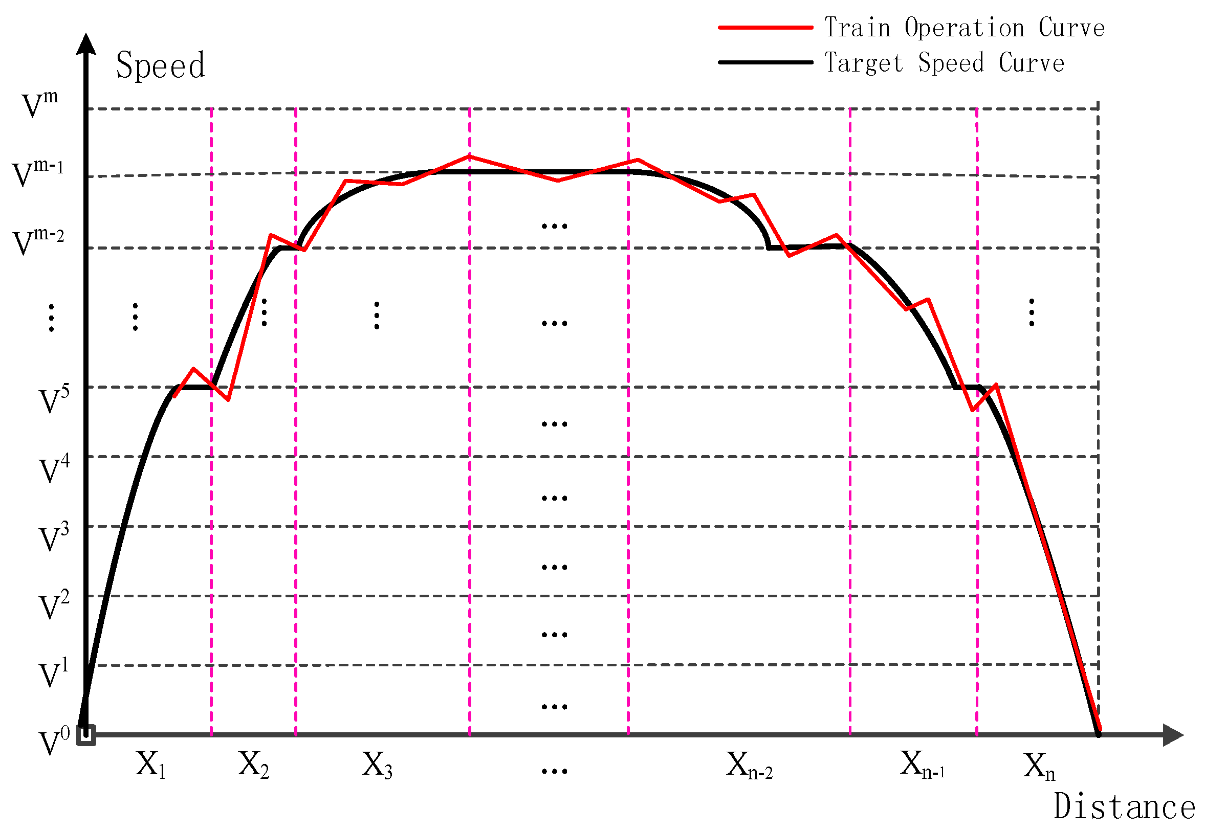
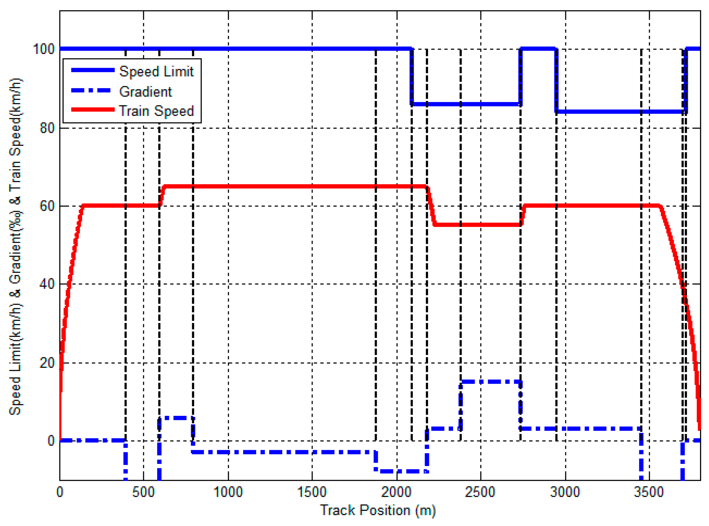
As shown in Figure 1, the object this paper researches is the train target speed curve, which needs to be calculated off-line in some literatures. The train reaches this target speed by traction, coasting or braking. Different operation mode is related to line conditions and running time constraints. The train tracks the target speed curve by cycles of traction-braking-coasting around the objective speed, but that problem is the optimization of ATO control, which is different with the problem this paper researches. The optimization of ATO control is also one of the hotspots in train energy-efficient operation research [30].

Therefore, the objective function of the energy-efficient train operation model is:

$$F_{ai}= M\times a_i+F_i^{br}+F_i^{gr}$$

(3)

$$F_{ci}= F_i^{br}+F_i^{gr}$$

(4)

$$E_i=F_{ai}\times S_i+F_{ci}\times D_i$$

(5)

$$E_{total}=min{\displaystyle \sum }_{i=1}^n{E}_i$$

(6)

where $M$ is the total mass of the train;$a_i$ is acceleration of the train in the $i$th interval;$F_i^{br}$ is the basic resistance of the train in the $i$th interval; $F_i^{gr}$ is the gradient resistance of the train in the $i$th interval; $F_{ai}$ is traction force in acceleration process of the train in the $i$th interval, $F_{ci}$ is traction force in cruising process of the train in the $i$th interval, $S_i$ is acceleration distance of the train of the $i$th interval; $D_i$ is cruising distance of the train in the $i$th interval; $E_i$ is tracking energy consumption in the $i$th interval; $E_{total}$ is the total energy that the train consumes after completing all discrete-points speed code selection (in kWh); and $n$ is the number of discrete points after discretization of the line.

Under normal circumstances, the running time of the train on the segments will strictly conform to the requirements of the schedule. The driving strategies will attempt to achieve the train operation and running times specified in the schedule are the same [31]. The driving strategy will also ensure that the actual operation time of the train is within the allowable difference between the two, even under extreme circumstances. Therefore, in the process of the algorithm design, the operation time needs to be constrained:

$$T_i=\frac{V_i-V_{i-1}}{a_i}+\frac{D_i}{V_i}$$

(7)

$$T={\displaystyle \sum }_{i=1}^n{T}_i$$

(8)

$$\left|T-T_{running}\right|\le \Delta t$$

(9)

where $T_i$ is the actual running time of the train in the $i$th interval; $a_i$ is acceleration of the train in the $i$th interval; $V_i$ is the tracking target speed code in the $i$th interval; $D_i$ is cruising distance of the train in the $i$th interval; $T$ is the actual total running time of the train (in seconds); $T_{running}$ is the running time according to the timetable scheduled requirements (in seconds); $\Delta t$ is the permissible value of the train running time, which is a positive value, $n$ is the number of discrete points after discretization of the line.

The ant ACO is modeled on ants’ foraging process in the natural world. Generally, the ants’ foraging space describes the problem search space and the ant colony can be regarded as a set of effective solutions to the search space, and ant paths are used to represent feasible solutions. Therefore each ant can independently search the problem space for feasible solutions. The pheromone will be left behind during the foraging process. Meanwhile, the pheromone in the path will evaporate as time goes by. Therefore, the ant will choose the right path through perceiving the pheromone concentration, and then by continuous iteration obtain the optimal solution. Finally, the ant colony will centralize to the optimal path, which is the optimal solution to the problem. The correspondence between actual ant phenomena and our model are shown in

Table 1. The corresponding elements table between ant colony foraging phenomenon and ant colony optimization algorithm.

Ant Colony Foraging Phenomenon	Ant Colony Optimization Algorithm
Ant colony	A set of effective solutions to the search space
Foraging space	Problem search space
Pheromone	Pheromone concentration
Path from nest to food	Effective solution
Found the shortest path	The optimal solution to the problem

.

By summarizing the above fundamental elements of the ACO algorithm, we can summarize its main features as follows:

• It possesses positive feedback, and heuristic hunting characters
• It uses distributed control but not centralized control
• It is has strong robustness
• Each individual can perceive only local information, but not global information

MAX-MIN Ant System (MMAS) is one of the most effective algorithms in ACO. In addition, focusing on the optimization of the energy-efficient train operation, compared with other optimization algorithms, MMAS has the following three advantages:

• It has good real-time performance of the energy-efficient train operation
• The setting of heuristic pheromone can effectively improve the convergence speed of the algorithm
• The method can avoid getting the local optical solution and has better search capabilities of global information

To the best of our knowledge, there is little research in energy-efficient train operation that uses the two-stage MMAS optimization algorithm. By considering the characteristics of the two-stage MMAS algorithm, and the present research conditions, using this algorithm is expected to expand on prevailing ideas and methods in the field of energy-efficient train operation.

3. Improved Ant Colony Algorithm Modeling

The ant colony optimization algorithm is motivated by simulating the process of ants foraging to solve discrete combination-optimization problems. The advantage of the ant colony optimization algorithm is that it is superior to other algorithms [32], as it is more effective in terms of computing speed and convenience. MMAS is a type of improved ACO algorithm that aims to solve a discrete optimization problem. It generally contains two important parts: path construction and pheromone updating. Therefore, the problem of energy-efficient train operation using MMAS is divided into two parts as respectively described in the following two sections.

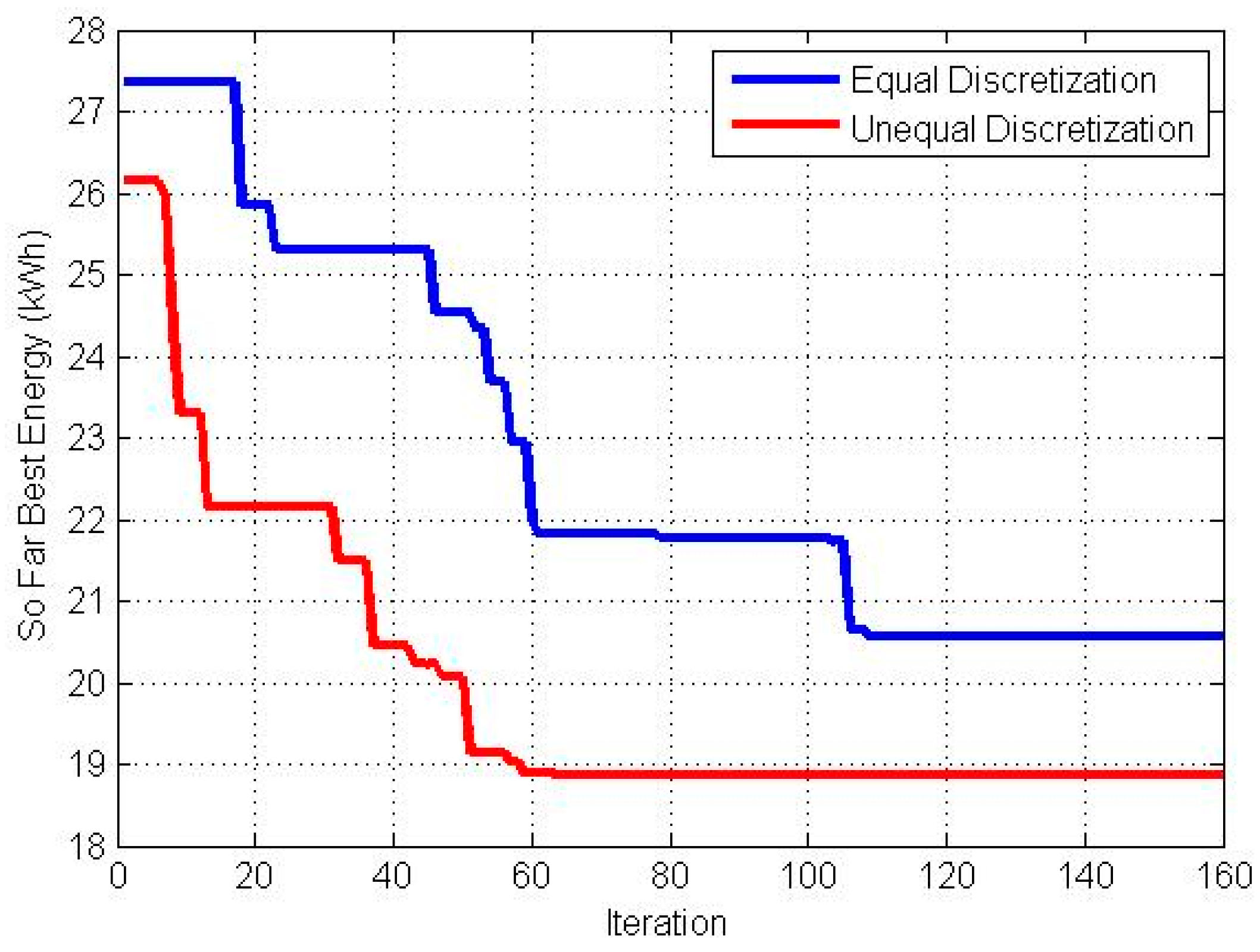
3.1. Partition of the Algorithm

Discretization in the ACO algorithm affects the size of the problem: a reasonable discretization can reduce the solution-space energy-saving train-operation optimization, and accelerate the convergence speed.

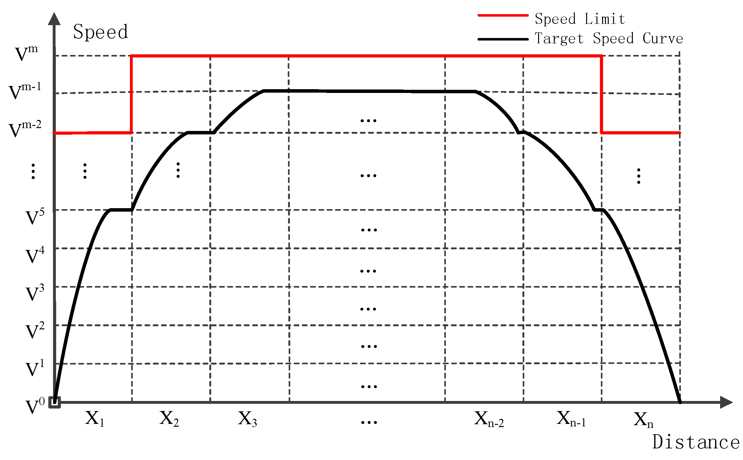
ACO algorithms usually use equal discretization when solving the discrete combination optimization problem. Figure 2 shows the equal discretization: the train can choose the corresponding target speed of every segment. A target speed sequence builds up a target speed curve.

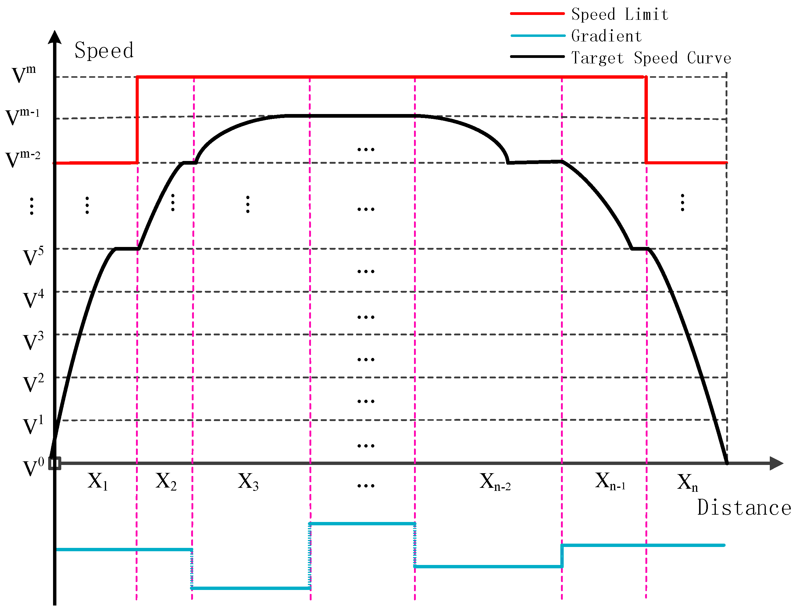
In reality, the line information and traffic operation characteristics must be taken into consideration. Therefore it discretizes the line into $n$ segments based on the variety of static gradient and speed limit. As shown in Figure 3, the speed limit and gradient in each discretized segment are constant, so that the algorithm can optimize conveniently.

3.2. Pheromone

The pheromone plays a guiding role for the algorithm allowing it to find the optimal speed profile. It reflects the effect of the a priori factors and the certainty factors and so is critical in the search process described herein. In this paper, the pheromone setting studies the driving experience of train drivers. The principle is as follows: taking the real driving experience into account, the train speed tends to accelerate when downhill and tends to decelerate when uphill. This principle affects the probability when searching the next path in solution space, can change the searching direction, accelerate the convergence rate of the algorithm, and improve the performance of the algorithm. Based on the two aspects of the improvement, a target speed curve optimization method based on MMAS is proposed in this paper.

3.3. Path Construction

Path construction uses random proportion rules to choose the next step: the random proportion rule of the MMAS algorithm is basically consistent with the earliest ant system (AS) algorithm, and the specific proportion random rule is defined as follows:

$$P_n\left(V_i,V_{i+1}\right)=\{\begin{array}{ll}\frac{\left(1-\gamma \right)\cdot \phi \left(V_i,V_{i+1}\right)+\gamma \cdot \rho \left(V_i,V_{i+1}\right)}{{{\displaystyle \sum }}_{ V_{j+1}\in I }[\left(1-\gamma \right)\cdot \phi \left(V_i,V_{j+1}\right)+\gamma \cdot \rho \left(V_i,V_{j+1}\right)}& V_{j+1}\in I\\ 0& other\end{array}$$

(10)

where $P_n\left(V_i,V_{i+1}\right)$ is the selection probability of the tracking target speed $V_{i+1}$ when the $n$th ant is in the $i$th discrete point to the $i+1$th discrete point; $\gamma$ is a constant value to regulate the proportion of pheromone trails and the heuristic information, with $0\le \gamma \le 1$; $\phi \left(V_i,V_{i+1}\right)$ is the heuristic information values for the tracking target speed $V_{i+1}$; $\rho \left(V_i,V_{i+1}\right)$ being the pheromone trail values of the tracking target speed $V_{i+1}$ when the $n$th ant is in the $i$th discrete point to the $i+1$th discrete point; $I$ is the collection of all the feasible tracking target speeds in the $i+1$th discrete point; n is the grade of the ant.

3.4. Pheromone Updating

In the MMAS algorithm, the pheromone updating rule has evolved significantly compared with traditional ACO. The MMAS algorithm focuses on the larger improvements of the pheromone updating, which enhances algorithm performance. The specific pheromone updating rule is defined as follows:

$$\rho \left(V_i,V_{i+1}\right)=\{\begin{array}{cc}\lambda \cdot \Delta {\rho }_n\left(V_i,V_{i+1}\right)+\left(1-\delta \right)\cdot {\rho }_n\left(V_i,V_{i+1}\right)& if ant is iteration-best\\ \left(1-\lambda \right)\cdot \Delta {\rho }_n\left(V_i,V_{i+1}\right)+\left(1-\delta \right)\cdot {\rho }_n\left(V_i,V_{i+1}\right)& if ant is so-far-best\\ \left(1-\delta \right)\cdot {\rho }_n\left(V_i,V_{i+1}\right)& other\end{array}$$

(11)

$$\Delta {\rho }_n\left(V_i,V_{i+1}\right)=\{\begin{array}{cc}{\left(\frac{E_{sbest}}{E_{ibest}}\right)}^{\tau } \hfill & \hfill if ant is iteration-best \\ 1\hfill & \hfill if ant is so-far-best\\ 0\hfill & \hfill other\end{array}$$

(12)

where $\rho \left(V_i,V_{i+1}\right)$ being the pheromone trail values of the tracking target speed $V_{i+1}$ when the $n$th ant is in the $i$th discrete point to the $i+1$th discrete point; $\Delta {\rho }_n\left(V_i,V_{i+1}\right)$ is the released pheromone trail values of the tracking target speed $V_{i+1}$ when the $n$th ant is in the $i$th discrete point to the $i+1$th discrete point; $\lambda$ is the weighting factor of the iteration-best solutions, with $0<\lambda <1$; $1-\lambda$ is the weighting factors of the best-so-far solutions; $\delta$ is the pheromone evaporation rate, with $0<\delta \le 1$; $\tau$ is a constant which can be set to determine whether a pheromone is initialized again; $E_{ibest}$ is the minimum energy consumption in this iteration (in kWh); $E_{sbest}$ is the minimum energy consumption so far (in kWh). The process of line discretization is described as follows:

Step 1.

Import line data containing the gradients and speed limits, and initialize the related parameters;

Step 2.

Set the discretization density, and then discretize lines and running target speeds;

Step 3.

Calculate the equivalent value based on the gradient data;

Step 4.

Calculate the energy-consumption and running time, including the train starting phase, train running phase and train braking phase;

Step 5.

Store the data and create the energy consumption and running time lookup table;

Step 6.

Output the lookup table.

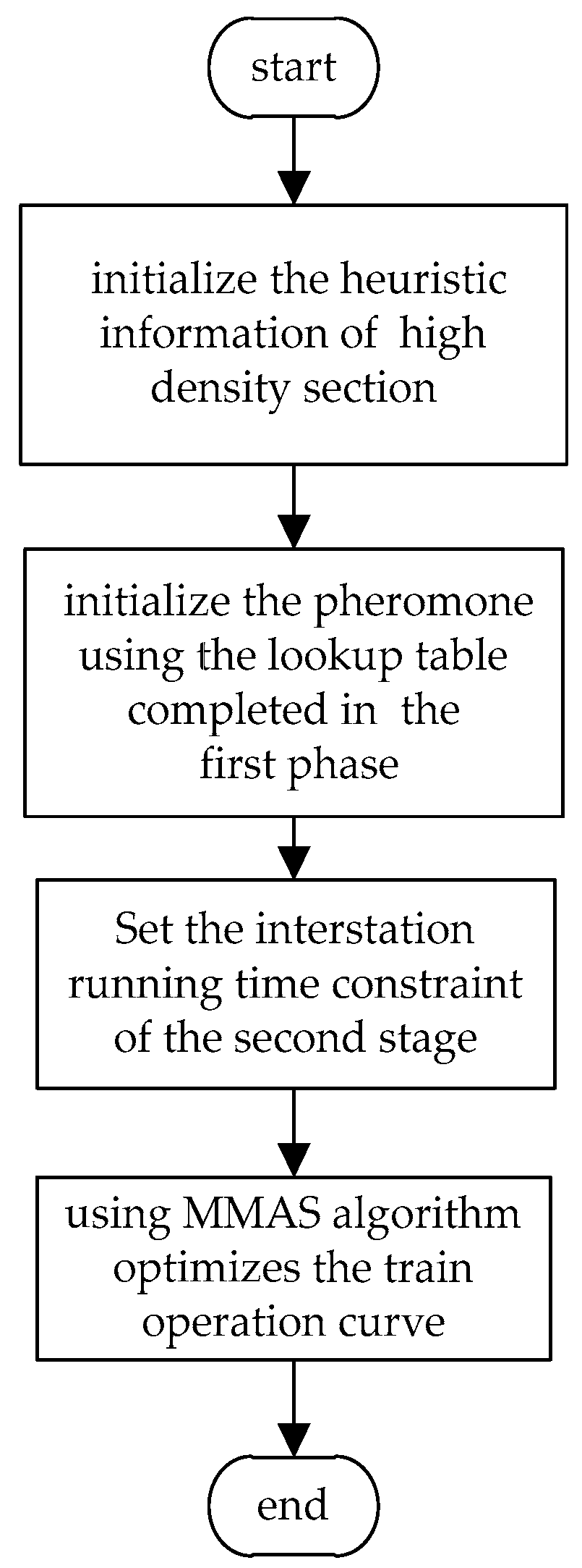
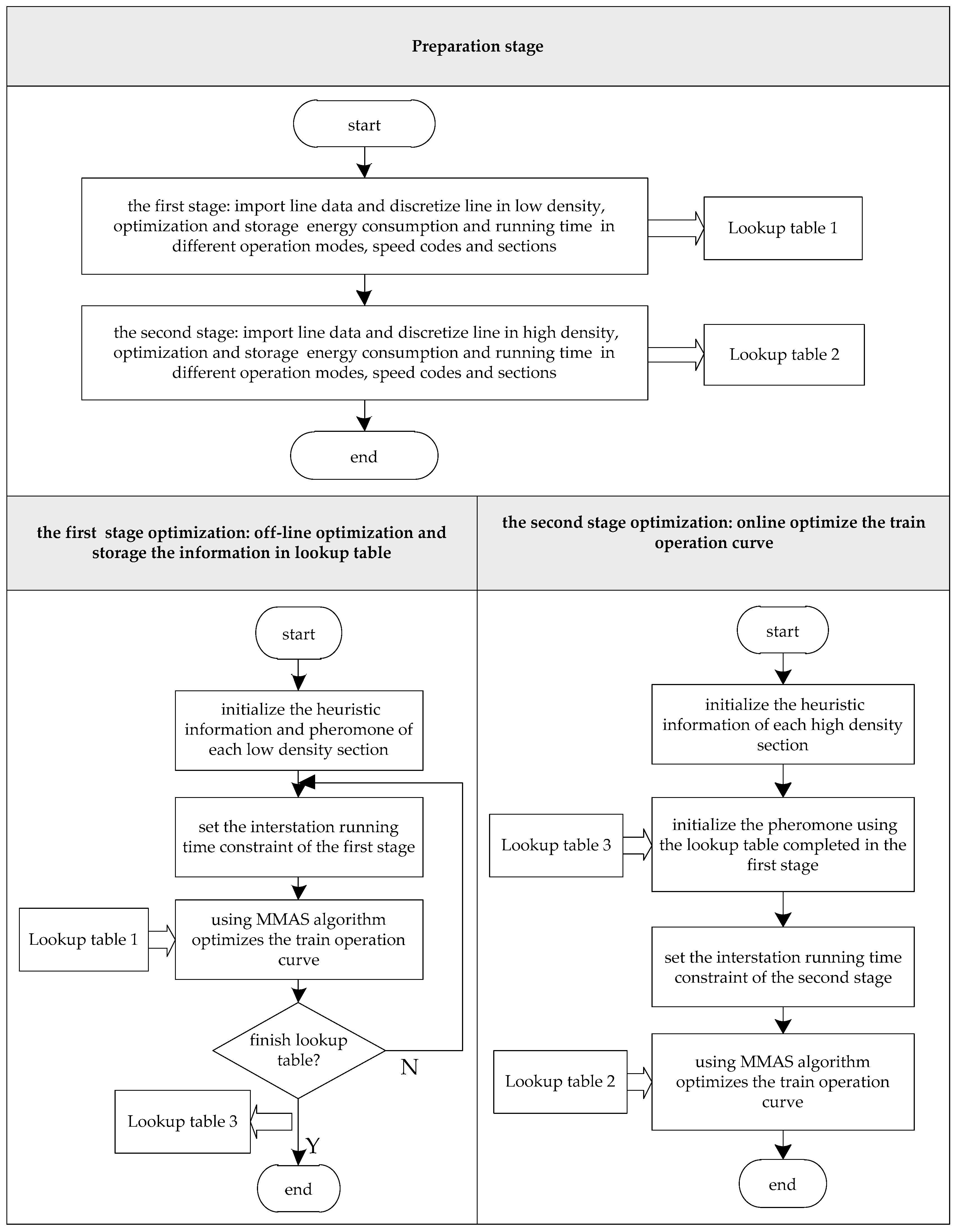
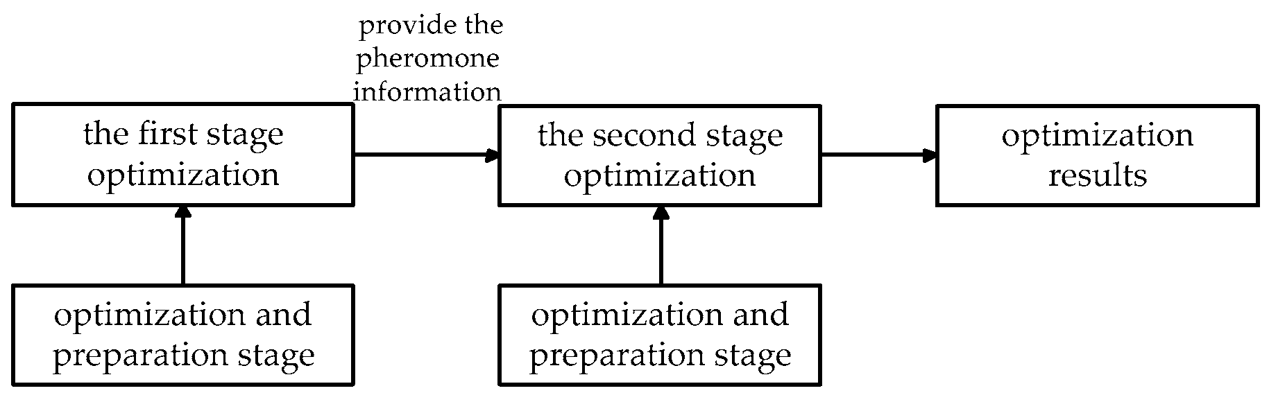
The above provides a concrete model for the discrete optimization and the MMAS algorithm, which lays the foundations for the design of train energy-saving speed curve optimization based on a two-stage optimization algorithm. The first stage, i.e., low density discretization, is fully optimized to search for the best solution; the second-stage, i.e., high density discretization, will refer to the first stage information and quickly search for the optimal solution. The algorithm design is described in the following section.

4. Overall Design of Improved ACO

In terms of energy-efficient train operation [13], the train needs to accelerate at the beginning and brake on arrival. When the train is running between stations, the train uses a combination of accelerating, cruising, coasting and braking. To achieve this, the algorithm is designed to use the optimization results from the first phase as a reference for second stage optimization. This means that two stages of optimization design are needed and both use the MMAS algorithm. In the first stage, we divide the subway line to achieve low-density discretization; in the second stage, we derive a high density discretization to search for the more viable path. The second stage of high-density discretization therefore cuts the line into many small lengths with the aim of searching the optimal path as accurately and fast as possible. The results of the first stage will already have converged to the vicinity of the optimal path and the high-density discrete optimization simulation of the second stage takes full advantage of that to initialize the optimization of pheromone values. The second stage therefore finds a better path in the shortest time, improving the efficiency of the overall optimization and improving real-time performance. The overall architecture is further illustrated by Figure 4.

4.1. Preparation of Optimized Stage

The main purposes in preparing the optimization stage are to discretize running lines and target speed for the train, form different operating modes and the corresponding energy consumptions under different target speeds, and establish a look-up table of running times. The look-up table allows the optimization stage to search different operation modes and target speeds in each discrete section, in order to prepare for efficient optimization.

4.2. Optimization of the First Stage

The main functions of the optimized first stage are to search every possible running path of the train constructed in the prepared optimization phase, being as comprehensive as possible, find the qualifying paths, then gradually converge to the optimal path and finally save all the pheromone information for the path. In addition, the look-up table of pheromones for optimization of the second stage is also built.

Then the ACO needs to set heuristic pheromone in the initialization phase. The strategies for heuristic pheromone in this design are set by referring to the experience of train drivers. The main setting principles are described as: take the real driving experience into account, the train speed tends to accelerate when downhill and tends to decelerate when uphill. The detailed process of the first-stage optimization is shown in Figure 5.

4.3. Optimization of the Second Stage

The center operators would change in real-time the planned interstation running time according to when the train arrived at the station early or late, so we need to further optimize the target speed curve in the second stage. Second-stage optimization mainly considers two factors:

• Whether the route searching is comprehensive
• Whether the optimization time is fast enough

We mainly consider the first factor during the first stage and provide reference information for optimization of the second stage. The second factor will be mainly considered during the second stage. The result of the low-density first-stage optimization will have already provided an approximation of what is optimal. The pheromone look-up table formed after the end of optimization is used as the value for the pheromone initialization. This improves the pheromone distribution when searching paths during optimization of the second stage. Note that the optimization of the second stage involves high-density discretization and we have a better search direction at the beginning of optimization. Therefore, according to this design, the optimized speed of the second stage will be further improved, and the optimized time will be significantly reduced. The procedure of the second stage is shown in Figure 6. The set strategy for heuristic pheromone in this optimization stage is achieved in the same way as the first stage, and we also add the train drivers’ driving experience.

4.4. Overall Design

The overall design process of the train energy-saving optimization simulation is shown in Figure 7.

5. Simulations Based on Beijing Subway Changping Line

5.1. Basic Data

To illustrate the effectiveness of the proposed model and algorithm, a case based on the Beijing subway Changping line is provided as an example. The chosen line covers a length of 3800 m, consisting of two stations and one interstation. The practical running time is 246 s and the energy consumption for this interstation trip is 21.62 kWh. As shown in

Table 2. The slope data of the simulation cases.

Starting Position (m)	Final Position (m)	Slope (Micrometer Degrees)
0	398	0
398	598	−23.835
598	798	5.6
798	1878	−3
1878	2184	−7.99
2184	2386	2.971
2386	2739	14.873
2739	3453	3
3453	3698	−12.449
3698	3800	0

and

Table 3. The speed limit data of the simulation cases.

Starting Position (m)	Final Position (m)	Speed Limit Value (km/h)
0	2092	100
2092	2739	86
2739	2949	100
2949	3719	84
3719	3800	100

respectively, the subway line data derived from Beijing subway Changping line contains static gradients, and speed limits. The train speed code is partitioned from 40 km/h to 100 km/h every 5 km/h, as shown in

Table 4. The partition of speed code data.

Speed Code	V1	V2	V3	V4	V5	V6	V7	V8	V9	V10	V11	V12	V13
Speed value	40	45	50	55	60	65	70	75	80	85	90	95	100

. In the case study, the train formation form is three motor cars (M1, M2 and M3) and three trailer cars (T1, T2 and T3), the total mass of the train is 199 t, as shown in

Table 5. Weight of the vehicles.

Vehicle	T1 (t)	M1 (t)	T2 (t)	M2 (t)	M3 (t)	T3 (t)	Total (t)
Weight	33	35	28	35	35	33	199

.

Table 6. Parameters of MMAS.

Parameters Names	Parameters Values
Iteration	160
The number of ants	30
The maximum of pheromone	9.99
The minimum of pheromone	0.01
The pheromone evaporation rate	0.05
The weighting factor of the iteration-best solutions	2.3
The weighting factors of the best-so-far solutions	2.1
The proportion of pheromone trails and the heuristic information	0.7

shows the parameters of MMAS.

5.2. The First Stage Simulation Result

By using the method proposed above, the speed profile is optimized based on the constraints of the running time.

Figure 8 shows the first stage convergence analysis from the algorithm. In the problem solution space, with the increasing of iterations, the so far best energy and the iteration average energy decrease gradually and remain stable at about the 60th and 110th generation, respectively. After the first stage optimization, a nearly globally optimal solution has been obtained.

Figure 9 illustrates that the algorithm obtains the first stage optimal speed profile. According to the gradient and the speed limit data, the interval has been discretized into 13 sections. Each section has a constant gradient and speed limit value. The train gains traction when starting and brakes when approaching a station. In the other sections, the train uses different operation modes.

5.3. The Second Stage Simulation Result

In this case, according to the practical train operation in the Changping Line, the planning running time has been adjusted to 251 s. Figure 10 shows the second stage optimization iteration convergence. Based on the first stage optimization results, MMAS searches for the optimal solution near the first stage optimal solution. The so far the best energy and the iteration average energy decrease gradually and remain stable at about the 5th and 60th generation, respectively, which reflects fast convergence.

Figure 11 describes the second stage optimal speed profile. Based on the first stage discretization, the second stage discretizes the line into 21 sections. Compared with the first stage optimal speed profile, the second stage optimal speed profile has some differences in operation modes, but the general tendency is approximately the same.

The simulation results don’t have too many coasting sections as described in the literature, because the data is derived from practical operation based on the Beijing subway Changping line, and not only to meet the requirements of running time interstation, but also to meet the requirements of the higher technical speed.

Table 7. Comparison between the result of the first stage and the second stage.

Optimization Stage	Planning Running Time (s)	Running Time (s)	Energy Consumption (kWh)	Computing Time (s)
The first stage	246	242.71	18.87	39.67
The second stage	251	248.05	18.61	19.58

shows the comparison between the result of the first stage and the second stage. The running times are 242.71 s and 248.05 s, respectively, which both satisfy the operation requirements of the timetable. The second stage is online optimization, and the algorithm optimization time is 19.58 s, while the dwell time is 30 s. The optimization time is smaller than the dwell time, so the energy-efficient speed profile for the next interstation can be quickly obtained during the dwell time. It indicates that the algorithm has the capability of fast optimization of the speed profile.

In

Table 8. Comparison between simulation results and practical data.

Results	Planning Running Time (s)	Running Time (s)	Energy Consumption (kWh)	Computing Time (s)
Practical data	246	245.00	21.62	–
Simulation result	251	248.05	18.61	19.58

, the simulation results and practical data are compared to verify the effectiveness of the optimization method used herein. The results illustrate that the algorithm can quickly obtain the energy-efficient speed profile under the constraint of running time. Significant energy saving effects are achieved: the energy saving rate is 13.92%.

6. Influence of Different Factors on Simulation

6.1. Improvement Based on Partition

The discretization of MMAS influences the convergence rate and the energy-efficient rate very much. This paper discretized the line based on gradients and speed limits. To verify the effect of our algorithm a comparison between equal discretization algorithms (as shown in Figure 12) and unequal discretization algorithms (as shown in Figure 9) is made. The difference between the two algorithms is simply the discretization method, other parameters remaining the same in order to ensure the effectiveness of the comparison.

As shown in Figure 13, the equal discretization and unequal discretization so far best energy decrease gradually and keep stable at about 110th and 60th generation respectively. Unequal discretization can achieves better convergence and energy-efficient performance.

As shown in

Table 9. Comparison between equal discretization and unequal discretization.

Discretization Method	Planning Running Time (s)	Running Time (s)	Energy Consumption (kWh)	Computing Time (s)
Equal discretization	246	243.25	20.57	81.20
Unequal discretization	246	242.71	18.87	39.67

, while the practical running time is 246 s, the optimal running times of the two algorithms are 243.25 s and 242.71 s, which both satisfy the operation requirements of the timetable. The energy consumption of the unequal discretization algorithm is 18.87 kWh, which is smaller than the energy consumption of the equal discretization algorithm. Also, the computation time of the unequal discretization algorithm is much smaller than that of the equal discretization algorithm. This indicates that the unequal discretization algorithm achieves better real-time performance. Therefore, unequal discretization of the line is shown to be needed.

6.2. Improvement Based on Driving Experience

In this study heuristic pheromone values were set as shown in

Table 10. Heuristic pheromone setting based on driving experience.

Gradient Value	Heuristic Pheromone Weighting Value
	Accelerate	Cruise	Decelerate
>0	$0.2$	$0.5$	$0.8$
=0	$0.3$	$0.7$	$0.3$
<0	$0.8$	$0.5$	$0.2$

, which were derived through study of driver experience: the train speed tends to accelerate when downhill and tends to decelerate when uphill.

The heuristic pheromone influences the probability of searching-ants search finding a path in the solution space and changes the search direction of the ants. In order to verify the effects of these heuristic pheromone settings, a comparison between two heuristic pheromone settings has been made, other heuristic parameters remaining the unchanged in order to ensure the effectiveness of the comparison.

The algorithm in this paper obtained the optimal speed profile with constant value heuristic pheromone setting (Figure 14) and driver experience (Figure 9). As shown in Figure 15, the constant value heuristic pheromone setting and with driving experience heuristic pheromone setting have different so far best energy convergence, decrease gradually and remain stable at about 80th and 60th generation respectively.

Table 11. Comparison between different heuristic pheromone settings.

Heuristic Pheromone	Energy Consumption (kWh)	Computing Time (s)
Constant value	19.54	67.53
Driving experience	18.87	39.67

shows the energy consumption and computing time comparison between different heuristic pheromone settings. The pheromone settings based on driving experience achieve better real-time and energy-efficient performance. Therefore, our improved method is shown to have significant potential for improving the computation rate and so aid in incorporating optimized target speed curves into real-time rail systems.

7. Conclusions

In CBTC systems, the center operators would change in real-time the planned running time of interstation segments according to whether the train arrived at the station early or late, so it is a very important problem to consider the real-time properties in the process of train energy-efficient operation. Aiming at the problem that is abstracted from a practical subway line, this paper proposes a discrete-combined model based on linear approximation calculations to optimize train energy-efficient operation. According to the static gradient and the speed limit, the line is unequally discretized in low density in the first stage and in high density in the second stage, and each stage has different running time restrictions. Based on the operation data from the Beijing subway Changping line, the simulation results shows that the energy consumption is reduced by 13.92% after two stage MMAS optimization. The second stage optimization time is 19.58 s, which shows good energy-efficient and real-time performance compared with the method used in previous researches. With the decrease of train headway in the CBTC system, research on the process of multi-train energy saving operation also needs to be considered in the real-time running time changes of each train, and this will be a topic in our future research.

References

1. Ishikawa, K. Application of optimization theory for bounded state variable problems to the operation of trains. Bull. JSME Nagoya Univ. 1968, 11, 857–865. [Google Scholar] [CrossRef]
2. Howlett, P. Optimal strategies for the control of a train. Automatica 1996, 32, 519–532. [Google Scholar] [CrossRef]
3. Cheng, J.X.; Howlett, P. A note on the calculation of optimal strategies for the minimization of fuel consumption in the control of trains. IEEE Trans. Autom. Control 1993, 38, 1730–1734. [Google Scholar] [CrossRef]
4. Howlett, P.G.; Pudney, P.J. Energy-Efficient Train Control; Springer: London, UK, 2012. [Google Scholar]
5. Wang, F.; Liu, H.D.; Ding, Y.; Chen, S.L.; Mao, B.H. Arithmetic and Application Technology of Train Energy-Economizing Movement. J. North. Jiaotong Univ. 2002, 26, 13–18. [Google Scholar]
6. González-Gil, A.; Palacin, R.; Batty, P.; Powell, J.P. A systems approach to reduce urban rail energy consumption. Energy Convers. Manag. 2014, 80, 509–524. [Google Scholar] [CrossRef]
7. Ding, Y.; Mao, B.H.; Liu, H.D.; Wang, T.C.; Zhang, X. An Algorithm for Energy-Efficient Train Operation Simulation with Fixed Running Time. J. Syst. Simul. 2004, 16, 2241–2244. [Google Scholar]
8. Ding, Y.; Mao, B.H.; Liu, H.D.; Zhang, X.; Wang, T.C. Study on Train Movement Simulation for Saving Energy. J. North. Jiaotong Univ. 2004, 28, 76–81. [Google Scholar]
9. Liu, H.D.; Mao, B.H.; Ding, Y.; Jia, W.Z.; Lai, S.K. Train Energy-saving Scheme with Evaluation in Urban Mass Transit Systems. J. Transp. Syst. Eng. Inf. Technol. 2007, 7, 68–73. [Google Scholar] [CrossRef]
10. Fu, Y.P.; Li, K.P. Optimal Method of Train Saving Energy Operation. Sci. Technol. Eng. 2009, 9, 1337–1340. [Google Scholar]
11. Howlett, P.G.; Pudney, P.J.; Vu, X. Local energy minimization in optimal train control. Automatic 2009, 45, 2692–2698. [Google Scholar] [CrossRef]
12. Ke, B.R.; Lin, C.L.; Lai, C.W. Optimization of Train-Speed Trajectory and Control for Mass Rapid Transit Systems. Control Eng. Pract. 2011, 19, 675–687. [Google Scholar] [CrossRef]
13. Dong, Y.; Liu, H.; Bai, Y.; Zhou, F.M. A Two-level Optimization Model and Algorithm for Energy-Efficient Urban Train Operation. J. Trans. Syst. Eng. Inf. Technol. 2011, 11, 96–101. [Google Scholar] [CrossRef]
14. Domínguez, M.; Fernández-Cardador, A.; Cucala, A.P.; Gonsalves, T.; Fernandez, A. Multi objective particle swarm optimization algorithm for the design of efficient ATO speed profiles in metro lines. Eng. Appl. Artif. Intell. 2014, 29, 43–53. [Google Scholar] [CrossRef]
15. Huang, Y.; Ma, X.; Su, S.; Tang, T. Optimization of Train Operation in Multiple Interstations with Multi-Population Genetic Algorithm. Energies 2015, 8, 14311–14329. [Google Scholar] [CrossRef]
16. Zhao, N.; Roberts, C.; Hillmansen, S.; Nicholson, G. A multiple train trajectory optimization to minimize energy consumption and delay. IEEE Trans. Intell. Transp. Syst. 2015, 16, 2363–2372. [Google Scholar] [CrossRef]
17. Li, Z.Y.; Wei, X.K.; Wang, H.; Jia, L.M. Optimizing power for train operation based on ACO. In Proceedings of the International Conference on Electrical and Information Technologies for Rail Transportation, Zhuzhou, China, 28–30 August 2015; pp. 453–462.
18. Ke, B.R.; Chen, M.C.; Lin, C.L. Block-Layout Design Using MAX-MIN Ant System for Saving Energy on Mass Rapid Transit Systems. IEEE Trans. Intell. Transp. Syst. 2009, 10, 226–235. [Google Scholar]
19. Ke, B.R.; Lin, C.L.; Yang, C.C. Optimization of Train Energy-Efficient Operation for Mass Rapid Transit Systems. IET Intell. Transp. Syst. 2011, 6, 58–66. [Google Scholar] [CrossRef]
20. Wong, K.K.; Ho, T.K. Dynamic coast control of train movement with genetic algorithm. Int. J. Syst. Sci. 2004, 35, 835–846. [Google Scholar] [CrossRef] [Green Version]
21. Miyatake, M.; Ko, H. Optimization of Train Speed Profile for Minimum Energy Consumption. IEEE Trans. Electr. Electron. Eng. 2010, 5, 263–269. [Google Scholar] [CrossRef]
22. Jin, W.D.; Jin, F.; Li, C.W.; Hu, F.; Gou, X.T. Study on Intelligent Computation of Velocity Schema Curve of Optimization Operation for Train. J. China Railw. Soc. 1998, 20, 47–52. [Google Scholar]
23. Su, S.; Li, X.; Tang, T.; Gao, Z.Y. A subway train timetable optimization approach based on energy-efficient operation strategy. IEEE Trans. Intell. Transp. Syst. 2013, 14, 883–893. [Google Scholar] [CrossRef]
24. Su, S.; Tang, T.; Li, X.; Gao, Z.Y. Optimization of multitrain operations in a subway system. IEEE Tran. Intell. Transp. Syst. 2014, 15, 673–684. [Google Scholar]
25. Sicre, C.; Cucala, A.P.; Fernández-Cardador, A. Real time regulation of efficient driving of high speed trains based on a genetic algorithm and a fuzzy model of manual driving. Eng. Appl. Artif. Intell. 2014, 29, 79–92. [Google Scholar] [CrossRef]
26. Yin, J.; Chen, D.; Li, L. Intelligent train operation algorithms for subway by expert system and reinforcement learning. IEEE Trans. Intell. Transp. Syst. 2014, 15, 2561–2571. [Google Scholar] [CrossRef]
27. Khmelnitsky, E. On an optimal control problem of train operation. IEEE Trans. Autom. Control 2000, 45, 1257–1266. [Google Scholar] [CrossRef]
28. Gu, Q.; Tang, T.; Ma, F. Energy-Efficient Train Tracking Operation Based on Multiple Optimization Models. IEEE Tran. Intell. Transp. Syst. 2016, 17, 882–892. [Google Scholar] [CrossRef]
29. Yang, X.; Li, X.; Ning, B.; Tang, T. A survey on energy-efficient train operation for urban rail transit. IEEE Trans. Intell. Transp. Syst. 2015, 17, 2–13. [Google Scholar] [CrossRef]
30. Su, S.; Tang, T.; Chen, L.; Liu, B. Energy-efficient train control in urban rail transit systems. Proc. Inst. Mech. Eng. Part F J. Rail Rapid Transit 2015, 229, 446–454. [Google Scholar] [CrossRef]
31. Liu, R.R.; Golovitcher, I.M. Energy-efficient operation of rail vehicles. Transp. Res. Part A Policy Pract. 2003, 37, 917–932. [Google Scholar] [CrossRef]
32. Dorigo, M.; Birattari, M.; Stützle, T. Ant colony optimization. IEEE Comput. Intell. Mag. 2006, 1, 28–39. [Google Scholar] [CrossRef]
Figure 1. Target speed curve and train operation curve.
Energies 09 00626 g001
Figure 2. Equal discretization.
Energies 09 00626 g002
Figure 3. Unequal discretization.
Energies 09 00626 g003
Figure 4. Overall architecture diagram of the train energy-efficient operation optimization simulation.
Energies 09 00626 g004
Figure 5. First stage optimization flow chart.
Energies 09 00626 g005
Figure 6. Second stage optimization flow chart.
Energies 09 00626 g006
Figure 7. The overall design process.
Energies 09 00626 g007
Figure 8. The first stage optimization iteration convergence.
Energies 09 00626 g008
Figure 9. The V-S curve of the first stage optimization.
Energies 09 00626 g009
Figure 10. The second stage optimization iteration convergence.
Energies 09 00626 g010
Figure 11. The V-S curve of the second stage optimization.
Energies 09 00626 g011
Figure 12. The V-S curve based on equal discretization algorithms.
Energies 09 00626 g012
Figure 13. Equal discretization convergence and unequal discretization convergence.
Energies 09 00626 g013
Figure 14. The V-S curve based on constant value pheromone setting.
Energies 09 00626 g014
Figure 15. Constant value convergence and driving experience convergence.
Energies 09 00626 g015