2. Related Work
A linear programming based technique for residential energy management is proposed in [
10]. This approach efficiently reduces the electricity cost and PAR. Moreover, user comfort is also increased by reducing appliance waiting time, however, price flexibility is not taken into account. In [
11], linear programming technique is used to solve residential energy management problem. This approach is efficient in terms of electricity cost reduction, however, more computational power is required to solve complex optimization problem. Moreover, linear programming based optimization technique only solve the load having linear characteristics. In [
12], authors use a monotonic optimization techniques to solve appliance scheduling problem. In this technique, renewable energy is used along with grid energy to fulfill energy demand during critical peak hours. Although, renewable energy is beneficial in reducing PAR and electricity cost however, this increases the integration complexity in the system. Considering variable loads, a mixed integer linear programming approach is used for cost efficient scheduling [
13]. In general, these techniques are efficient in reducing electricity cost of the end users along with PAR reduction. However, these techniques are computationally expensive and user comfort is not modeled.
On the other hand, heuristic optimization techniques are widely used to solve energy optimization problems in SG. These techniques are efficient in solving both linear and nonlinear energy optimization problems. In [
14], an optimal stoping rule based technique is used to schedule appliances. The authors model user comfort in terms of appliance waiting time cost. This technique works on different thresholds defined by users, and these thresholds are measured when electricity price signal is uniformly distributed. The scheme is efficient in real time price (RTP) environment and for limited number of appliances. In [
15], the authors categorized appliances on the bases of user comfort and electricity cost reduction. Mathematical models for each class of appliances are proposed where electricity cost reduction and user comfort are considered as a joint problem which is solved by using wind driven optimization (WDO) algorithm. For PAR and electricity cost reduction, Knapsack-wind driven optimization (K-WDO) is also proposed. Although, the proposed techniques are efficient in handling user comfort and electricity cost reduction. However, (
tc) appliances such as air-conditioner, and other user dependant appliances are not considered because inconsideration of thermal and occupancy constraints makes the working of these appliances are difficult to optimize.
Due to the unpredictable nature of distributed renewable energy sources and loads results non-linear problem in a large scale. To manage the operational cost of power plant, particle swan optimization (PSO) algorithm has been used in [
16]. In [
17], a heuristic based evolutionary algorithm (EA) has been used to schedule a large number of home appliances to reduce electricity cost and high peaks. Three service areas including residential, commercial and industrial are considered to perform simulations. Based upon real time pricing, appliance scheduling for cost reduction objective is performed using stochastic and robust optimization techniques [
18]. On the bases of energy demand and temporal characteristics, the appliances are categorized into deferrable, non-deferrable, interruptible and non-interruptible ones. These techniques [
16,
17,
18] are efficient in reducing electricity cost. However, user comfort is neglected which is major objective of the proposed work. In [
7,
19], both linear programming and game theoretic techniques for centralized and distributed energy management are proposed. PAR reduction and its effects on generation efficiency are also analyzed.
In [
20], authors propose a load control technique for multiple residential units where utility company use a cost function to provide electricity to end users. Users have been assigned different types of loads alongwith consumption limits and bounds. For this purpose, utility and end users communicate via AMI in order to schedule generation and consumption. In [
21], game theoretic approach is used to optimize energy consumption patterns of appliances. Authors stated that there is a tradeoff between user comfort and electricity cost reduction. User comfort and cost reduction objectives are handled in a simple way such that users are given priority to choose either comfort or cost reduction.
In [
22], energy management by controlling the thermostat of appliances is discussed. The thermostat of the appliance is controlled as per customer preferences to maintain the temperature in a desired limit. These types of approaches are efficient in terms of both cost and energy, however, it is difficult to tackle all the thermal constraints and parameters when different types of appliances are used. In [
23], HVAC scheduling scheme is proposed. To maximize the user comfort, thermal constraints are considered in the optimization problem. For this purpose, thermodynamic model of a house is proposed to control the temperature. Moreover, this scheduling problem is solved by using nonlinear optimization techniques. In [
24,
25], user comfort is taken into consideration by controlling thermostats according to desired temperature set points. By making thermostats more intelligent, appliances can be controlled more efficiently, because appliances only operate when needed. Similarly, Blerim et al. [
26] added intelligence to conventional programmable communication thermostats (CPCTs) by scheduling appliances via machine learning and wireless sensors. Along with electricity cost, energy consumption is also reduced as compared to other scheduling schemes where the primary objective was to reduce electricity cost only. Furthermore, user comfort is also maximized because once the pattern is learnt, energy management controller (EMC) takes actions according to energy demand and user preferences. In conclusion, some of the existing techniques are useful in reducing electricity cost while others are comfort aware. However, none of the techniques is efficient in scheduling appliances based on customers presence, weather conditions, and price signals. Therefore, to efficiently manage the energy consumption through appliance scheduling, all possible constraints must be taken into consideration.
In this paper, our main objective is to reduce the electricity cost of end users by scheduling home appliances while maintaining user comfort and PAR. Based on type, the household appliances are either controlled by intelligent thermostat or a controller which is run by GA. Various types of household appliances are considered where some are controlled by intelligent thermostats while other ones are controlled by using GA. For user comfort, appliance waiting is considered and iel appliances are used having fixed time delay set by users. Furthermore, user can set waiting time to minimum time slots according to his desire. On the other hand, knapsack capacity limit is imposed in optimization problem to reduce PAR. In each time slot, optimization algorithm schedules the appliances under capacity limit. Simulation results show that proposed algorithms achieve maximum electricity cost saving and average user comfort while minimizing the PAR.
3. System Model
We consider a residential unit where users share common energy source provided by utility. Each user has different types of
n appliances with variable energy consumption requirements. On the bases of user requirements, these appliances are categorized into
tc,
ua,
el,
iel, and
r. Within these categories, some appliances are shiftable having the objective of cost reduction. While, some appliances have strict schedules with aim at maximizing end user comfort.
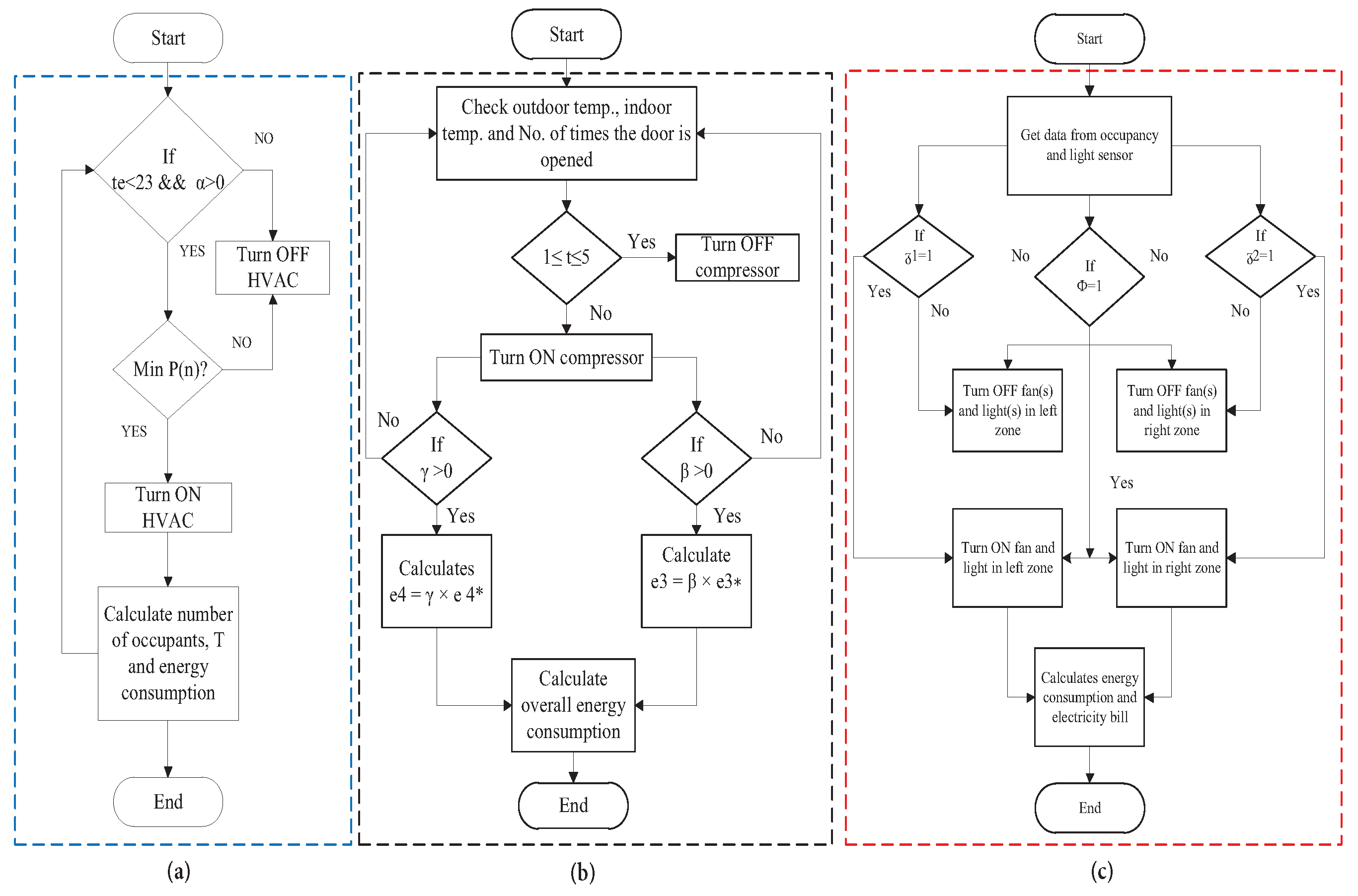
Figure 1 shows a schematic diagram of
tc and
ua appliances which are controlled by considering user occupancy and thermal constraints. The EMC uses the mathematical models of these appliances (
Section 3.3), user preferences and external parameters (i.e., price signal, user presence and temperature set points) to generate the optimization schedules for a given time interval
. On the other hand,
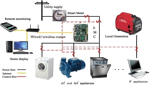
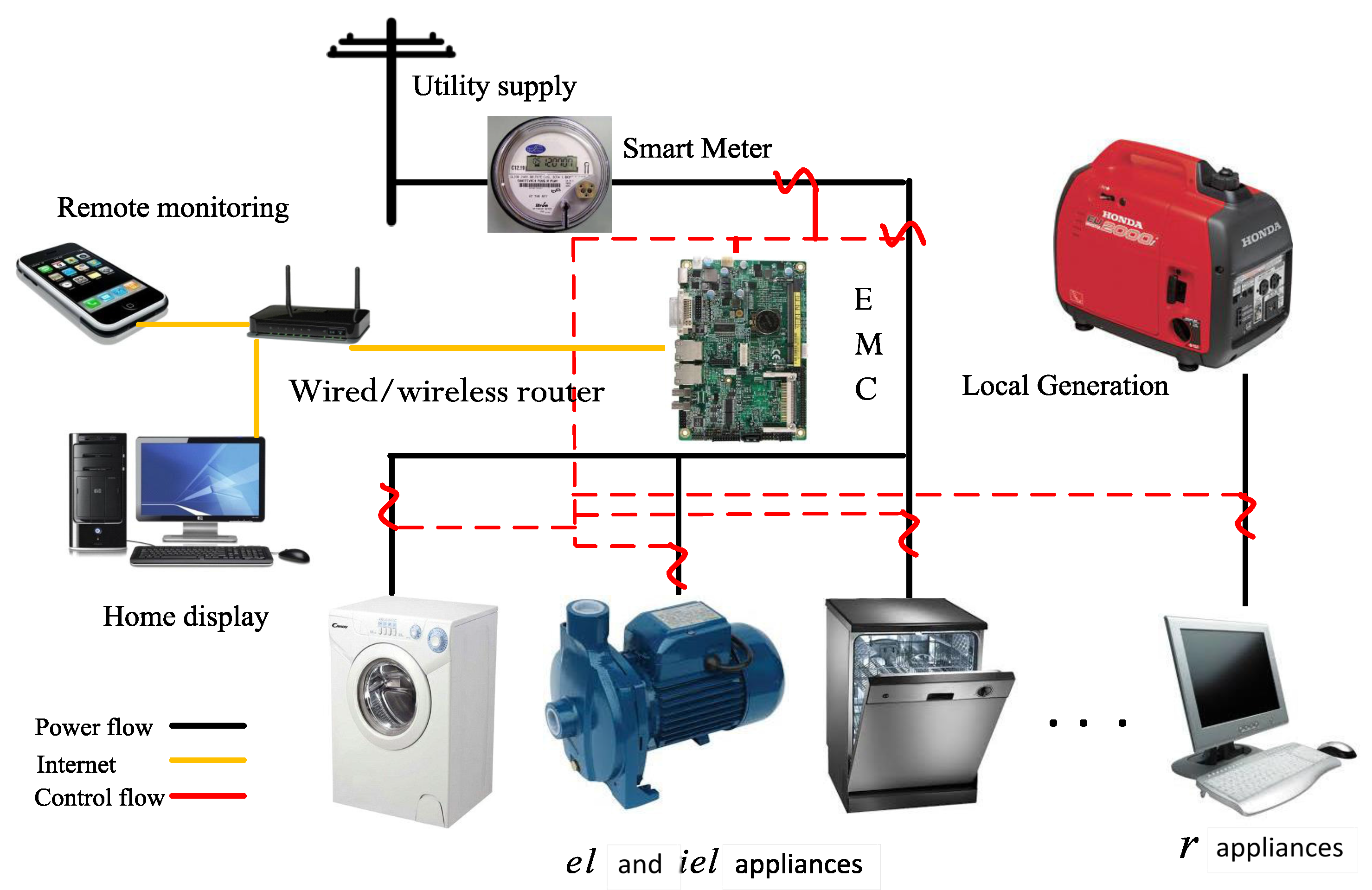
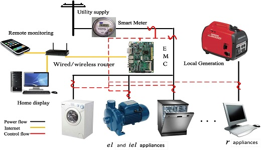
Figure 2 shows an architecture of
el,
iel, and
r appliances. Here, the energy demand of
r appliances is fulfilled through electricity generated from local generator (microgrid,
Section 3.1). This is because these are continuously running appliances which are difficult to schedule through optimization algorithms, hence do not take part in demand response (DR) programs. On the other hand,
el and
iel are scheduleable appliances and energy demand of these appliances is fulfilled through energy provided by utility company [
25]. Moreover, the scheduling horizon and operating hours of all the appliances can vary and usually depend on the user preferences and appliance type. So, prior to the formulation of electricity cost reduction objective function, classification of appliances, user comfort and energy generation are discussed along with their constraints. More importantly, the proposed model is generic in nature and appliances considered in these categorization are not fixed. Any one who want to use this model can add or remove any appliances according to his own requirements.
3.1. Energy Generation Model
A microgrid contains localized electricity sources i.e., diesel generators and renewable energy and loads. Loads normally connected with traditional grid (macrogrid). However, with the economic and physical conditions, it can be disconnected from macrogrid [
27]. In the proposed work, we use localized diesel power generator operated at minimum fuel cost to meet the local energy consumption demand of
r appliances. Because,
r appliances are considered to be continuously running throughout the day and do not take part in DR program. The fuel cost minimization problem is formulated as [
28]:
s.t:
where:
–: cost due to generator losses
–: power produced by generator in micrgrid
–: power generation coefficient of a generator
–c: cost dur to generator startup fuel consumption
–: minimum power produced by a generator
–: maximum power produced by a generator
–: total energy demand of r appliances
Equation (1a) shows that total generated power must be within the maximum and minimum capacity. While Equation (1b) shows that total generated power must be equal to power required to run r appliances. The above optimization problem is solved by using GA.
The main steps to solve economic load dispatch problem through GA are discussed in (
Section 4,
Figure 3). As the algorithm processes, new population is produced by linear crossover and real coded mutation. Whereas, rollet wheel selection is used for reproduction of the new population.
3.2. User Frustration
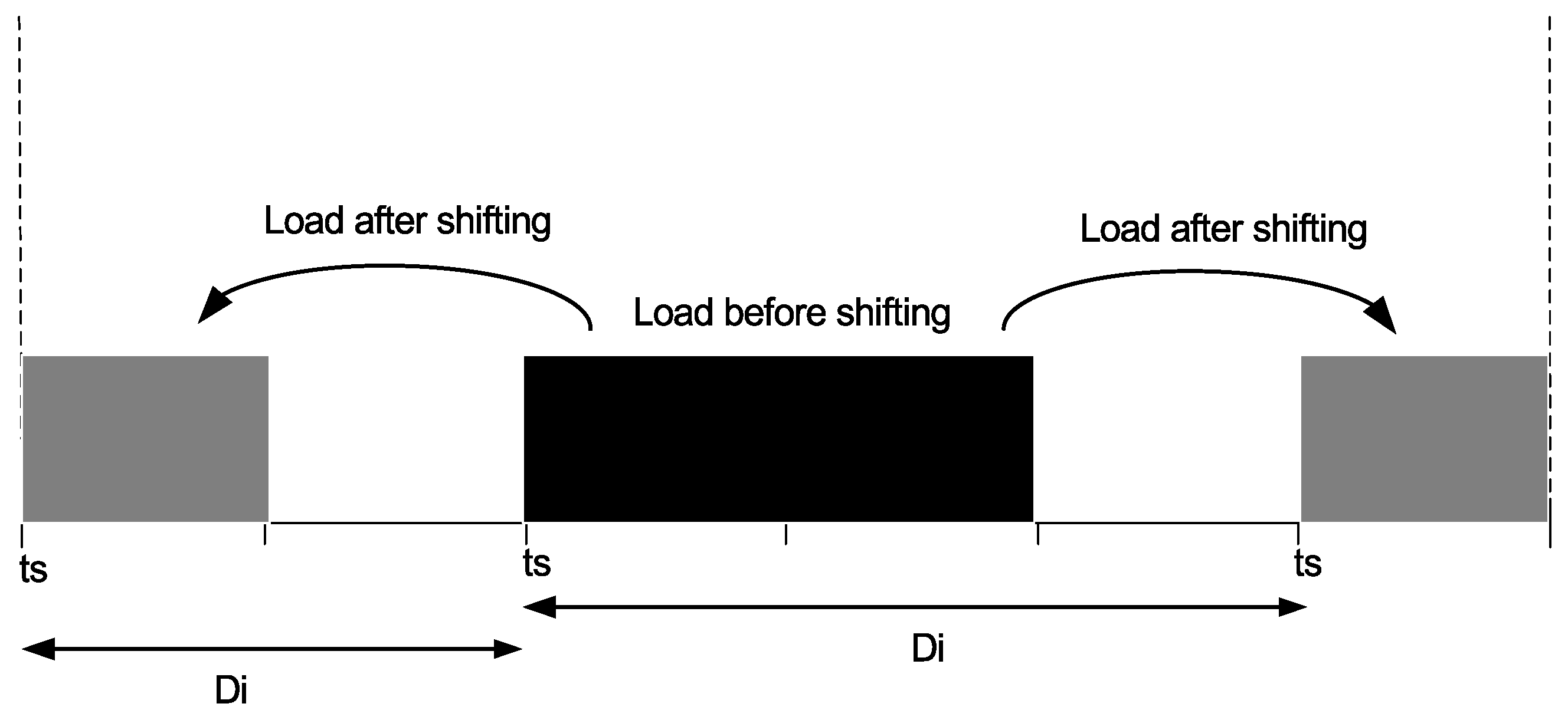
In load scheduling problems,
el and
iel appliances (
Section 3.3.3 and
Section 3.3.4) are shifted from on-peak hours to off-peak hours while aiming electricity cost reduction (
Figure 4). In this case, users may face surplus delay in terms of appliance waiting time with high probability of exceeding a bearable limit which ultimately affects user comfort. To avoid user frustration, our objective here is to reduce appliance waiting time along with electricity cost reduction of the
el and
iel appliance. For this purpose, we formulate user frustration as a function of appliance average waiting time which is calculated as [
21]:
where,
is appliance delay due to appliance shifting which is difference between appliance
and
time. The scheduling algorithm adjusts the appliances before or after specified time in response to electricity price and user preferences. The appliance waiting time can be negative (left hand side of
Figure 4) if appliance is scheduled before specified time and vice versa. The maximum waiting time that an appliance can bear is calculated as follows:
where,
is the maximum permissible delay of any appliance. User frustration increases if we increase
. In worst case, the user frustration is maximum, when
is equal to
. The user frustration
is calculated as follows:
3.3. Types of Appliances
Within the house, each appliance consumes variable amount of energy based on energy demand and customer preferences. So, we group these appliances based on user comfort maximization and electricity cost reduction perspectives. These categorizations are only used to analyze the energy consumption behaviours based on associated constraints and its impact on end user comfort. We have selected non overlapping appliances (having unique set of constraints) in the refined version of manuscript. Thus, the on/off schedules are no longer ambiguous.
3.3.1. Appliances
Typically, the working of tc appliances is controlled by CPCT. In this paper, the appliances are controlled not only by considering thermal constraints but also human occupancy. Along with other operational constraints, the working of these appliances also depends on thermal constraint such as temperature. HVAC and refrigerator are examples of appliances that belong to tc category and appliances other than these two which meet the given criteria can also be included in this category. The details of mathematical models and working of tc controlled appliances are given as follows:
HVAC
Energy consumption of HVAC depends upon two factors: (i) total number of occupants in the room and; (ii) temperature. Here, we aim to minimize electricity cost of the consumers while taking into consideration their comfort level. In most of the traditional energy management techniques, appliances are scheduled based on low electricity cost which overshadow comfort. To maintain room temperature within specified limits [
,
], HVAC consumes total energy
as follows [
29]:
The occupancy value is calculated as:
If the temperature is within given limits, the value of
variable is 0. Otherwise, its value is equal to 1. The
variable is used for simulation purpose which is denoted as follows:
where:
–: total energy consumed by HVAC
–: total number of time slots which are 24
– : minimum temperature of a room
–: maximum temperature of a room
–: energy consumed by HVAC when there is no occupant in the room
–: energy consumed by HVAC when there are occupants in the room
–: shows the state of person presence in the room [0, 1]
–: appliance on/off status
Equation (5a) represents that room temperature varies within specified limits, (20–26 ). As temperature deviates from given set points, HVAC needs more energy to keep temperature within given limits and vice versa. So, the energy consumption range in the presence and absence of occupant(s) is represented by Equation (5b). Energy consumption of HVAC is varied with the number of occupants in the room. Equation (5c) shows the presence of occupant(s), such that energy consumption of HVAC is times increased. In conclusion, these constraints show that temperature has direct impact on the energy consumption of HVAC.
Refrigerator
We aim to minimize the daily monitory expense related to the power consumption of the refrigerator while considering thermal constraints of the refrigerator. Inside temperature of the refrigerator must be within temperature range of [
,
]. To keep refrigerator’s inside temperature within acceptable limits, total number of door open attempts and duration must be at minimum because these attempts and the associated duration directly affect energy consumption. The energy consumption of refrigerator is given as [
29]:
where:
–: total energy consumed by refrigerator
–: maximum temperature limit of a refrigerator
–: minimum temperature limit of a refrigerator
Here the is equal to the sum of energy consumption in standby , compressor , with door open attempts and with temperature , respectively. Refrigerator consumes times more energy on each door open attempt. Similarly, refrigerator consumes times more energy with outside temperature variations. It means, energy consumption of a refrigerator depends upon its temperature variations. Equation (6a) represents the internal temperature bounds of a refrigerator.
3.3.2. Appliances
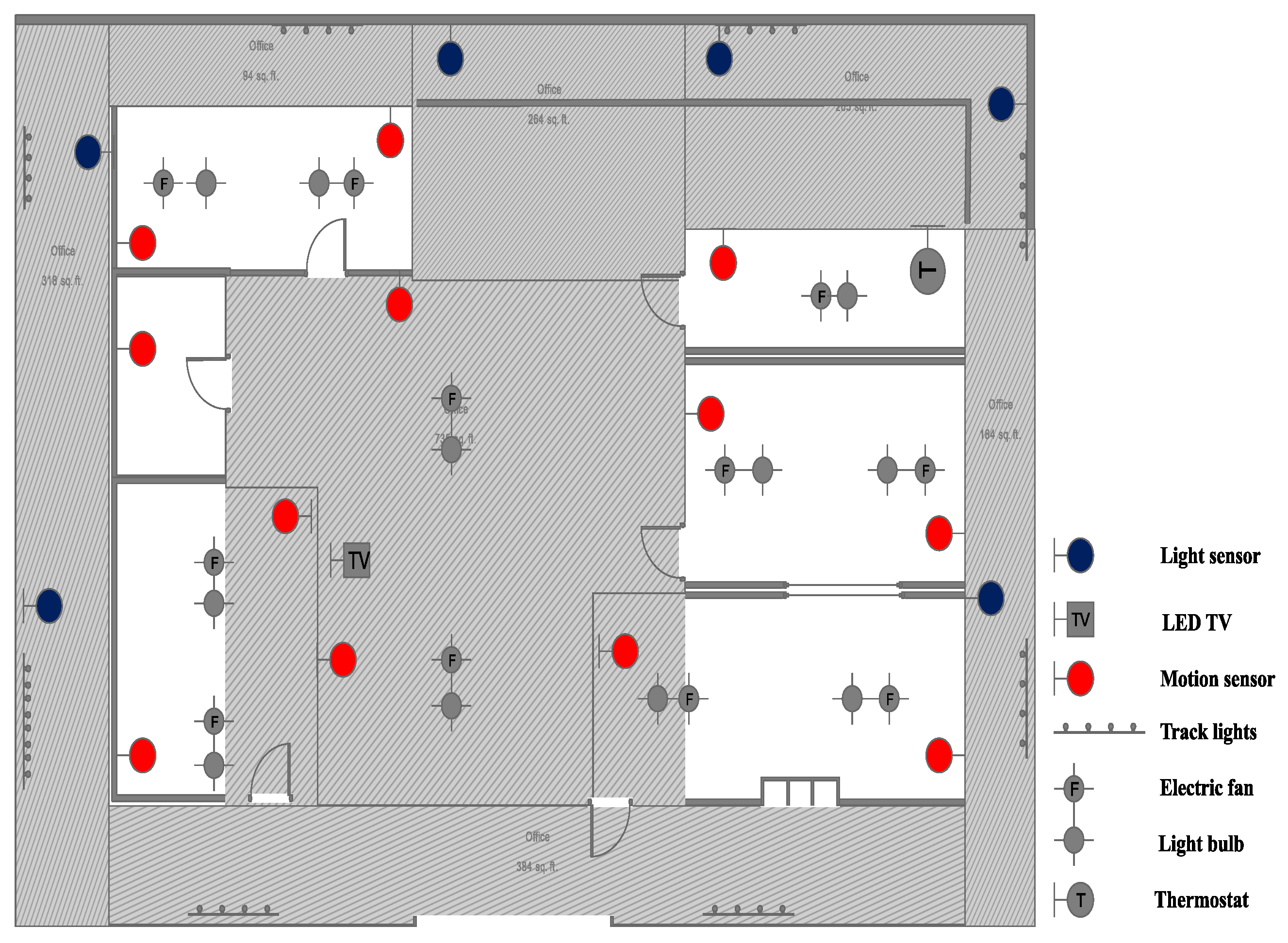
These types of appliances are turned on or off on the basis of human occupancy. For this purpose, we assume that different sensors are deployed in the room in order to detect human presence (
Section 5). When any sensor detects human presence, their respective appliance(s) are turned on and energy consumption is calculated. By using human presence mechanism, unnecessary appliances can be turned off to reduce uneven energy consumption. Moreover, any appliance which meets the
ua criteria, can be considered in this category. Total energy consumption of
ua appliances can be calculated as given in [
29]:
where:
where:
Equation (7a) shows that total energy consumption of ua appliances depends upon parameter. The appliances associated with these sensors remain on or off based on the values of these sensors.
3.3.3. Appliances
These are fixed energy consumption appliances, however, these are interruptible whose working can be scheduled throughout the time interval. In order to save electricity cost, these appliances are scheduled in low pricing hours. Total energy consumption of these types of appliances is calculated by using the following equation:
el appliances perform their tasks under the following constraints:
where:
–: appliance duty cycles (total operating hours)
–: energy consumption capacity limit used for PAR reduction
–: total time in which appliance can be scheduled (appliance scheduling horizon)
–: appliance total waiting time occurs due to rescheduling
–: appliance unscheduled starting time initially set by users
–: appliance scheduled starting time set by energy scheduler
Equation (8a) represents that unscheduled and scheduled are equal. Total energy consumption of el appliances is within energy constraints which is given in Equation (8b). Whereas, Equation (8c) represents the scheduling horizon of el appliances. As these types of appliances are interruptible so their operating time may vary in scheduling horizon. Equations (8c, 8d) represent the appliance waiting time and on/off status, respectively.
3.3.4. Appliances
These types of appliances are interruptible and continue their operation once turned on. User can not compromise on comfort, so these appliances are turned on when electricity price is low and complete their duty cycle without interruption. Energy consumption of these types of appliances is calculated by using the following equation:
The associated constraints for
iel appliances are listed as follows:
Equation (9a) represents that appliance unscheduled must be equal to scheduled . Equation (9b) shows that total energy consumption of iel appliances must not exceed . Because these appliances are uninterruptible, so they have continuous after scheduling. Total scheduling horizon of these appliances is given in Equation (9c). Waiting time of these appliances is not more than 3 h as we impose this limit. Equation (9d) represents the total waiting time. Appliances on/off status is represented by Equation (9e).
3.3.5. r Appliances
We consider that these appliances are continuously running during whole day. So, these appliances do not take part in DR programs and thus can not be scheduled. Energy consumption of
r appliances is calculated by using the following equation:
where,
is total energy generated by local generator,
is energy consumption of
r appliances and
is total energy consumption of
r appliances, respectively.
3.3.6. Total Energy Consumption
The total energy consumption
of all types of appliances including
el,
iel,
r,
ua, and
tc, is calculated as follows:
The daily total electricity cost
of these appliances is given as:
Equation (
13) shows that
is equal to the electricity taken from grid. The second part of Equation (
13)
denotes the energy demand of
r appliances is fulfilled through microgrid model (
Section 3.1). The final cost minimization objective function is given as:
3.4. Peak to Average Ratio Reduction
Along with electricity price, PAR reduction of the system is also taken into consideration to increase the stability of the grid. For this purpose, we introduce energy consumption capacity limit in the optimization problem. PAR can be calculated by using the following expressions:
where
is maximum peak and
is average peaks.
By reducing PAR, we can achieve system stability and increase spinning reserves capacity of the power system. Moreover, reduction in peak load demand leads to reduction in peak power plant cost and transmission losses.
Note: When a person is in a room, he/she would like that the temperature is already within the limits, or close to them: if the HVAC is off whenever nobody is in the room, the temperature might get very far from the limits, causing an unpleasant environment most of the times someone gets in the room. However, for this purpose, we need to predict human behaviors based upon their daily, weekly, or monthly schedules. Then based on these behaviors, we can predict when a person will probably enter the room/house and schedule HVAC, accordingly. This might increase total energy consumption as behaviors and schedules are dynamic but at the same time increasing end user comfort in terms of balanced room temperature. In conclusion, advanced/intelligent prediction techniques are needed, which demand research work beyond the scope of this paper. For the sake of simplicity in implementation, this research work carries out implementation with the assumption of uniformly distributed person arrival to the room.
4. Genetic Algorithm Based Energy Management Algorithms
Typical scheduling optimization problems have discrete, non-linear and highly constrained search space which make desired solutions very difficult to find. Various mathematical optimization techniques are being used to solve these types of problems and it is impossible that single algorithm gives best optimal solution to different optimization problem. Among these, EAs are extensively used for solving such types of complex optimization problems due to fast convergence and ability to deal with different dynamics of the problems. Furthermore, these algorithms are efficient in providing optimal solutions when other mathematical optimization algorithms fail to provide [
30]. Therefore, we use GA to solve the complex energy optimization and appliance scheduling problem.
There are seven major steps of GA: initialization of parameters, fitness evaluation, selection, crossover, mutation, elitism and generation of new population. The details of these steps are given as follows:
Initial Population: In first step, random population which consists of candidate solution (chromosomes) is initialized. The initial population is in
nxm matrix form, where
m and
n represent population size and total number of appliances, respectively. The matrix
is written as follows:
Fitness Evaluation: In this step, fitness of randomly initialized population is evaluated such that if chromosome (m = total no. of appliances) is [1 0 1 1 1 0], it means appliances 1, 3–5 are on. We then calculate cumulative power and multiply it with electricity price to calculate energy consumption cost. This process continues until the evaluation of population’s fitness. This process gives an optimal pattern of household appliances at time slot t whose electricity cost is low.
Selection: At the start of the algorithm, random population is initialized only once. In the next generation, new population is generated through mutation and crossover operators. For this purpose, a random pair form random population is selected to form new population. We use tournament based selection procedure to select a random pair.
Cross over and Mutation: After the selection of random pair, new population of chromosomes is produced by using mutation and crossover operators. There have been different methods of crossover and mutation, and we use binary mutation and single point crossover methods. Convergence of GA depends on mutation and crossover rate. Higher crossover means faster convergence. On the other hand, high mutation rate may diverge optimal solution, which means slow convergence.
Elitism: Sometimes, near optimal solution is found at the start of algorithm but after mutation and crossover, it may be lost. So, elitism is used to save this solution for evaluation purpose. As we discussed earlier that GA has comparatively faster convergence rate where the convergence mainly depends upon crossover and mutation probability. Higher crossover probability results faster convergence and higher mutation probability results less optimal solution and vice versa. Moreover, improper adjustment of these parameters may result premature convergence of the algorithm. However, in some cases the best optimal solution can be found earlier and after that crossover and mutation may variate this solution. So, elitism mechanism is used to keep the optimal solution in the next step from one generation to another to get final optimal solution. The parameters based on which the optimal schedules of different appliances are generated are shown in
Table 2. Based on RTP signal, energy demand and user requirements, GA generates the optimal patterns of all appliances in each time slot. For example, if we have six appliances, six bit binary pattern (011001) is generated where 0 shows off and 1 shows on state of appliances. In each time slot, this process repeats to obtain optimal patterns because electricity prices vary based on energy demand of the appliances and user preferences.
4.1. Complexity of Genetic Algorithm
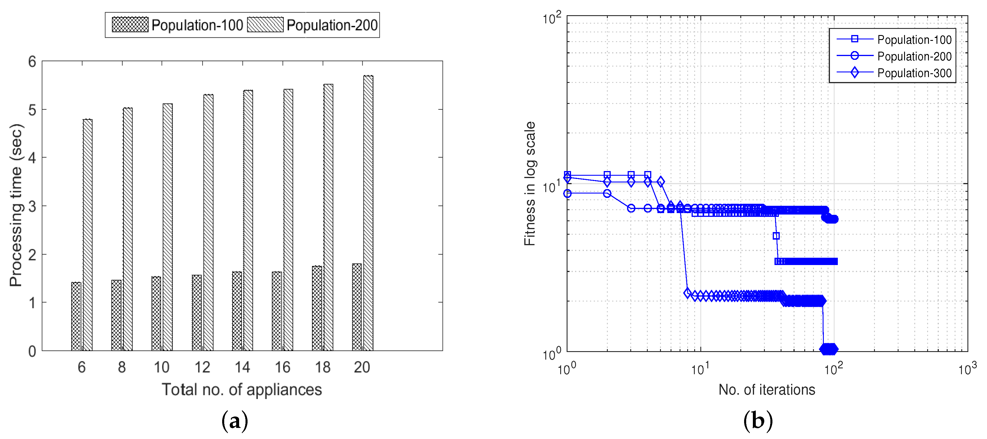
In GA implementation, representation of solution is vital to its convergence and processing time (speed). GA algorithm produces the best solution by evaluating the initial random population. The size of initial population usually depends on the nature of the problem. The algorithm takes more processing time to evaluate the fitness of all individuals for large population size and vice versa.
Figure 5 shows the analysis of processing time and fitness function w.r.t population size and total number of appliances. It is clear from
Figure 5a that processing time increases by increasing total number of appliances in time
t. It is also shown that algorithm takes more processing when initial population size is large as compared to small population size. This is because the algorithm evaluates
matrix which can take more processing time while taking into consideration all constraints (Equations (9a–9e)). In
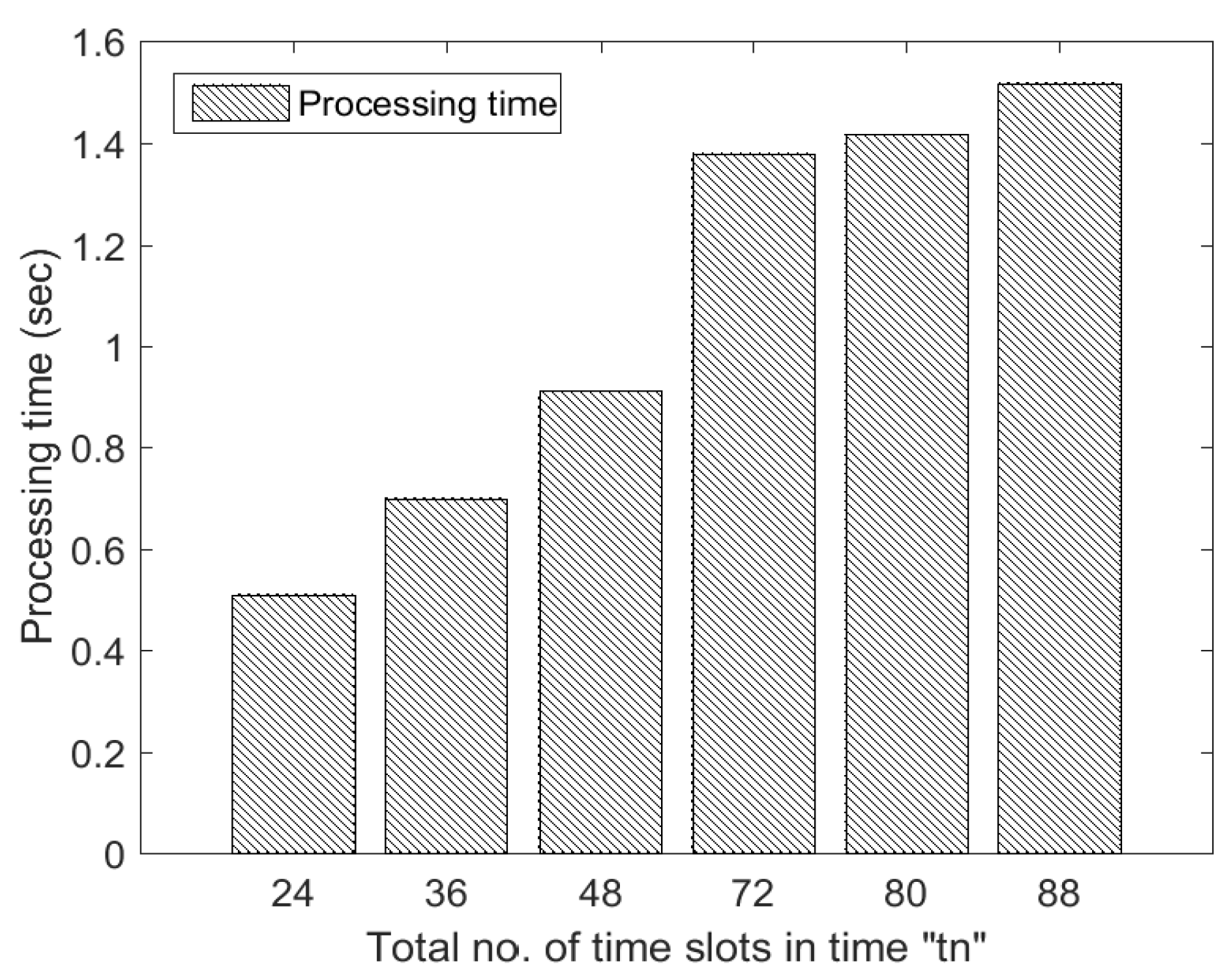
Figure 6, processing time of GA in terms of total number of time slots has been shown. It is clear from the figure that processing time (convergence time) increases as we increase the total number of time slots during time
t and vice versa. This is due to the fact that algorithm needs more time to find optimal time slots when total number of time slots are increased. In the proposed work, we use 24 and 48 time slots for simulation purpose to evaluate the performance of GA in terms of convergence, processing time and optimal solution
Figure 5 and
Figure 6. The proposed algorithm has the capability to schedule home appliances considering any number of time slots, but at the cost of more processing time. In conclusion, complexity of the proposed algorithm increases as we increase the total number of appliances, time slots and initial population size.
5. Simulations and Results
In this section, we discuss the simulation results and assess the performance of the proposed energy management algorithms in terms of energy consumption, electricity cost savings and thermal comfort of the consumer. Different types of appliances, i.e.,
tc,
ua,
el,
iel,
r, having variable energy demand and operating time have been considered in this work. The working of
tc appliances is controlled by taking into consideration human occupancies and thermal constraints. The
ua appliances are turned on only when any person is present in the room. For this purpose, we assumed different sensors placed in the room which detect human motion/presence and provide signal to EMC [
31]. Based on this information, EMC decides to turn that particular appliance on or off. The
el appliances are those which can be scheduled throughout the day. Moreover, these appliances are interruptible in nature and EMC schedules these appliances for cost reduction perspective without violating
. On the other hand, the
iel appliances are scheduleable but non-interruptible in nature. Once these appliances are turned on, they will complete their working hours. At the end, the energy demand of
r appliances is fulfilled through local generation because these are continuously running appliances as discussed in
Section 3. The details about the appliances used in these categories and simulation parameters are given in
Table 1,
Table 2,
Table 3,
Table 4,
Table 5 and
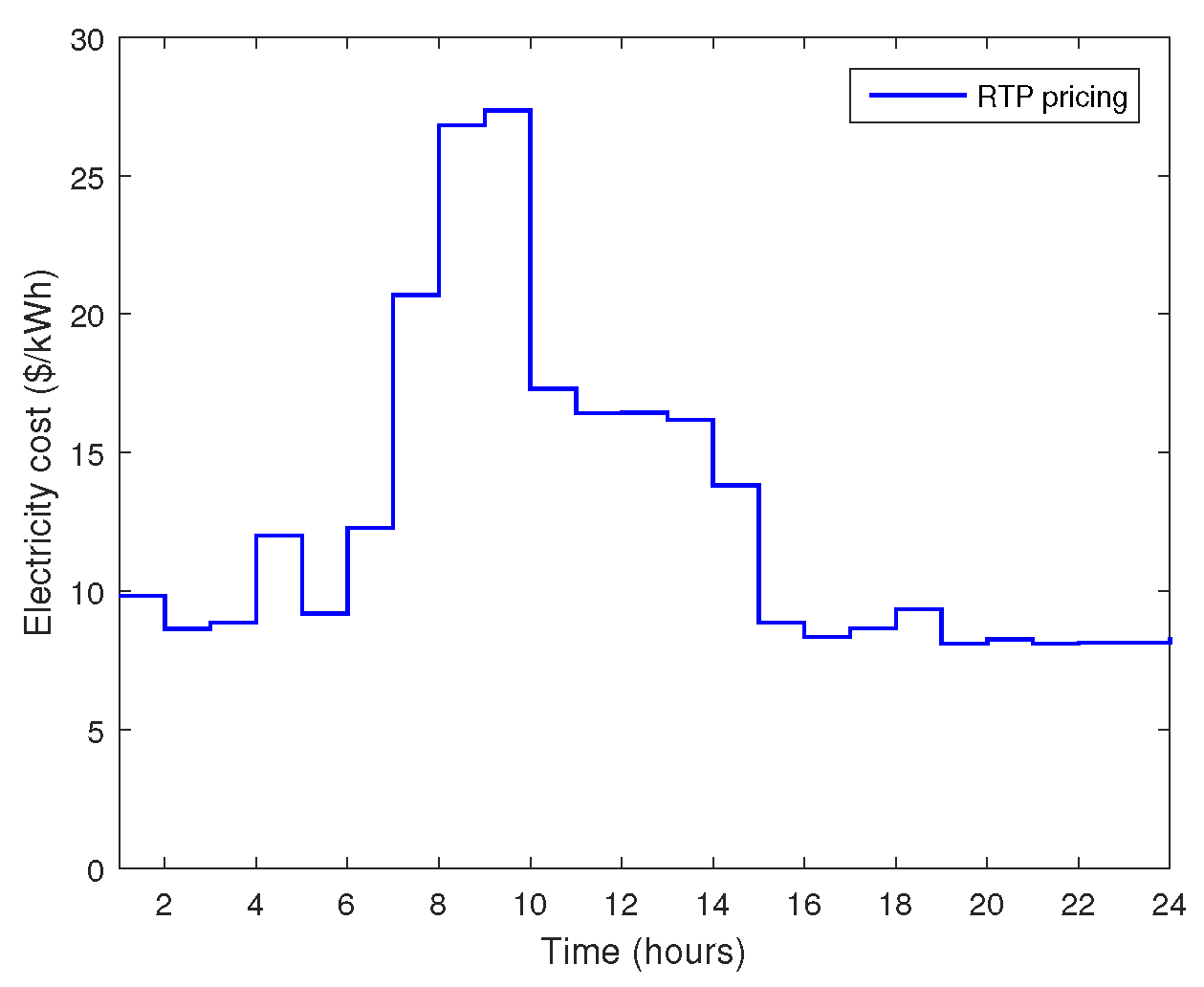
Table 6, respectively. The RTP signal is directly obtained via smart meter which later on is utilized by EMC for appliance scheduling and controlling (
Figure 7, [
32]).
| Algorithm 1 Pseudo code of the proposed algorithms for tc and ua appliances |
- 1:
Required population size, max. generations, N, Temperature range, , , , , . - 2:
Initialize random population which represents the patterns of appliances. - 3:
for t=1:tn do - 4:
for i=1:popsize do - 5:
Evaluate fitness function. - 6:
F= - 7:
—–For HVAC System———- - 8:
if then - 9:
- 10:
if then - 11:
- 12:
end if - 13:
if then - 14:
- 15:
end if - 16:
else - 17:
- 18:
end if - 19:
—–For refrigerator———- - 20:
- 21:
if then - 22:
- 23:
if then - 24:
- 25:
end if - 26:
if then - 27:
- 28:
end if - 29:
if then - 30:
- 31:
end if - 32:
—–For appliances———- - 33:
if then - 34:
- 35:
if then - 36:
- 37:
- 38:
- 39:
- 40:
end if - 41:
if then - 42:
- 43:
- 44:
- 45:
- 46:
end if - 47:
if then - 48:
- 49:
- 50:
- 51:
- 52:
end if - 53:
end if - 54:
else - 55:
end if - 56:
end for - 57:
end for - 58:
if then - 59:
- 60:
- 61:
end if - 62:
end if - 63:
else - 64:
- 65:
end if - 66:
end for - 67:
Generate new population. - 68:
Select crossover pair - 69:
if then - 70:
- 71:
end if - 72:
- 73:
if then - 74:
- 75:
end if - 76:
popnew(popsize,N) - 77:
end for
|
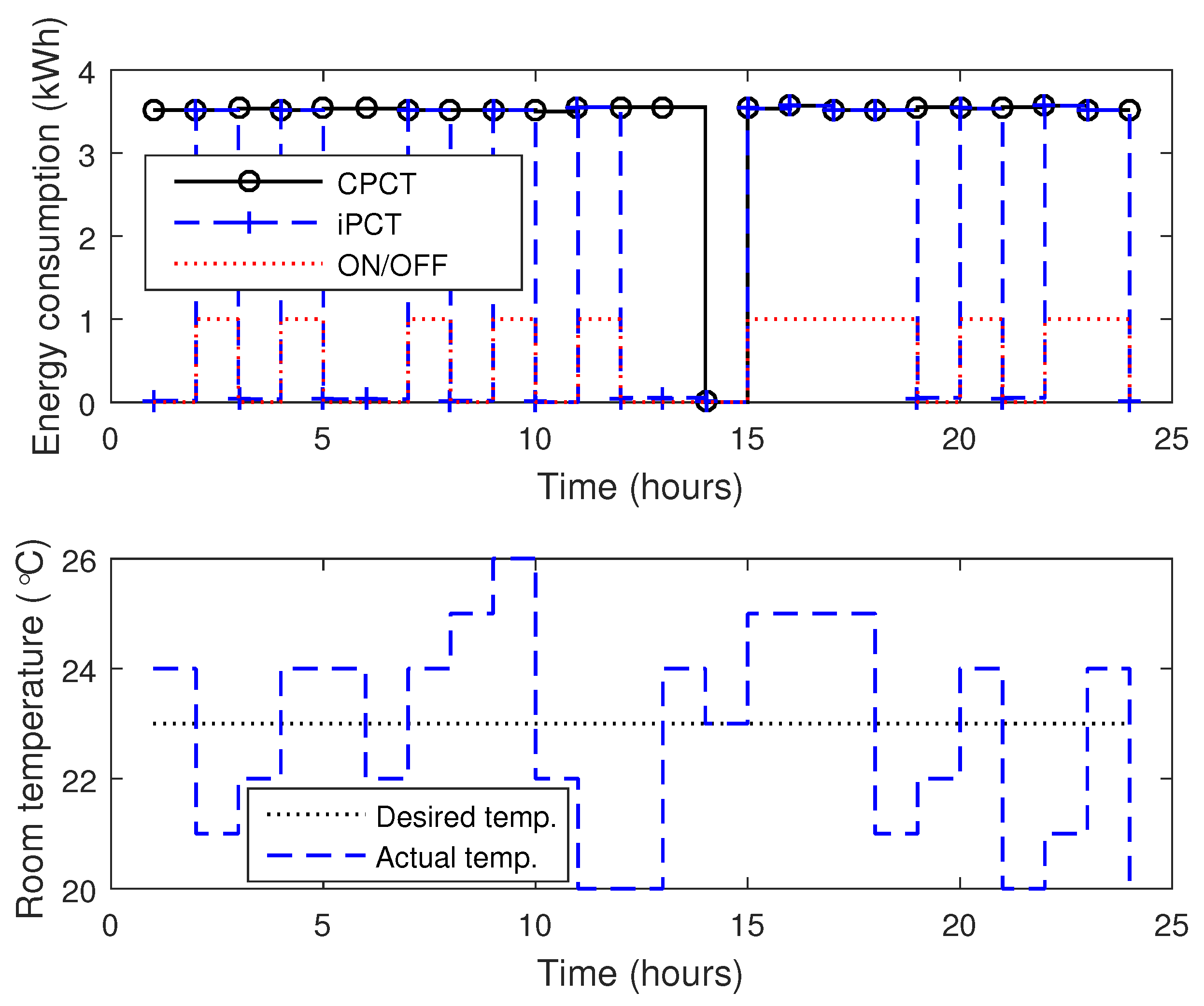
Figure 8 illustrates the energy consumption of HVAC in case of CPCT and iPCT. Using CPCT, HVAC turns on when indoor temperature falls below the threshold temperature
,
and turns off when temperature level is maintained in the room
. Turning on HVAC without taking into consideration the human occupancy may increase the energy consumption leading to high electricity cost. To enhance the appliance utility, the proposed algorithm considers all these factors (temperature and occupancy) and maintains the desired room temperature. It is clear from
Figure 8 that when there is no occupant in the room
and
(red dotted line), EMC sends turn off signal to the iPCT. For simplicity, only occupants presence has been shown in
Figure 8a based on which HVAC turns on or off. From
and
, there is again no occupant in the room and iPCT turns off the HVAC according to (
Section 3.3.1). In case of CPCT, HVAC is turned on during time slots
and
on the basis of temperature difference only (
Figure 8). Although, there is no occupant found in these time slots which is an important reason of uneven energy wastage. During time slot
, both CPCT and iPCT turn off HVAC because there is no occupant in the room and temperature is within desired limit. From above results, it is clear that iPCT is more efficient in handling appliance working as compared to CPCT.
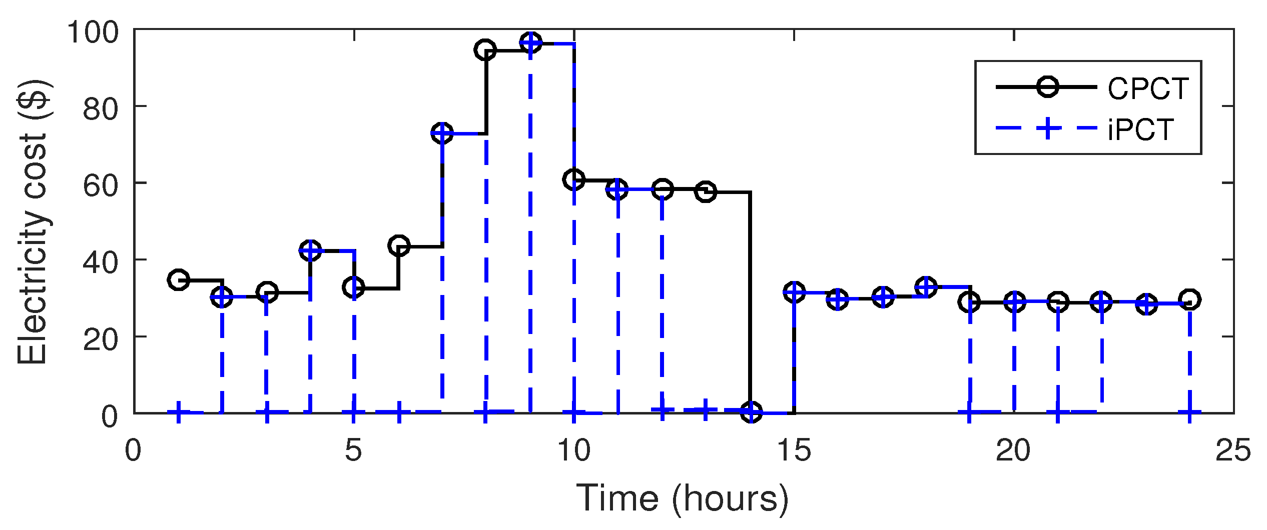
Figure 9 shows the resultant electricity cost of HVAC.
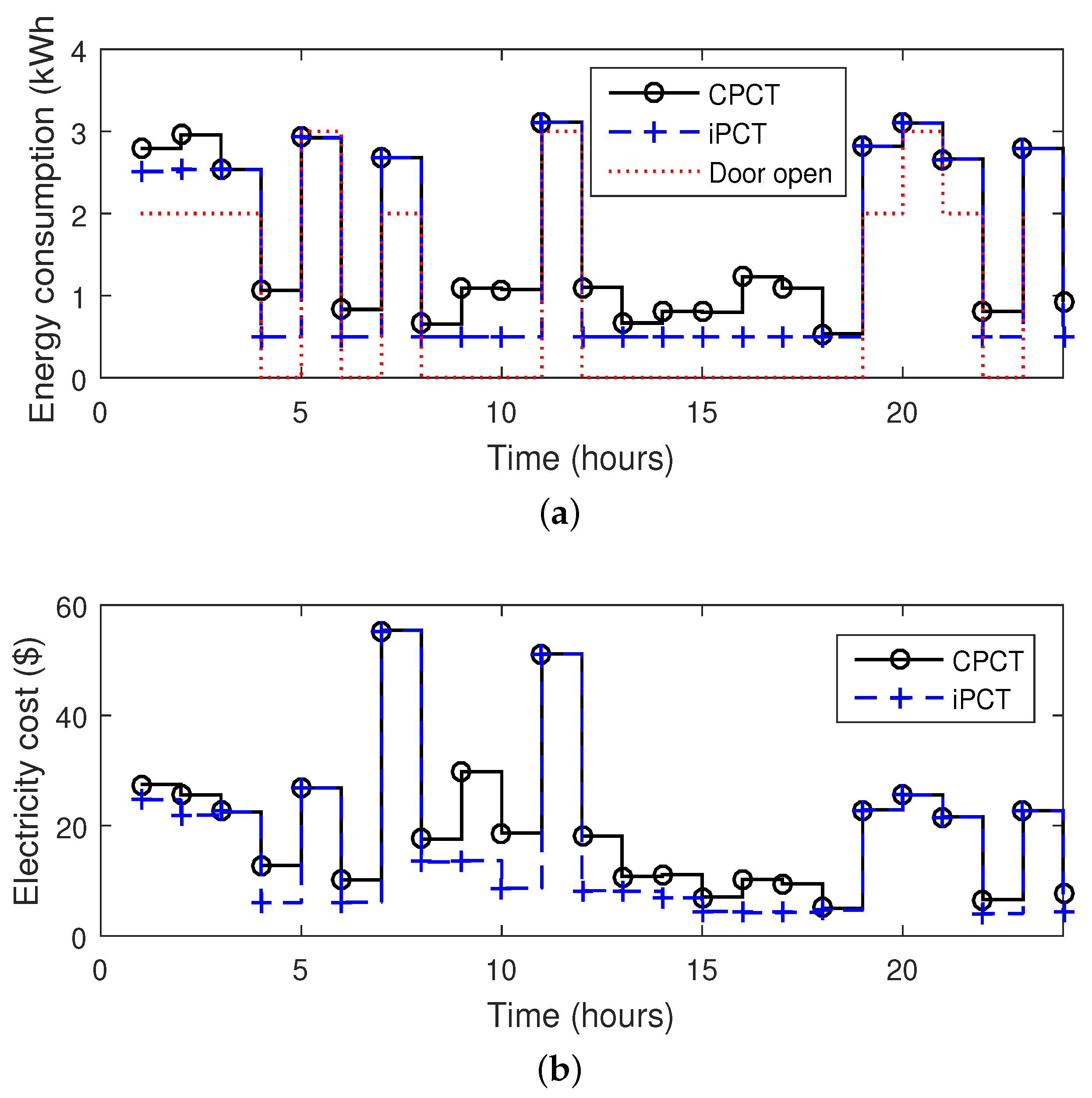
In case of refrigerator, energy consumption depends on outside temperature variations and number of times the door is opened. The number of times the door opens in a single time slot is considered uniformly distributed random variable within the range of [0,4]. Each time when door is opened at for 12 s, additional energy of 12.4 W/h/day is consumed. It is clear that the door opening rate is directly proportional to the total duration required for user satisfaction. The iPCT turns on the refrigerator compressor only when the inside temperature exceeds . Otherwise, compressor remains off to reduce the electricity cost.
The daily energy consumption of refrigerator is shown in
Figure 10a. From
, refrigerator’s door is opened with a constant rate (2 times) based on which energy consumption is calculated. From
,
,
,
and
, refrigerator’s door is closed as shown via red dotted lines (
Figure 10a). However, energy is still consumed because the compressor needs energy to keep inside temperature within desired limit (
Figure 10b). However, the energy consumed in case of iPCT is less as compared to CPCT. Due to proper tuning of
and
variables (
Section 3.3), total energy consumption and electricity cost of refrigerator are comparatively less in case of iPCT. Using iPCT, total energy consumption of refrigerator is reduced from 40.6864 kWh to 34.53 kWh which is 15.12 % reduction. The daily electricity cost of refrigerator is reduced from 476 $ to 392 $, which is approximately 18 % reduction. These results verify that under same conditions, the proposed algorithm efficiently reduces the daily electricity cost and maintains the internal temperature of refrigerator within desired range. The parameters and temperature set points used to model the optimization problem of a refrigerator are given in
Table 5.
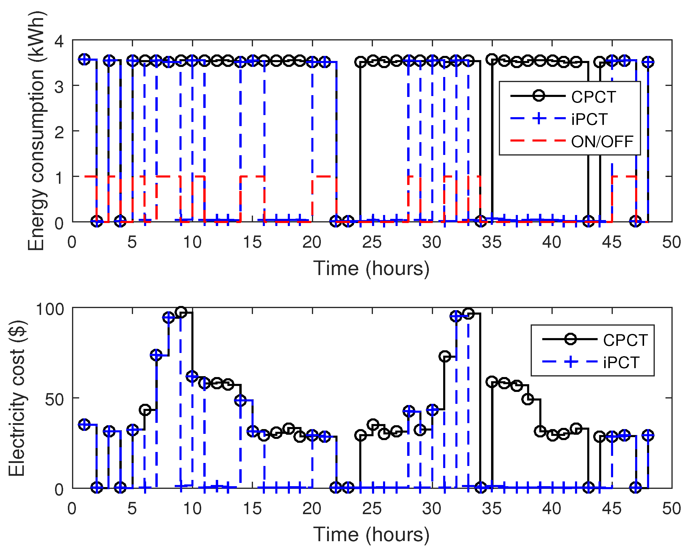
In order to visualize the impact of short time slot on energy management system and its stability, the proposed algorithms of HVAC and refrigerator are tested for
t = 30 min time window. This section explains the energy consumption and electricity cost of HVAC and refrigerator in relation to three number of parameters: (i) total number of door open attempts; (ii) temperature variations; (iii)
t = 30 min time slot. Considering CPCT, HVAC turns on based on temperature variations. While in case of iPCT, HVAC turns on based on temperature variations and total number of persons in the room. It is clear from
Figure 11 that in case of iPCT, HVAC frequently turns on and off based on total number of persons present in the room. In
Figure 12, total energy consumption and electricity cost of refrigerator is shown which is based upon total number of door open attempts (
Section 3.3.1 (Refrigerator)). It is clear that during time slots
, refrigerator’s door is closed and resultant energy consumption is zero and vice verse. The total electricity cost savings of HVAC and refrigerator are 52% and 63.47%, respectively.
Discussion:
Figure 11 and
Figure 12 show that the proposed algorithms have the capability to manage the loads even if time window is less than 1 h. Although, the energy management system works efficiently however there might be some complexities when using the small time window: (i) processing time can be increased; (ii) system complexities may increase because it is comparatively more complex to handle short time windows; (iii) it is very difficult for utilities to design real time DR programs based on small time slots. The reason behind this is the large amount of communication data exchanged between utilities and consumers. This is the main reason that most utilities are heavily relying on time of use (TOU) and day ahead pricing (DAP) schemes. Most importantly, the system with short time slot is efficient because
ua appliances can be turned off based on human occupancy.
On the other hand,
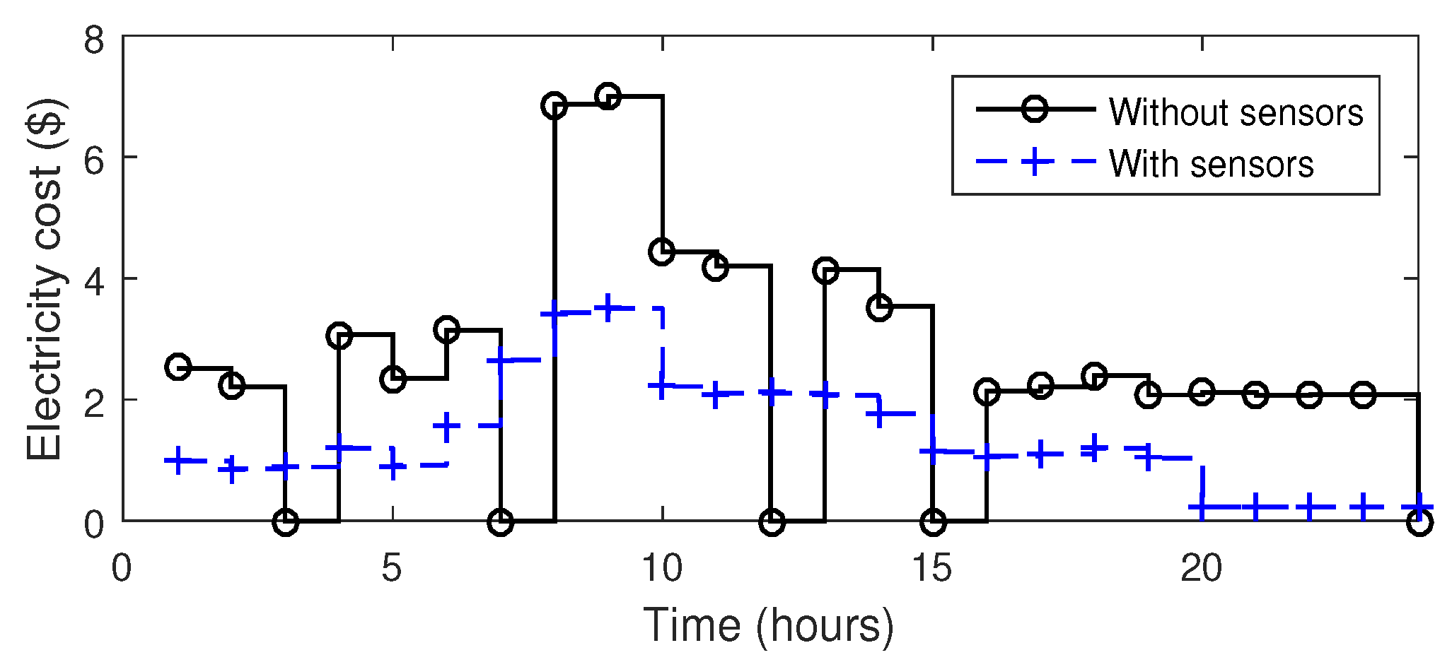
ua appliances are scheduled on the basis of occupancy data. EMC turns on fans and lights if any person is present in the room. If
= 0, it means that person is not present in the room and the associated appliance is off and vice versa. This mechanism reduces unnecessary energy consumption of
ua appliances and thus efficiently utilizes the energy. From
Figure 13, it is clear that energy consumption of
ua appliances is almost half when occupancy and light sensors are not used. The energy consumption is reduced from 4.86 kWh to 2.43 kWh in a single day which is almost 50% saving. The daily electricity cost of
ua appliances is shown in
Figure 14 and the working of HVAC, refrigerator and
ua appliances is explained in
Figure 15.
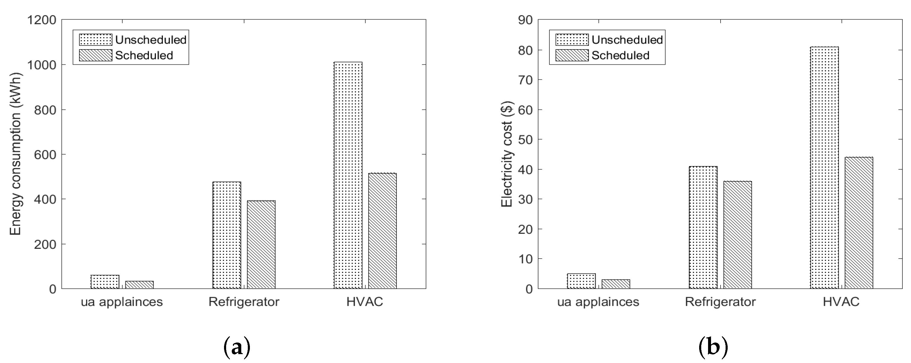
The daily energy consumption and electricity cost of
tc appliances (HVAC and refrigerator) and
ua appliances (fans and lights) are shown in
Figure 16. In case of
ua,
tc appliances, the daily electricity cost is reduced by 49.01% and 45.67%, respectively. This is due to the fact that before turning
ua,
tc appliances on, EMC checks the presence of person(s) in the room as described in (
Section 3.3.1 and
Section 3.3.2). In traditional scheduling schemes, the working of HVAC is controlled on the basis of temperature difference only [
22]. Furthermore, the electricity cost reduction of refrigerator is approximately 18% which shows that minimization of the opening duration of refrigerator’s door leads to significant energy saving. It is also shown that our algorithm makes the CPCT more intelligent and operates at optimal cost while considering the HVAC constraints.
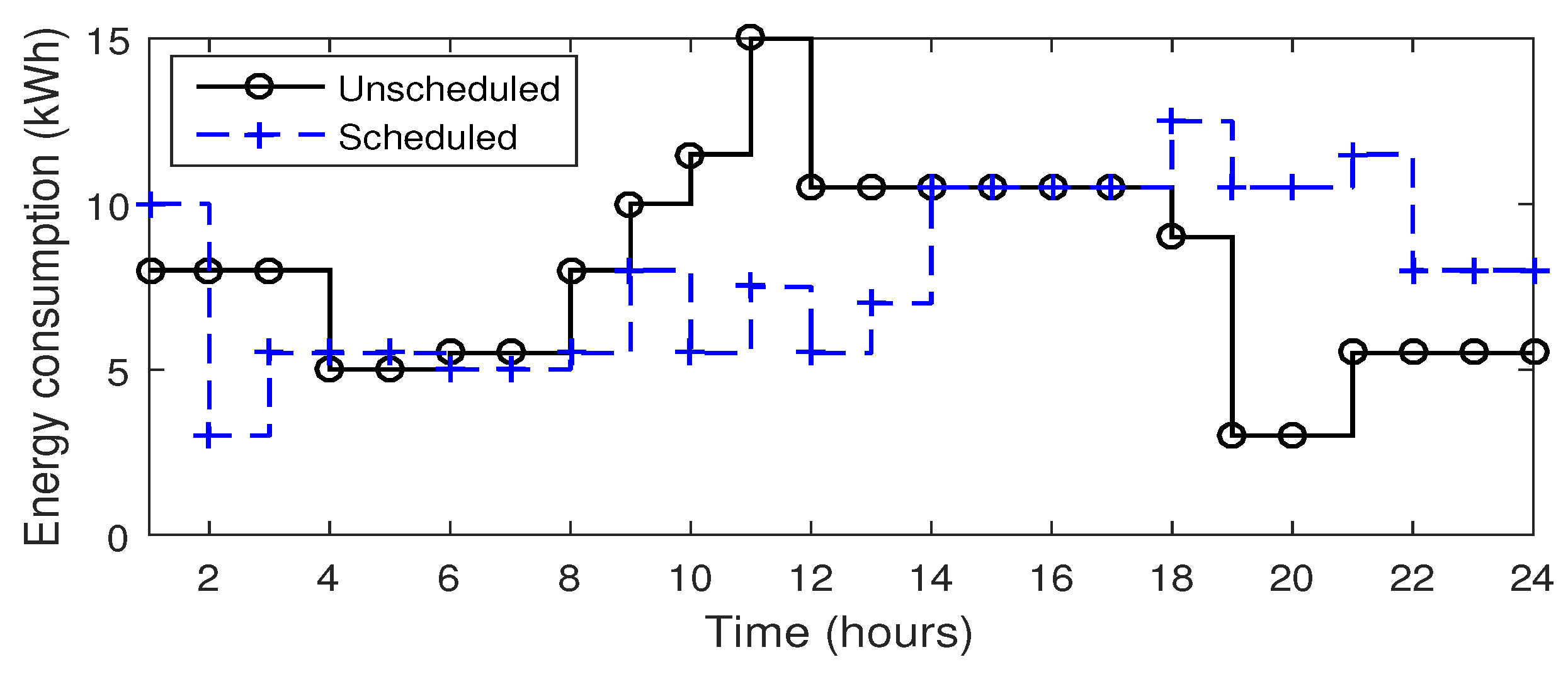
Figure 17 illustrates the energy consumption of
el and
iel and
r appliances. It is clear that the proposed algorithm efficiently schedules the appliances according to electricity prices and user preferences. The EMC schedules maximum appliances in low price hours
and
, however it is also illustrated that some of the appliances are still running in critical time slots (i.e.,
). There are two main reasons behind this operation; (1) due to user comfort, because users do not want to compromise on their comfort; (2) due to total
constraint. One of the possible drawbacks of scheduling more appliances in low price hours is the possibility of high peaks on gird. In this situation, the proposed algorithm should be capable enough in handling high peak problem. So, we significantly avoid this problem by imposing knapsack capacity limit constraint Equation (9b). In general, the consumers are not the only stake holders in DSM programs, both utility and consumer can get equal benefits. This reduction in peak load demand decreases the PAR which improves the stability and the utilization factor of the grid.
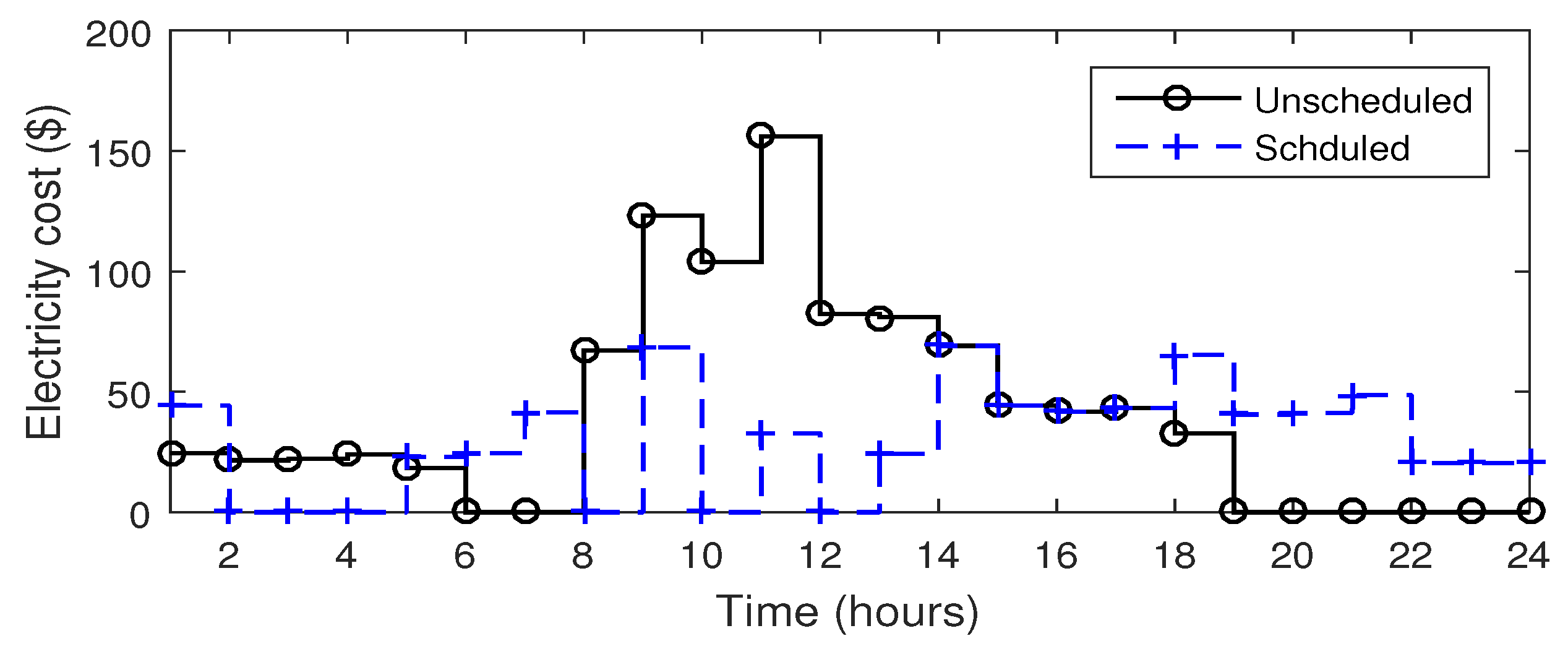
In
Figure 18, the hourly electricity cost of
el,
iel and
r appliances is shown. It is clear from the figure that from time slot
there are high peak hours. The proposed algorithm efficiently shifts the controllable appliances in time slots
to reduce the electricity cost (due to constraints 8a-8e and 9a-9e). The
r appliances are still operated on diesel power generator (
Section 3.1, their fuel cost is given in
Table 7). This is because that the generation cost of microgrid is still less than the cost of utility. Therefore, it is feasible to operate
r appliances on generator to minimize the electricity cost and user frustration. The total electricity cost is high due to more energy consumed by
iel appliances in these time slots. Another major reason is uninterruptible nature of these appliances. On the other hand,
el appliances are interruptable and can be scheduled throughout the day (
Section 3.3.3,
Figure 19). Therefore, EMC schedules these appliances in low electricity time slots (i.e.,
,
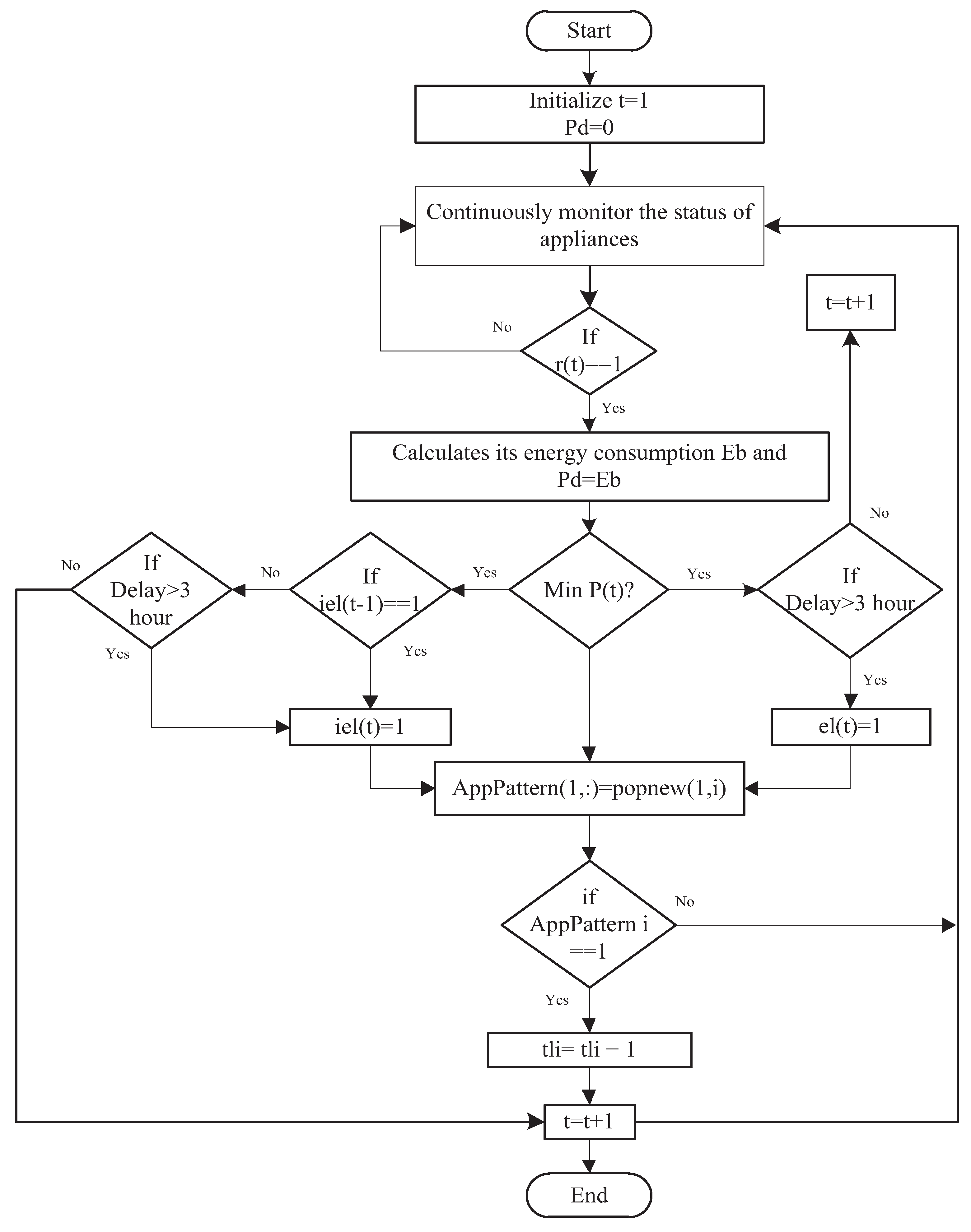
). Regarding PAR, it is reduced by 22.77% using power capacity limit Equation (9b) which increases the efficiency and stability of grid. The peak load demand without the proposed algorithm is 16.5 kW, whereas in case of proposed algorithm the peak load demand reduced to 14.5 kW. This reduction in peak load demand reduces the total generation cost of peak power plants. Furthermore, the reduction in peak load demand and PAR reduces the line losses and improves the efficiency of grid. The steps involved in the controlling of
el and
iel appliances are shown in algorithm 2.
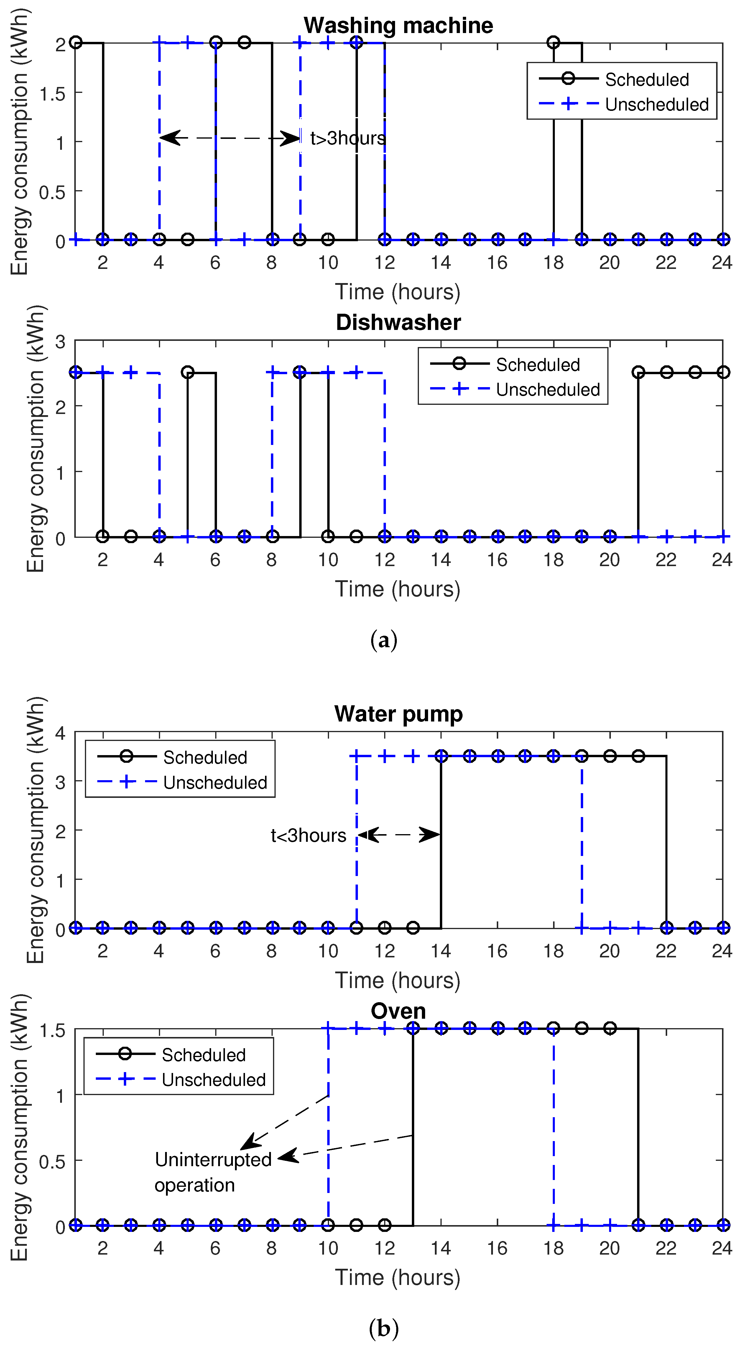
In
Figure 20a, individual energy consumption patterns of
el appliances which can be interrupted during their working cycles is shown. The
el appliances have an interruptible nature and we can turn on/off where needed to reduce the electricity cost and PAR. When interrupted, these appliances wait for the next time slot where the electricity price is low. This may increase the waiting time of appliances which ultimately disturb user comfort (
Section 3.2) due to comfort and cost tradeoff. Therefore, considering this tradeoff in mind, we design the algorithm which schedules the
el appliances in such a way that their total average delay is not greater than 3 time slots (e.g., maximum waiting time flexibility is considered 3 h in our case). However, users have the flexibility to set the maximum waiting time according to their own desire. For example, washing machine and dishwasher can wait because these appliances are not directly related to user comfort (
Section 3.2). To avoid the inconvenience,
iel appliances are considered un-interruptible with high priority. These appliances remain on until the completion of complete cycles once turned on. The waiting time of these types of appliances is not more than 3 h. It is clear from
Figure 20b that
iel appliance is turned on at low electricity price hours. However, once turned on can not be interrupted during their duty cycle. Moreover,
Figure 20b shows that the maximum delay of these appliances is equal to 3 h (high priority).
Figure 19 shows the working mechanism of
r,
el and
iel appliances.
| Algorithm 2 Pseudo code of the proposed algorithm for el and iel appliance |
- 1:
Required Unscheduled pattern, , population size, max. generations, N. - 2:
Initialize random population which represents the patterns of appliances. - 3:
for t=1:tn do - 4:
=0 - 5:
for i=1:popsize do - 6:
Evaluate fitness function - 7:
F= - 8:
if then - 9:
- 10:
if then - 11:
- 12:
- 13:
if then - 14:
- 15:
end if - 16:
end if - 17:
if then - 18:
- 19:
- 20:
if then - 21:
- 22:
end if - 23:
end if - 24:
else - 25:
- 26:
end if - 27:
end for - 28:
AppPattern(1,:)=popnew(1,i) - 29:
if then - 30:
- 31:
end if - 32:
Pd= - 33:
Solve minimization problem (1). Generate new population. Select crossover pair - 34:
if then - 35:
- 36:
end if - 37:
- 38:
if then - 39:
- 40:
end if - 41:
popnew(popsize,N) - 42:
end for
|
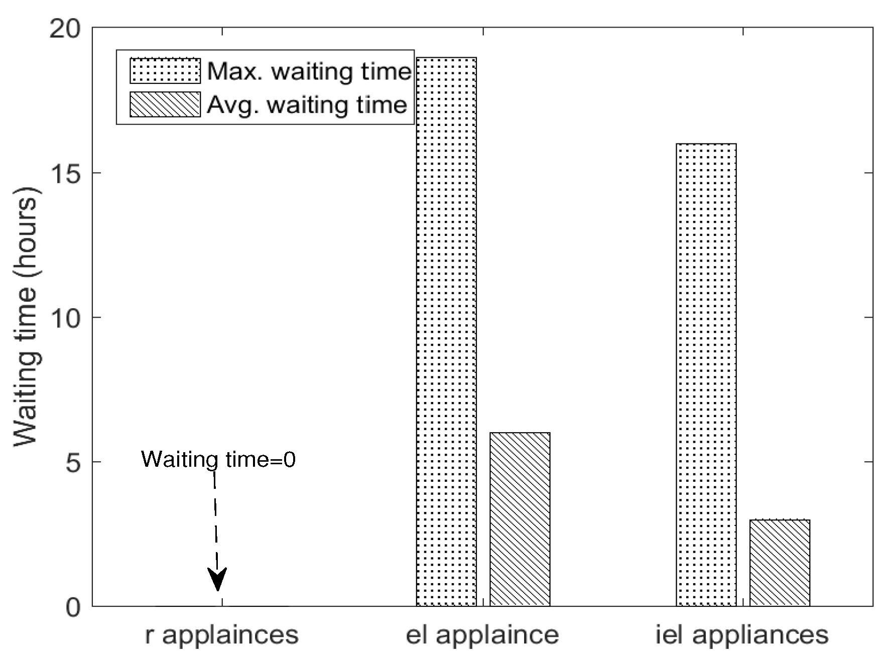
The average appliance waiting time of
r,
el and
iel appliances is shown in
Figure 21.
r appliances have zero waiting times because these appliances are served by local generation. Whereas,
el appliances have average waiting time of 6 h. From
Figure 20, it is seen that in case of dishwasher the delay exceeds 3 h.
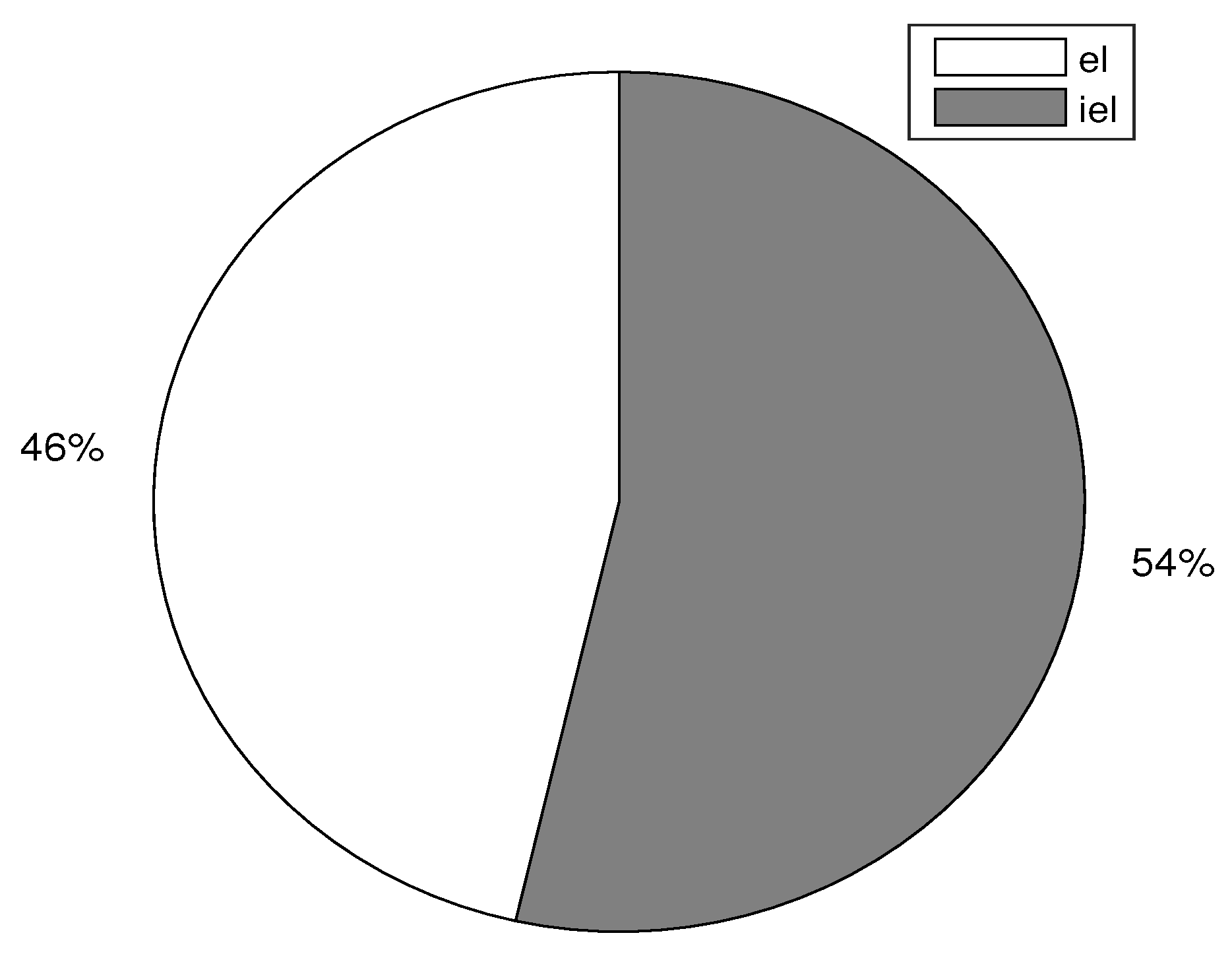
Figure 22 shows user comfort in case of
el,
iel and
r appliances. It is clear from the figure that frustration level of
r appliances is not shown because these appliances are turned on as per user demand. Moreover,
r appliances do not take part in DSM program and are not considered in optimization problem.
Figure 22 shows that the user comfort level is less in case of
iel appliances because the average waiting time of these appliances is less as compared to
el appliances. The user comfort is 54% in case of
iel appliances and 45% in case of
el appliances. As discussed earlier that there is a tradeoff between user comfort and electricity cost reduction. If the users are interested in electricity cost reduction, then they have to compromise on comfort, otherwise, extra electricity cost must be paid. For instance, water pump is high power consumption device and its electricity cost depends on time of use. If these types of appliances are operated in non consecutive low pricing time slots, their energy consumption cost can be reduced. The proposed algorithm properly adjusts the working of
iel appliances with minimum delay to maximize both comfort and electricity cost saving.
Remarks: in
Table 8, we compare the performance of the proposed scheme with existing ones alongwith achievements and tradeoffs. From this table, it can be concluded that all the techniques are efficient in terms of cost reduction and load management. However, these techniques fail to manage the household load alongwith cost and energy consumption reductions. This is due to the inconsideration of user presence and thermal constrains which significantly minimize the tradeoff between user comfort and cost reduction. Moreover, user activities have direct impact on the energy consumption reduction. So, the proposed scheme gives best optimal results in terms of cost, energy consumption, and user discomfort reductions.


 ,
, 


