Optimal Placement of Energy Storage and Wind Power under Uncertainty

Abstract

Due to the rapid growth in the amount of wind energy connected to distribution grids, they are exposed to higher network constraints, which poses additional challenges to system operation. Based on regulation, the system operator has the right to curtail wind energy in order to avoid any violation of system constraints. Energy storage systems (ESS) are considered to be a viable solution to solve this problem. The aim of this paper is to provide the best locations of both ESS and wind power by optimizing distribution system costs taking into account network constraints and the uncertainty associated to the nature of wind, load and price. To do that, we use a mixed integer linear programming (MILP) approach consisting of loss reduction, voltage improvement and minimization of generation costs. An alternative current (AC) linear optimal power flow (OPF), which employs binary variables to define the location of the generation, is implemented. The proposed stochastic MILP approach has been applied to the IEEE 69-bus distribution network and the results show the performance of the model under different values of installed capacities of ESS and wind power.

1. Introduction

Government efforts and regulatory agencies have been highly committed to increasing the penetration of renewable energy sources (RES) in distribution networks in order to achieve targets mainly related to emission reduction and fossil energy independence [1]. Wind power capacity has expanded rapidly in the last years, and it has become the most relevant RES in the world. On the other hand, the penetration of RES, especially wind power, has caused several problems due to its intermittency and uncertainty [2]. However, several types of energy storage systems (ESS) are used in electrical networks to cope with problems such as smoothing the output power of RES [3], improving power system stability [4,5], reducing distribution losses and being economically efficient [6]. Moreover, dispatchable storage technologies provide added benefits for utilities, distributed generation (DG) owners and customers, through reliability, improved power quality, and overall reduced energy costs [7,8,9]. For these reasons, in the new context of DG uncertainty, the physical placement of both wind and energy storage elements in the system must be studied. Having RES and EES in electrical networks is a challenge to integrate them in an optimal way in distribution networks. Furthermore, in many countries, the target is to increase the installed capacity of renewable energy in distribution grids. This requires the combination of wind and storage units in order to deal properly the system. The models focus on the optimal location of both units and the benefits of combining wind and storage.

Several studies habe been performed for the location of DG. In [10], state-of-the-art models and optimization methods applied to DG placement are reviewed. Optimal placement of DG is done by solving the required objective function, which could be single or multi-objective. The main single-objective functions include generation cost optimization [11], minimization of system losses [12,13,14] and voltage stability [15]. The multi-objective formulation is converted to a single-objective function using the weighted sum of individual objectives [16] (active power loss, reactive power loss, voltage profile and reserve capacity).

In addition, several works have described the effectiveness of integrating storage with wind and they have proposed optimal ESS allocation models. Authors in [17] implemented an optimal location for a battery-based ESS to reduce distribution losses. A methodology to allocate energy storage resources in order to decrease wind energy curtailment costs under high wind penetration is used in [18]. In [19], an investor-owned independently-operated storage unit maximizes its profit in the day-ahead market. In [20] the authors formulated an objective function to minimize overall capital cost. Reference [21] used a direct current (DC) optimal power flow (OPF) to minimize the operation cost of the system subject to network constraints. An alternative current (AC) OPF that minimizes operating cost is used in [22]. In [23] the objective function is composed of ESS charging and discharging costs, weighting cost losses and the additional cost of adding more generation. In [24], the objective function comprises the squared norm of voltage deviations of all the network buses over a given period of time, the total amount of network losses over a given period of time and the total energy cost related to the power flow with the external grid.

In terms of methodologies, an analytical method is used in [14], numerical methods such as linear programming (LP) [13], non-linear programming (NLP) [18], mixed-integer non-linear programming (MINLP) [15], and dynamic programming (DP) [3] are developed. Heuristic methods have been also applied, where a genetic algorithm (GA) is applied using chance constrained programming (CCP) [2], tabu-search (TS) [12], particle swarm optimization (PSO) [17], and big bang–big crunch (BB–BC) in [16]. Probabilistic optimal power flow (POPF) models are used in [7,21,22,23,24]. In [19] the authors converted the stochastic problem to a convex optimization one.

With the expected growth of wind power penetration in electrical networks, it is necessary to consider the intermittency and uncertainty of these resources. In previous works, [1,3,6,8,9,10,11,12,13,14,16,17,19] uncertainty was not taken into account. In other works [4,5], forecasting and prediction methods are applied, respectively. Unlike [18,24], where an auto regressive moving average (ARMA) technique is used to model wind speed, we propose a probabilistic method based on time series for generating scenarios, as in [25].

Table 1. Comparison of optimal location models. ESS: energy storage systems; CCP: chance constrained programming; MINLP: mixed-integer non-linear programming; TS: tabu-search; NL: non-linear; AC: alternative current; OPF: optimal power flow; GA: genetic algorithm; POPF: probabilistic optimal power flow; BB-BC: big bang-big crunch; PSO: particle swarm optimization; NLP: non-linear programming; DC: direct current; MILP: mixed integer linear programming.

Approach	Optimal Wind Site	Optimal ESS Site	Stochasticity	Objective Function	Methodology
[2]	√	×	√	Investment, operation, maintenance and losses costs minimization	CCP
[11]	√	×	×	Fuel cost minimization	MINLP
[12]	√	×	×	Power losses minimization	TS
[13]	√	×	×	Power losses minimization	Multiperiod NL AC OPF
[14]	√	×	×	Power losses minimization	Improved analytical method
[15]	√	×	×	Voltage stability margin maximization	MINLP
[16]	√	×	×	Multi-objective optimization (active, reactive power losses, voltage profile and reserve capacity minimization)	BB-BC
[17]	×	√	×	Power losses minimization	PSO
[18]	×	√	×	Wind energy maximization	NLP
[20]	×	√	×	Overall capital cost	Multiperiod NLP AC OPF
[22]	×	√	√	Generation cost minimization	GA POPF
[23]	×	√	√	ESS, transmission losses and conventional generation cost minimization	NLP DC POPF
[24]	×	√	√	Multi-objective optimization (voltage deviation, network losses, energy cost minimization	GA
Proposed approach	√	√	√	Expected value minimization of energy losses, voltage deviation, generation, wind curtailment and storage costs	MILP AC OPF

summarizes the main differences between this paper and the state-of-the-art related to the optimal location of units. The table shows whether a particular aspect is considered or not. Moreover, the objective function and the methodology used is mentioned in the table. Other works [3,6,7,8,9,21] show the impact and the benefits of combining RES with ESS in distribution networks in an operation framework, assuming some locations as given. The advantage of our approach is that we optimally locate both wind and ESS in a distribution network. This means that a linear AC OPF is used for this purpose and stochasticity is also taken into account. In addition, the objective function includes technical and generation aspects of current distribution grids.

In this paper, we propose a cost-based stochastic operation model to find the optimal location of wind power and storage facilities, which has not been presented yet in technical literature. It is worth mentioning that, due to the intermittency and uncertainty of wind power, the combination of RES and ESS is mainly desirable in terms of reliability, wind curtailment cost and loss reduction. As a result, the motivation of this paper is to show the effect of the joint combination of wind and EES in terms of operating costs, considering different penetration levels of wind power and ESS.

The main contributions of this paper are the following:

(1)

Regarding the methodology, a stochastic mixed integer linear programming (MILP) model is introduced to consider the inconsistency and intermittency of renewable power sources, in this case wind power. The MILP method applied provides these benefits:

(a)

The mathematical model is robust.

(b)

The computational behavior of a linear solver is more efficient than those of nonlinear solvers, providing a global optimum solution.

(c)

Convergence can be guaranteed using classical optimization techniques.

(2)

From a modeling perspective, a novel joint RES and EES optimal location model, which has not been done yet, is presented here for a distribution system.

The main advantage of using LP (in our case, stochastic MILP due to the need of binary variables for optimal location and uncertainty modeling) is that it searches for and guarantees the global optimal solution. The methods shown in Table 1 are either nonlinear or metaheuristic, guaranteeing a local optimum; however, they do not assure that the solution found is the global optimal solution. For this reason, we use MILP to obtain the best solution. As seen in Table 1, in the context of allocation problems, only our work includes a linear model.

The rest of the paper is organized as follows. In Section 2, a stochastic model of wind and a generic model of a storage system are introduced. Section 3 defines the mathematical model formulated as a stochastic MILP. The main results of the case studies are shown in Section 4. Finally, the main conclusions are presented in Section 5.

2. Scenario Generation and Storage Modeling

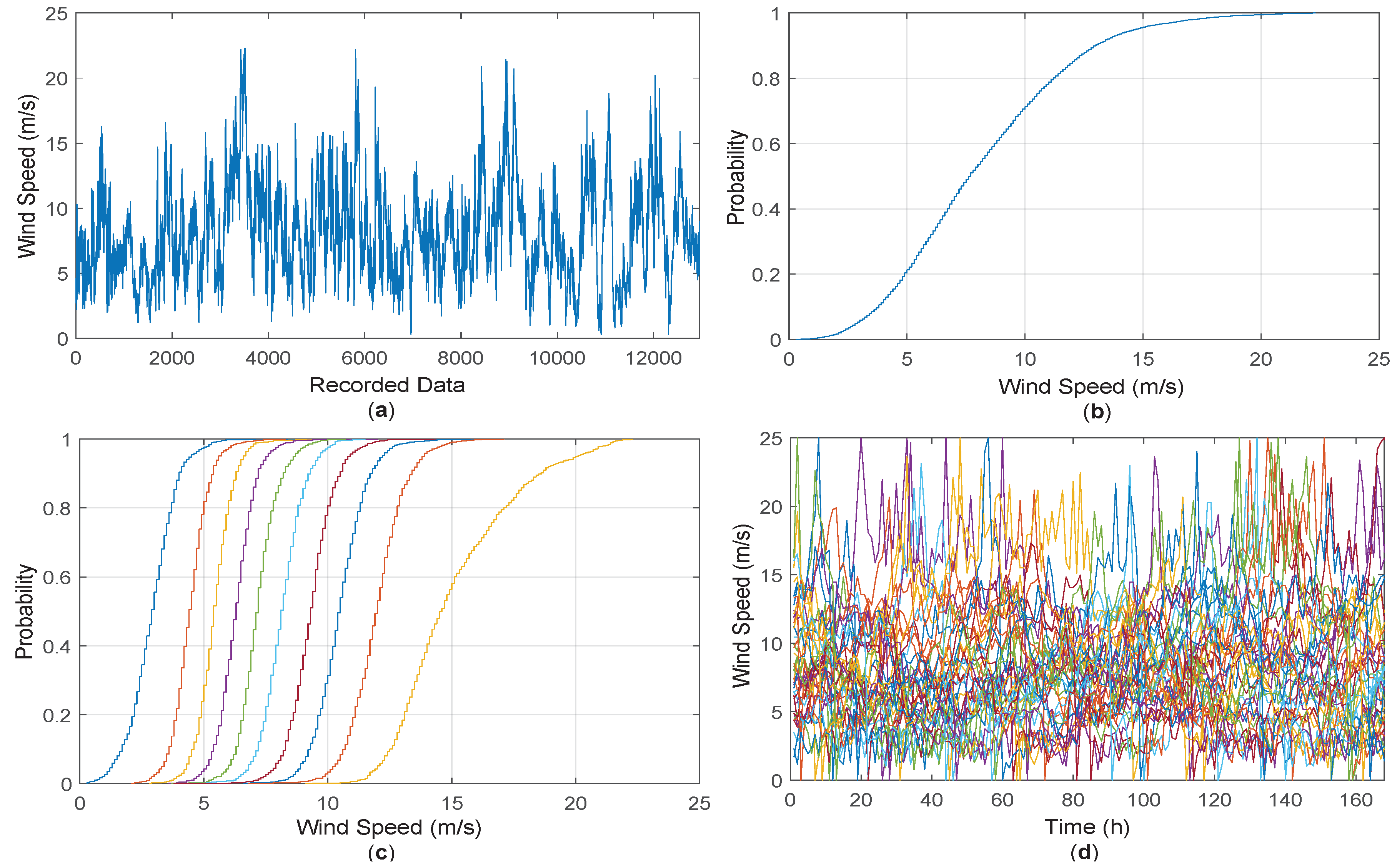
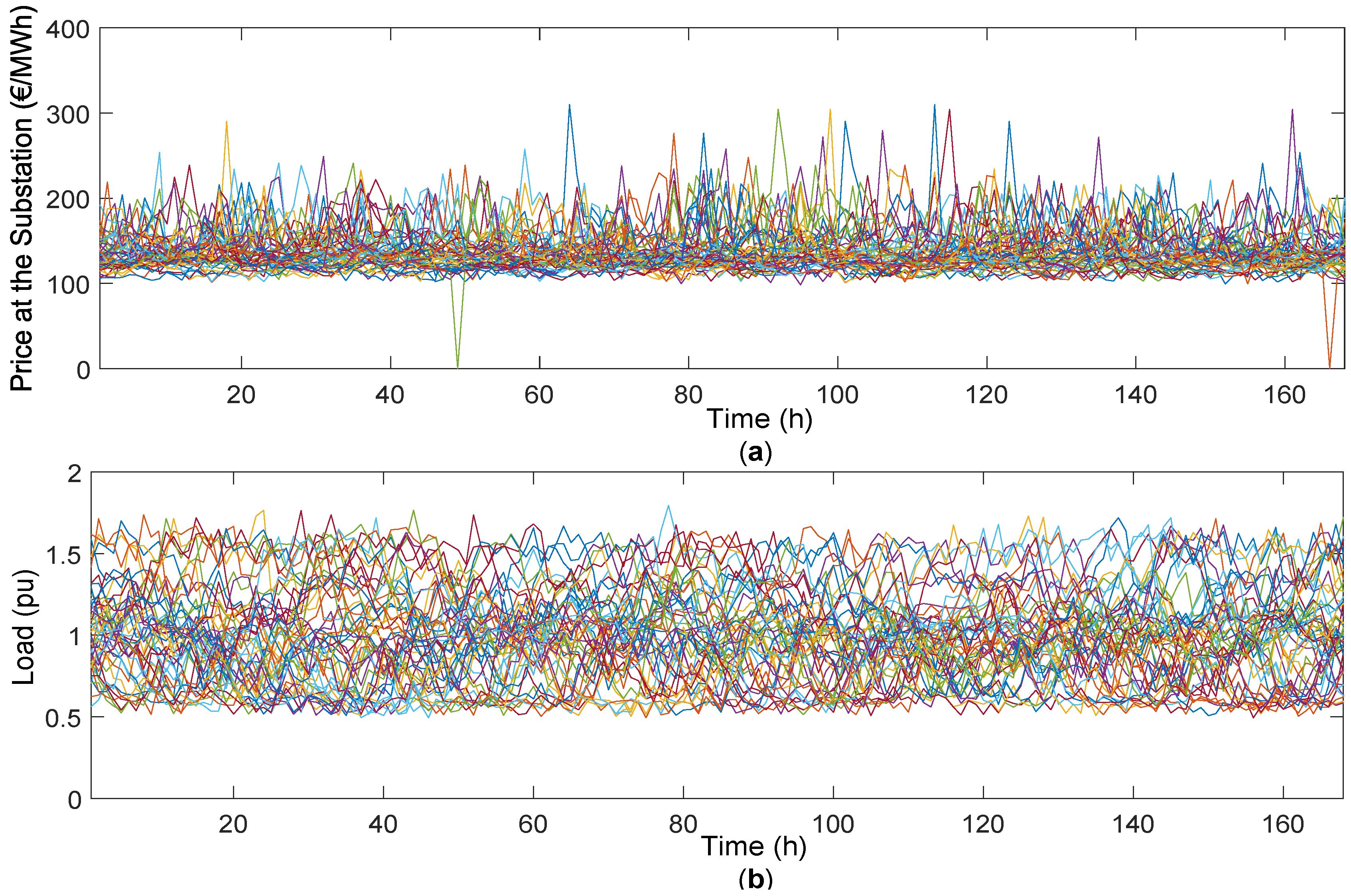
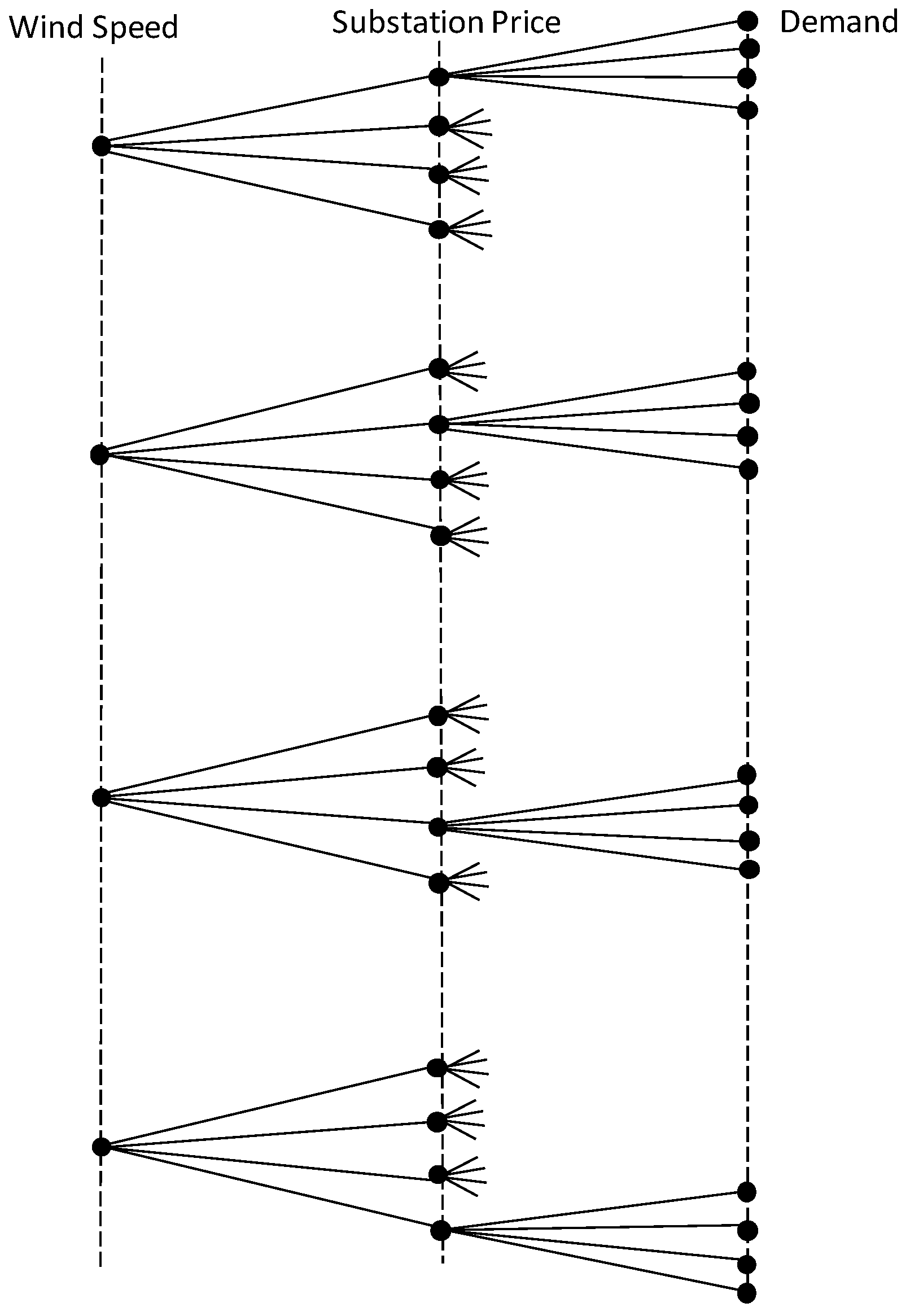
2.1. Scenario Generation

In the presence of renewable-based DG, it is necessary to consider the intermittency and uncertainty of these resources. Consequently, in order to model wind uncertainty, a probabilistic method based on time series has been implemented. Historical data of one year of wind speed is considered as initial data for candidate areas of wind generation. This section explains the generation of wind scenarios.

For each season, the cumulative distribution function (CDF) of historical wind speed is constructed. In Figure 1a, historical wind speed data for winter is represented. Initially, the number of scenarios is decided. Then, for each scenario, the initial value of wind speed is determined by a random number from a uniform probability distribution (0,1) that enters as the probability of the CDF of the historical data and identifies the corresponding wind value. The CDF of the historical data of winter is illustrated in Figure 1b. This methodology is known as the classical selection mechanism.

In order to select the next wind speed value, the CDF of the historical wind speed data has previously been divided into deciles, obtaining the wind speed ranges. For instance, in winter, wind speeds have the following limits: 3.85, 4.98, 5.92, 7, 7.95, 8.81, 9.93, 11.27, 13.08, 22.38 m/s. Taking all the wind speeds located in the same decile, the CDF corresponding to the wind speed of the historical data at the next step is constructed. The decile of the initial wind speed, for each scenario, is identified. The CDF of the wind speed at the next time step for that decile is considered, extracting the wind speed from that CDF with the classical selection mechanism indicated above. The decile of the wind speed extracted is identified, the corresponding CDF of the next time step is considered, the new wind speed is extracted, and this is performed successively until all the wind speed values in the time interval of analysis have been extracted. The CDF corresponding to the wind speed of the historical data at the next step for each decile is visualized in Figure 1c. Finally, wind scenarios are represented for one week in Figure 1d.

The same approach is done for substation prices and load scenarios as seen in Figure 2.

In order to have a tractable computational time, 50 scenarios have been generated for each input (wind, load, substation price) and they been reduced to four scenarios for each one of the inputs by using the k-means clustering algorithm. This method can be used to partition a given set of scenarios into a given number of clusters. As a result of this partition, scenarios with similar features are assigned to the same cluster. The centroid of each cluster represents a somewhat average pattern of all the scenarios included in a cluster. Since the centroid is artificial, the original scenario with the lowest probability distance from the centroid is used to represent the cluster. The relationship between the considered uncertainty sources is graphically described in Figure 3, resulting in 4³ scenarios. The number of scenarios has been limited to this figure to minimize the dimensionality in the problem formulation.

2.2. Generic Energy Storage Systems Modeling

Recently, the use of storage devices has increased significantly. In this work, an ideal and generic storage unit model is presented as in [26], which is “a device with the capability of transforming and storing energy, and reverting the process by injecting back the stored energy to the system”. Within this context, it can be conveniently integrated in complex optimization problems. An ideal and generic storage device is modeled with the hypothesis mentioned below:

• There are no up or down ramps.
• There are no storage energy losses.
• There is no hysteresis in discharging or charging.
• There are conversion losses. This means there are efficiency rates of direct (production) and reverse (storage) energy transformation. These rates are given with respect to the energy measured at the bus connected to the storage unit.
• Production/storage costs are the same for any level of production/storage of the unit.
• Energy production/storage occurs at constant power for the minimum period of study (typically one hour).
• The depth of discharge is assumed to be 80% of the maximum storage energy capacity.

The mathematical formulation of ESS is represented through Equations (1)–(5):

$$\begin{array}{c}{\underline{s}}_i^{\mathrm{s}}{\mathsf{\beta }}_i\le s_{it\mathsf{\omega }}^{\mathrm{s}}\le {\overline{s}}_i^{\mathrm{s}}{\mathsf{\beta }}_i\end{array}$$

(1)

$$\begin{array}{c}{\underline{s}}_i^{\mathrm{p}}{\mathsf{\beta }}_i\le s_{it\mathsf{\omega }}^{\mathrm{p}}\le {\overline{s}}_i^{\mathrm{p}}{\mathsf{\beta }}_i\end{array}$$

(2)

$$\begin{array}{c}{\underline{x}}_i\le x_{it\mathsf{\omega }}\le {\overline{x}}_i\end{array}$$

(3)

$$\begin{array}{c}{x}_{it\mathsf{\omega }}=x_{i(t-1)\mathsf{\omega }}+\Delta [{\mathsf{\eta }}_i^{\mathrm{s}}{s}_{it\mathsf{\omega }}^{\mathrm{s}}-(1/{\mathsf{\eta }}_i^{\mathrm{p}})s_{it\mathsf{\omega }}^{\mathrm{p}}]\end{array}$$

(4)

$$\begin{array}{c}{x}_{it=0\mathsf{\omega }}=x_{it=T\mathsf{\omega }}\end{array}$$

(5)

In the above equations, the actual storage (charge) and production (injection into the network) bounds are defined in Equations (1) and (2). A binary variable ${\mathsf{\beta }}_i$ for allocating EES in a node i of the network is introduced in these equations. Additionally, capacity limits of the ESS are introduced in Equation (3). Equation (4) shows the storage transition function. Thus, the state of charge, $x_{it\mathsf{\omega }}$ (storage level at bus i, period t and scenario $\mathsf{\omega }$), of the ESS located at bus i at the end of time interval t for each scenario $\mathsf{\omega }$ depends on the previous state of charge, $x_{i(t-1)\mathsf{\omega }}$, and the power storage/production during the current interval. In Equation (5), the initial energy status of the ESS has to be the same as that at the end of the period.

Finally, Equation (6) defines the location of ESS under different penetration levels (total number of EES units) in the model, ESS:

$$\sum _i{\mathsf{\beta }}_i=N^{\text{st}}$$

(6)

3. Mixed Integer Linear Programming Formulation

The following assumptions are made to represent a simplified power flow of a distribution system, generation and storage devices:

• The electric distribution system is a balanced three-phase system and can be represented by its equivalent single-phase circuit.
• The time stretch used for the simulation is one week, in intervals of time of 1 h.
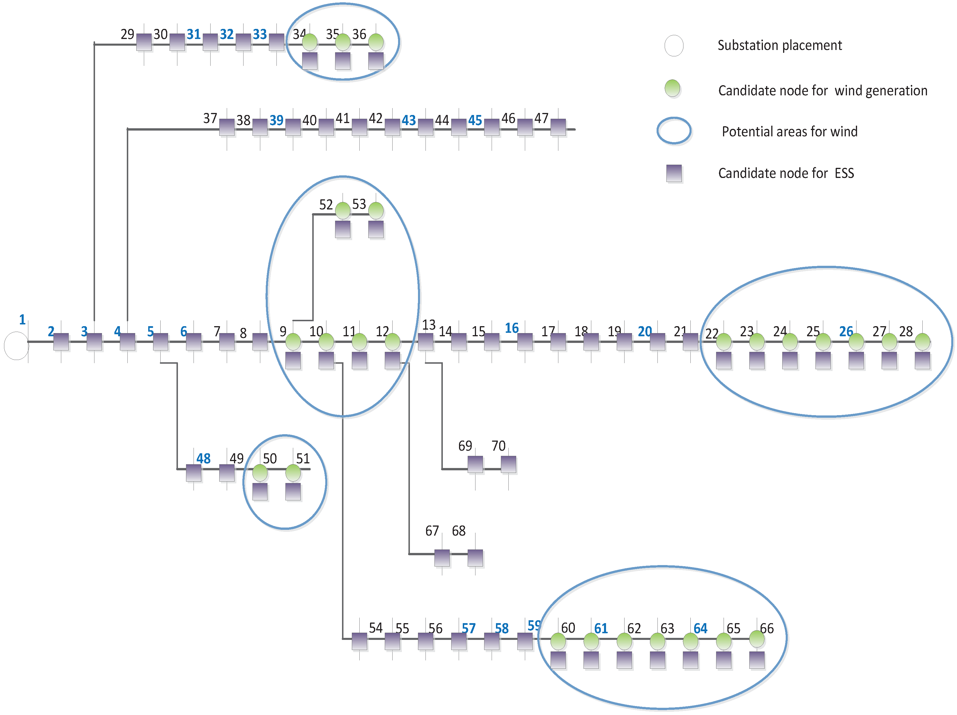
• Several candidate buses are selected for the optimal location of the wind unit. The optimal locations, based on wind resources, should be selected according to: high average speed, acceptable diurnal and seasonal variations, acceptable levels of turbulence and extreme winds. Other technical criteria are the softness of the orography for the civil works and the proximity of power lines with evacuation capacity for interconnection, technical feasibility and ease of construction or absence of environmental, urban, archaeological and cultural conditions.
• In the case of locating ESS, all the buses are candidates for location.
• For the sake of simplicity, only one wind power unit and one ESS unit are used. The variation of the installed amount of wind and ESS capacities at the optimal locations is discussed in the case study.

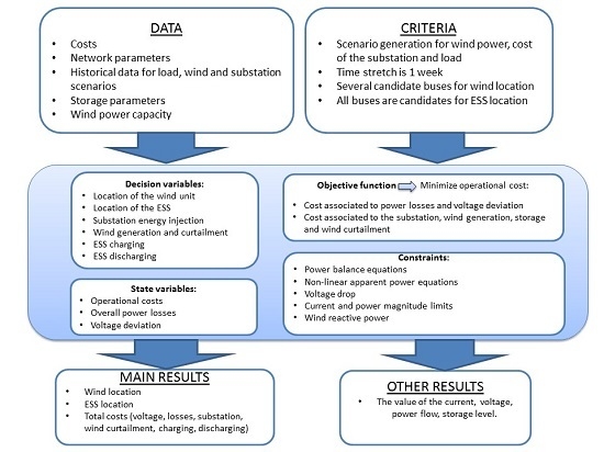
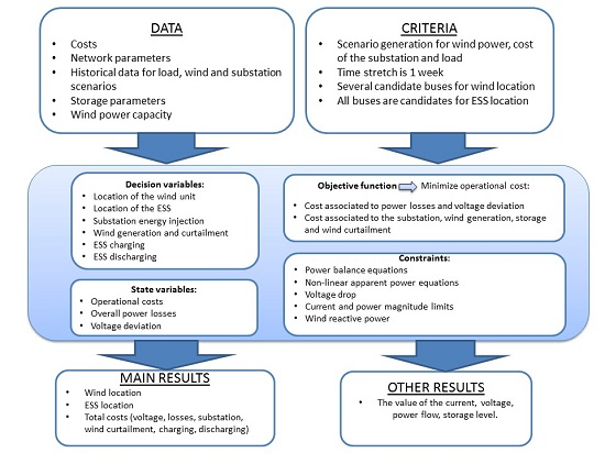
3.1. Objective Function

The aim of the optimization model proposed is to minimize all the costs associated with the operation of a distribution network and how the penetration of DG and ESS affects it. The objective function in Equation (7), the expected values of the total cost of the real power losses and the voltage deviation with respect to the reference value in branch i, j are penalized in Equation (8). The probability-weighted average of all possible values produces the expected values of the costs. Furthermore, the cost of the energy that comes from the substation, wind curtailment cost, and production and storage costs are also included in Equation (9):

$$\text{min}\left\{E\right[\mathsf{\psi }\left(\mathsf{\omega }\right)]+E[\mathsf{\kappa }\left(\mathsf{\omega }\right)\left]\right\}$$

(7)

$$\begin{array}{c}\hfill \mathsf{\psi }\left(\mathsf{\omega }\right)=\sum _t\sum _{ij}\Delta R_{ij}{I}_{ijt\mathsf{\omega }}^2{C}^{\text{loss}}+\sum _t\sum _{ij}\Delta \left|V_{it\mathsf{\omega }}^2-V_{\text{ref}}^2\right|C^{V_{\text{dev}}}/R_{\text{nom}}\end{array}$$

(8)

$$\begin{array}{c}\hfill \kappa \left(\mathsf{\omega }\right)=\sum _t\sum _i\Delta [P_{it\mathsf{\omega }}^{\text{sub}}{C}_{it\mathsf{\omega }}^{\text{sub}}+s_{it\mathsf{\omega }}^{\mathrm{p}}{C}^{\mathrm{p}}+s_{it\mathsf{\omega }}^{\mathrm{s}}{C}^{\mathrm{s}}+P_{it\mathsf{\omega }}^{\mathrm{w}\_\text{curt}}{C}^{\mathrm{w}\_\text{curt}}]\end{array}$$

(9)

3.2. Constraints

The objective function is subject to a set of constraints to assure optimal operational conditions.

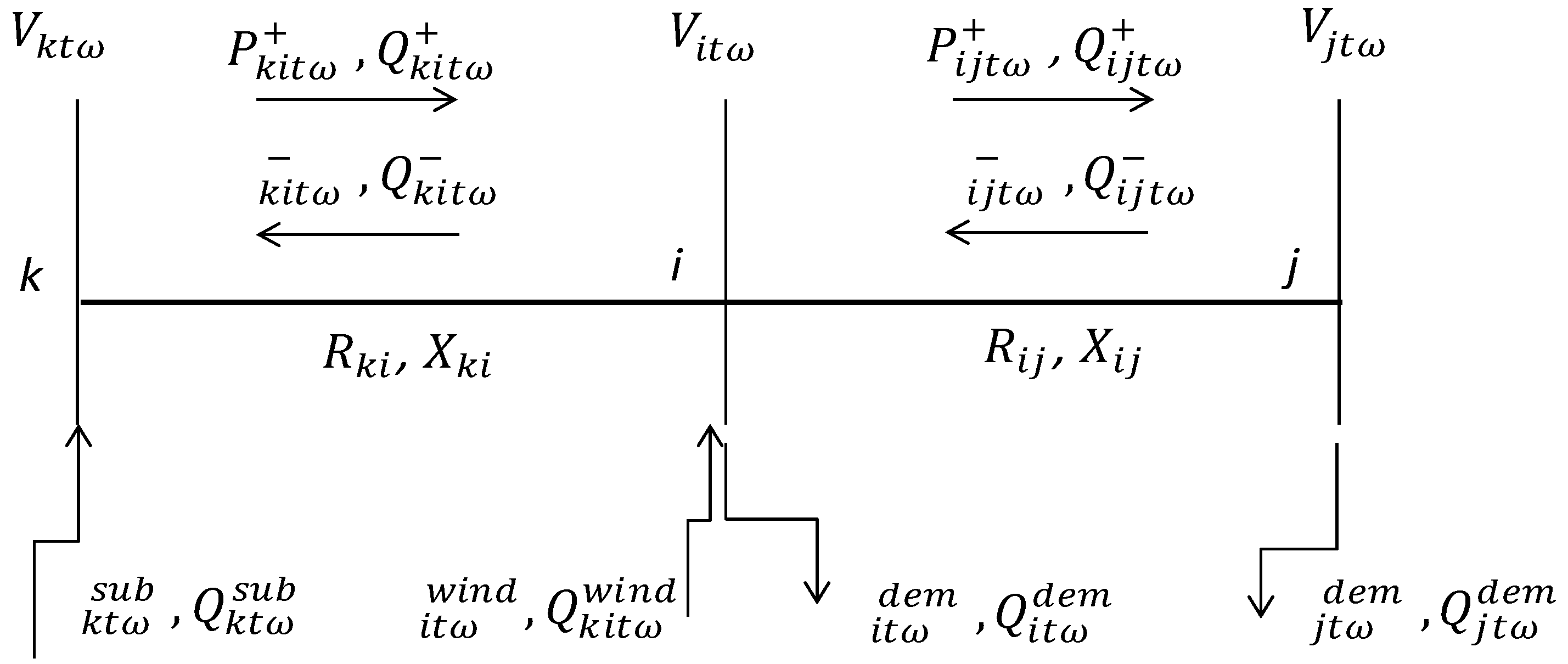
3.2.1. Power Balance Equations

Real wind power including curtailment is represented in Equation (10). This equation is active in the nodes where the model optimally locates the wind unit, and the active power injected comes from the wind power scenario generation discounting the wind power curtaiment, if necessary. The optimal location of wind power generation at bus i is defined by binary variable ${\mathsf{\alpha }}_i$:

$$\begin{array}{c}{P}_{it\mathsf{\omega }}^{\text{wind}}=P_{it\mathsf{\omega }}^{\mathrm{w}\_\text{fore}}{\mathsf{\alpha }}_i-P_{it\mathsf{\omega }}^{\mathrm{w}\_\text{curt}}\end{array}$$

(10)

$$\begin{array}{c}{\sum }_i{\mathsf{\alpha }}_i=N^{\text{wind}}\end{array}$$

(11)

Equation (11) defines the location of wind units under $N^{\text{wind}}$ different penetration levels of wind.

Real and reactive power balance equations at bus i are formulated in Equations (12) and (13). For both active and reactive power, wind power generation, production/storage of ESS, and the power flow from/to the substation are considered:

$$\begin{array}{c}{P}_{it\mathsf{\omega }}^{\text{sub}}+P_{it\mathsf{\omega }}^{\text{wind}}+{\sum }_{\mathrm{k}}(P_{\mathrm{k}it\mathsf{\omega }}^{+}-P_{\mathrm{k}it\mathsf{\omega }}^{-})-{\sum }_j[(P_{ijt\mathsf{\omega }}^{+}-P_{ijt\mathsf{\omega }}^{-})+R_{ij}{I}_{ijt\mathsf{\omega }}^2]+(s_{it\mathsf{\omega }}^{\mathrm{p}}-s_{it\mathsf{\omega }}^{\mathrm{s}})=P_{it\mathsf{\omega }}^{\text{dem}}\end{array}$$

(12)

$$\begin{array}{c}{Q}_{it\mathsf{\omega }}^{\text{sub}}+Q_{it\mathsf{\omega }}^{\text{wind}}+{\sum }_{\mathrm{k}}(Q_{\mathrm{k}it\mathsf{\omega }}^{+}-Q_{\mathrm{k}it\mathsf{\omega }}^{-})-{\sum }_j[(Q_{ijt\mathsf{\omega }}^{+}-Q_{ijt\mathsf{\omega }}^{-})+X_{ij}{I}_{ijt\mathsf{\omega }}^2]=Q_{it\mathsf{\omega }}^{\text{dem}}\end{array}$$

(13)

In order to distinguish the direction (sense) of the current and power flow (forward or downward the substation) due to existence of DG, especially in Equations (12) and (13), two types of positive separate variables are used for both active ($P_{ijt\mathsf{\omega }}^{+}$, $P_{ijt\mathsf{\omega }}^{-}$) and reactive power ($Q_{ijt\mathsf{\omega }}^{+}$, $Q_{ijt\mathsf{\omega }}^{-}$), as seen in Figure 4.

3.2.2. Non-Linear Apparent Power Equations

The current flow magnitude calculation is expressed by Equation (14), which is the only non-linear equation in the optimization model. The linearization procedure is explained in detail in Section 3.3:

$$\begin{array}{c}{V}_{jt\mathsf{\omega }}^2{I}_{ijt\mathsf{\omega }}^2=P_{ijt\mathsf{\omega }}^2+Q_{ijt\mathsf{\omega }}^2\end{array}$$

(14)

3.2.3. Voltage Drop Equations

Voltage drops between buses are formulated in Equation (15):

$$\begin{array}{c}\hfill V_{it\mathsf{\omega }}^2-Z_{ij}^2{I}_{ijt\mathsf{\omega }}^2-2[R_{ij}(P_{ijt\mathsf{\omega }}^{+}-P_{ijt\mathsf{\omega }}^{-})+X_{ij}(Q_{ijt\mathsf{\omega }}^{+}-Q_{ijt\mathsf{\omega }}^{-})]-V_{jt\mathsf{\omega }}^2=0\end{array}$$

(15)

The equation above is obtained from the initial phasor equation in Equation (16):

$$\begin{array}{c}\hfill \overrightarrow{V_i}-\overrightarrow{V_j}=\overrightarrow{I_{ij}}(R_{ij}+j{X}_{ij})\end{array}$$

(16)

The complex power expressed by the product that appears in Equation (17), where $\overrightarrow{V_i}$,$\overrightarrow{V_j}$,$\overrightarrow{I_{ij}}$ are voltages and currents, and $\overrightarrow{I_{ij}^{*}}$ is the complex conjugate of the current:

$$\begin{array}{c}\hfill \overrightarrow{V_j}\overrightarrow{I_{ij}^{*}}=P_{ij}+j{Q}_{ij}\end{array}$$

(17)

Substituting the current magnitude value of Equation (17) into Equation (16) leads to Equation (18):

$$\begin{array}{c}\hfill \overrightarrow{V_i}-\overrightarrow{V_j}=(P_{ij}+j{Q}_{ij}/\overrightarrow{V_j})*(R_{ij}+j{X}_{ij})\end{array}$$

(18)

By operating, this leads to Equation (19), where $\overrightarrow{V_i}$ is equal to its module $V_i$ and its phasor ${\mathsf{\theta }}_i$, and ${\mathsf{\theta }}_{ij}={\mathsf{\theta }}_i-{\mathsf{\theta }}_j$, obtaining Equation (20):

$$\begin{array}{c}(\overrightarrow{V_i}-\overrightarrow{V_j}){\overrightarrow{V_j}}^{*}=(P_{ij}-j{Q}_{ij})(R_{ij}+j{X}_{ij})\end{array}$$

(19)

$$\begin{array}{c}{V}_i{V}_j(\text{cos}\left({\mathsf{\theta }}_{ij}\right)+j\text{sin}\left({\mathsf{\theta }}_{ij}\right))=(P_{ij}-j{Q}_{ij})(R_{ij}+j{X}_{ij})\end{array}$$

(20)

Separating the real Equation (21) and imaginary parts Equation (22), we obtain:

$$\begin{array}{c}{V}_i{V}_j\text{cos}\left({\mathsf{\theta }}_{ij}\right)=P_{ij}{R}_{ij}+Q_{ij}{X}_{ij}+V_j^2\hfill \end{array}$$

(21)

$$\begin{array}{c}{V}_i{V}_j\text{sin}\left({\mathsf{\theta }}_{ij}\right)=P_{ij}{X}_{ij}-Q_{ij}{R}_{ij}\hfill \end{array}$$

(22)

Considering the relation $Z_{ij}^2=R_{ij}^2+X_{ij}^2$ and the trigonometric rule $\text{sin}{\mathsf{\theta }}_{ij}^2+\text{cos}{\mathsf{\theta }}_{ij}^2=1$, and summing the squares of Equations (21) and (22), we obtain the expression of the voltage drop:

$$\begin{array}{c}\hfill V_i^2-Z_{ij}^2{I}_{ij}^2-2[R_{ij}{P}_{ij}+X_{ij}{Q}_{ij}]-V_j^2=0\end{array}$$

(23)

Specifying Equation (23) in the model, with the inclusion of the direction of the power flow, this becomes Equation (15). Finally, the maximum and minimum voltage variations for bus i are defined in Equation (24):

$$\begin{array}{c}\hfill {\underline{V}}^2\le V_{it\mathsf{\omega }}^2\le {\overline{V}}^2\end{array}$$

(24)

3.2.4. Current and Power Magnitude Limits

Regarding thermal limits, a set of constraints is introduced for current in Equation (25), real power in Equations (26) and (27), and reactive power in Equations (28) and (29) limits, respectively. In addition, Equations (30) and (31) are set to avoid considering forward and backward power flows simultaneously. Note that Equations (26)–(29) are auxiliary constraints to improve the convergence of the proposed model:

$$\begin{array}{c}0\le I_{ijt\mathsf{\omega }}^2\le {\overline{I}}_{ij}^2\hfill \end{array}$$

(25)

$$\begin{array}{c}{P}_{jit\mathsf{\omega }}^{+}\le V_{\text{nom}}{\overline{I}}_{ij}{v}_{ijt\mathsf{\omega }}^{P^{+}}\hfill \end{array}$$

(26)

$$\begin{array}{c}{P}_{jit\mathsf{\omega }}^{-}\le V_{\text{nom}}{\overline{I}}_{ij}{v}_{ijt\mathsf{\omega }}^{P^{-}}\hfill \end{array}$$

(27)

$$\begin{array}{c}{Q}_{jit\mathsf{\omega }}^{+}\le V_{\text{nom}}{\overline{I}}_{ij}{v}_{ijt\mathsf{\omega }}^{Q^{+}}\hfill \end{array}$$

(28)

$$\begin{array}{c}{Q}_{jit\mathsf{\omega }}^{-}\le V_{\text{nom}}{\overline{I}}_{ij}{v}_{ijt\mathsf{\omega }}^{Q^{-}}\hfill \end{array}$$

(29)

$$\begin{array}{c}{v}_{ijt\mathsf{\omega }}^{P^{+}}+v_{ijt\mathsf{\omega }}^{P^{-}}\le 1\hfill \end{array}$$

(30)

$$\begin{array}{c}{v}_{ijt\mathsf{\omega }}^{Q^{+}}+v_{ijt\mathsf{\omega }}^{Q^{-}}\le 1\hfill \end{array}$$

(31)

3.2.5. Wind Reactive Power Equations

In order to coordinate real and reactive power, the limitations of reactive power for wind units are calculated in Equations (32)–(34):

$$\begin{array}{c}{Q}_{it\mathsf{\omega }}^{{\text{wind}}^{-}}=P_{it\mathsf{\omega }}^{\text{wind}}(tan(arccos(-P{F}_i^{\text{wind}})))\end{array}$$

(32)

$$\begin{array}{c}{Q}_{it\mathsf{\omega }}^{{\text{wind}}^{+}}=P_{it\mathsf{\omega }}^{\text{wind}}(tan(arccos\left(P{F}_i^{\text{wind}}\right)))\end{array}$$

(33)

$$\begin{array}{c}{Q}_{it\mathsf{\omega }}^{{\text{wind}}^{-}}\le Q_{it\mathsf{\omega }}^{\text{wind}}\le Q_{it\mathsf{\omega }}^{{\text{wind}}^{+}}\end{array}$$

(34)

3.3. Linearization Procedure

To create a linear equation from constraint Equation (14), the two sides of the equation should be managed separately. Note that $V_{it\mathsf{\omega }}^2$ and $I_{ijt\mathsf{\omega }}^2$ are variables that represent the square magnitude values of voltage and current, respectively, and they are used in Equations (12)–(25). The linearization process of Equation (14) is stated below.

• $V_{jt\mathsf{\omega }}^2{I}_{ijt\mathsf{\omega }}^2$: the left side of Equation (14) is handled by dividing $V_{jt\mathsf{\omega }}^2$ into small segments. Nevertheless, this leads to an increase in the number of binary variables and computation time. In distribution systems, voltage magnitudes are within a small range, so a constant value $V_{\text{ref}}^2$ can be approximated as the voltage magnitude for the first run of the model, in which binary variables are relaxed [27], as seen in Equation (35):

  $$\begin{array}{c}{V}_{jt\mathsf{\omega }}^2{I}_{ijt\mathsf{\omega }}^2\approx V_{\text{nom}}^2{I}_{ijt\mathsf{\omega }}^2\hfill \end{array}$$

  (35)

  Next, the model is run again and $V_{jt\mathsf{\omega }}^2$ takes the value resulting from the first run. Note that $V_{jt\mathsf{\omega }}^2$ hardly changes after the second run. Because of the limited range of voltage magnitude variation, this simplification has a small error.
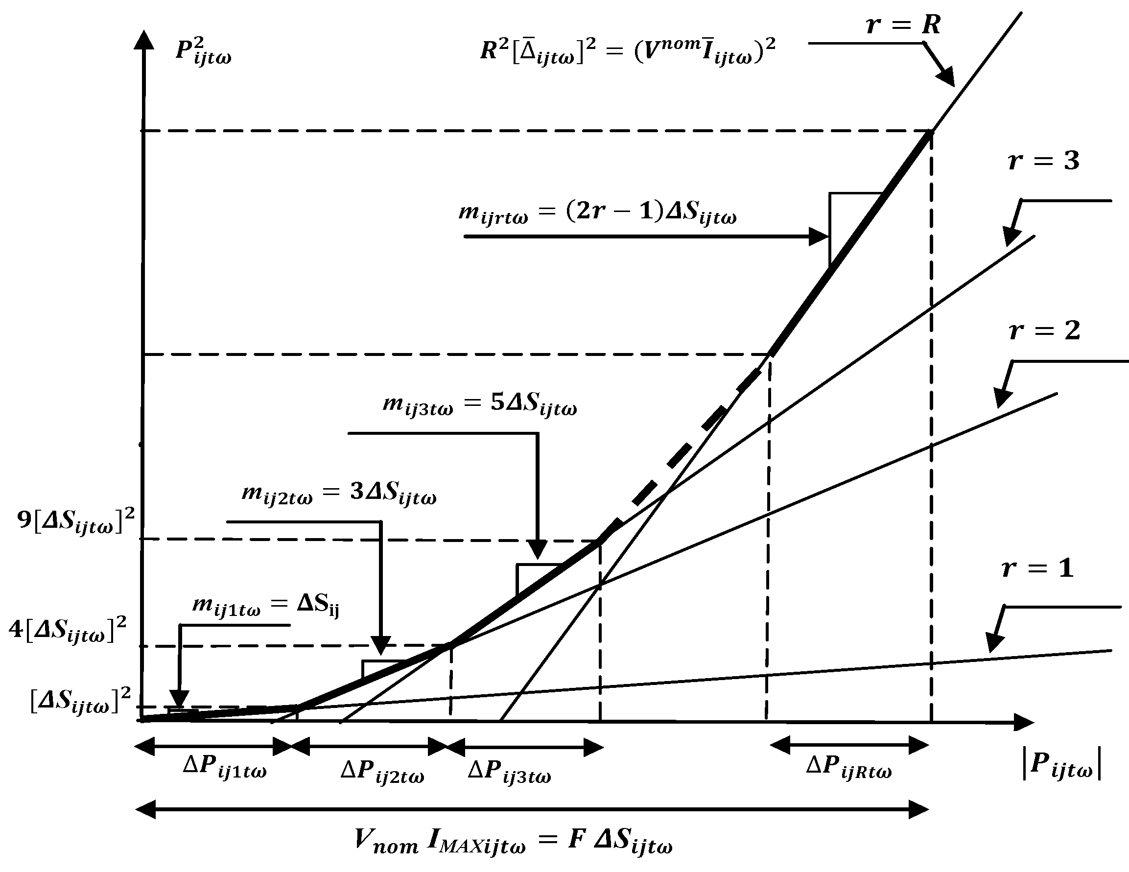
• $P_{ijt\mathsf{\omega }}^2+Q_{ijt\mathsf{\omega }}^2$: both terms on the right side of (Equation (14)) are handled by introducing a piecewise linear approximation [28]. The linearization process is the following:

  $$\begin{array}{c}{P}_{ijt\mathsf{\omega }}^2+Q_{ijt\mathsf{\omega }}^2={\sum }_r(m_{ijrt\mathsf{\omega }}\Delta P_{ijrt\mathsf{\omega }})\\ +{\sum }_r(m_{ijrt\mathsf{\omega }}\Delta Q_{ijt\mathsf{\omega }})\end{array}$$

  (36)

  $$\begin{array}{c}{P}_{ijt\mathsf{\omega }}^{+}+P_{ijt\mathsf{\omega }}^{-}={\sum }_r\Delta P_{ijrt\mathsf{\omega }}\end{array}$$

  (37)

  $$\begin{array}{c}{Q}_{ijt\mathsf{\omega }}^{+}+Q_{ijt\mathsf{\omega }}^{-}={\sum }_r\Delta Q_{ijrt\mathsf{\omega }}\end{array}$$

  (38)

  $$\begin{array}{c}0\le \Delta P_{ijrt\mathsf{\omega }}\le \Delta S_{ijrt\mathsf{\omega }}\end{array}$$

  (39)

  $$\begin{array}{c}0\le \Delta Q_{ijrt\mathsf{\omega }}\le \Delta S_{ijrt\mathsf{\omega }}\end{array}$$

  (40)

  where:

  $$\begin{array}{c}{m}_{ijrt\mathsf{\omega }}=(2r-1)\Delta S_{ijrt\mathsf{\omega }}\end{array}$$

  (41)

  $$\begin{array}{c}\Delta S_{ijrt\mathsf{\omega }}=\left(V_{\text{nom}}{\overline{I}}_{ij}\right)/R_{ij}\end{array}$$

  (42)

  Equation (36) is a piecewise linear approximation of ($P_{ijt\mathsf{\omega }}^2+Q_{ijt\mathsf{\omega }}^2$), and Equations (37) and (38) represent that ($P_{ijt\mathsf{\omega }}^{+}+P_{ijt\mathsf{\omega }}^{-}$) and ($Q_{ijt\mathsf{\omega }}^{+}+Q_{ijt\mathsf{\omega }}^{-}$) are equal to the sum of the values in each block of the discretization, which means they are a set of linear terms. In addition, $m_{ijrt\mathsf{\omega }}$ and ${\Delta S}_{ijrt\mathsf{\omega }}$ are constant parameters, and Equations (37) and (38) are linear expressions. Thus, Equation (43) represents the final linear form of constraint in Equation (14). In this equation, $V_{jt\mathsf{\omega }}^2$ is a parameter and ${\sum }_r(m_{ijrt\mathsf{\omega }}\Delta P_{ijrt\mathsf{\omega }})$ and ${\sum }_r(m_{ijrt\mathsf{\omega }}\Delta Q_{ijrt\mathsf{\omega }})$ are linear. The linearization of the active power Equation (14) is shown in Figure 5:

  $$\begin{array}{cc}\hfill V_{\text{ref}}^2{I}_{ijt\mathsf{\omega }}^2& ={\sum }_r\left(m_{ijrt\mathsf{\omega }}{\Delta P}_{ijrt\mathsf{\omega }}\right)+{\sum }_r\left(m_{ijrt\mathsf{\omega }}{\Delta Q}_{ijrt\mathsf{\omega }}\right)\end{array}$$

  (43)

4. Case Studies

4.1. Network Overview

The network used for the optimal location of both wind generation and ESS is the IEEE 69-bus system shown in Figure 6, where the bus numbers in blue are buses that are not connected to loads (as in [29]) and the candidate buses for both wind and ESS are represented. The maximum current flow through the branches is 150 A and network parameters are given in [29]. Since the voltage values vary through iterations, the voltage range is between 1.1 pu and 0.9 pu. In the linearization, 20 discrete blocks are considered since the solutions hardly change from 20 blocks onwards in the piecewise linearization procedure.

In order to generate scenarios, explained in Section 2.1, historical data of one year of wind speed is considered as initial data [30] and historical load values and generation prices are collected every hour from the Iberian Electricity Market for the extrapeninsular electric system Majorca-Menorca [31] for one year. The costs of power losses, voltage deviation and wind curtailment, production of the storage (discharging) and storage (charging) cost are $15/MWh, $15/MWh and $500/MWh.

The base power is 1 MVA and the installed power for wind generation can be either 1000 kW or 1500 kW for the different cases. The generic energy storage unit [32] can have different energy capacities: 500 kWh, 1000 kWh, and 1500 kWh, where the maximum storage/production power ranges between 100 kW and 1200 kW. The minimum storage/production power is set to 0. The initial energy level is set to 50% of its capacity. The efficiency rates to store or produce are set to 85%. The costs of production of the storage (discharging) and storage (charging) $0.1/MWh and $0.5/MWh, as in [25,26,28].

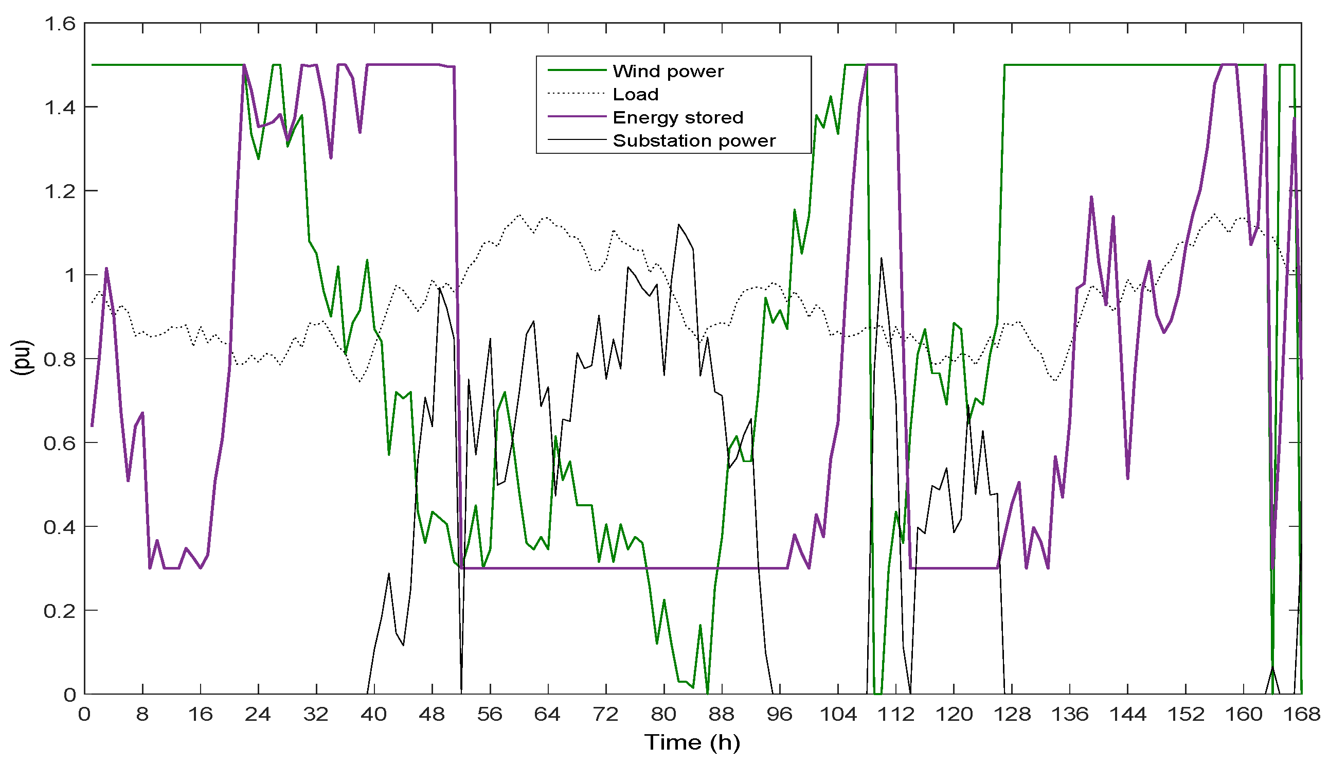
4.2. Simulation Results

This section shows the optimal location buses and describes the results of the operating costs: losses of the distribution network, substation, energy storage/production, wind curtailment and the voltage for selected cases studies. Different installed power/capacity levels of one wind unit and 1 EES unit are analyzed in the following independent cases, including a case without any unit (Case 1) and another with only high penetration of wind (Case 10), as seen in

Table 2. Characterization of the different case studies.

Values (pu)	Case 1	Case 2	Case 3	Case 4	Case 5	Case 6	Case 7	Case 8	Case 9	Case 10
Wind Power	0	1	1	1	1	1.5	1.5	1.5	1.5	1.5
ESS Capacity	0	0.5	0.5	1	1	1	1	1.5	1.5	0
ESS Max Power	0	0.1	0.4	0.2	0.8	0.2	0.8	0.3	1.2	0

.

The optimal locations, in which binary variables (${\mathsf{\alpha }}_i$ and ${\mathsf{\beta }}_i$) are active, are obtained for the different case studies as seen in

Table 3. Optimal location of wind generation and storage generation.

Cases	Case 1	Case 2	Case 3	Case 4	Case 5	Case 6	Case 7	Case 8	Case 9	Case 10
Wind Location	-	62	62	62	62	62	62	62	62	62
ESS Location	-	62	62	62	62	9	9	62	62	-

.

It can be seen that, in all the cases studies, the location of wind generation is at bus 62, which has the highest demand of the system. Thus, basically, the wind power production feeds that bus and the excess is provided to the network to feed the loads nearby or being stored in the ESS. Mainly, the storage device is co-located at the same bus, except for the cases in which the storage value is 1 pu and wind power is 1.5 pu, resulting in its placement at bus 9.

As seen in

Table 4. The model solution for all the cases.

Costs ($)	Case 1	Case 2	Case 3	Case 4	Case 5
Total	27,170	14,294	14,236	14,193	14,118
Voltage	120	70	71	70	72
Losses	147	110	102	102	95
Substation	26,902	14,114	14,063	14,021	13,951
Wind curtailment	-	-	-	-	-
Discharging	-	0.85	1.89	1.49	2.64
Charging	-	1.04	2.34	1.84	3.26
Costs ($)	Case 6	Case 7	Case 8	Case 9	Case 10
Total	10,395	10,250	10,121	10,025	15,471
Voltage	59	64	70	69	148
Losses	140	137	112	107	296
Substation	10,196	10,049	9,940	9,849	10,493
Wind curtailment	-	-	-	-	4,534
Discharging	5.34	15.60	5.98	20.68	-
Charging	6.60	19.26	7.38	25.53	-

, increasing the capacity of wind generation significantly decreases the production cost of the network for one week. Network losses are also reduced if the installed wind capacity is 1 pu. However, considering a high installed capacity of wind, real power losses are increased, as seen in Cases 6–10.

It is also desirable to have an ESS unit with a high value of maximum production/storage power because the device is less constrained to charge or discharge when it is required by the network. In this case, the cost of the energy that comes from the substation slightly decreases as seen between Cases 2 and 3. It is clear that increasing the installed capacity of storage can benefit the operational cost as it has more capacity to charge or discharge depending on the production cost in that hour (see the difference between Cases 6 and 8, and also Cases 7 and 9). In addition, network losses are decreased when the storage capacity increases from 1 pu to 1.5 pu while voltage deviation is slightly worse.

The behavior of storage depends on whether it is charging or discharging. Storage absorbs the excess of wind in periods when it exceeds the total load of the system. In other situations in which there is high wind and high load, ESS can also absorb energy in order not to violate the technical constraints of the distribution network. The ESS injects energy in the network when the production cost of the whole system is more expensive. Furthermore, another advantage of ESS is that they avoid wind power curtailment and its corresponding cost as it happens in Case 10. In this case, there are some hours in which wind generation is higher than load, which means that this power cannot be evacuated as the substation can only import power upstream; however, it cannot export power upstream. In the new context of increasing renewable energy in networks, ESS is a key element to deal with these situations and avoid wind curtailment. In addition, the effect of increasing the maximum power of the ESS for the same energy capacity, as seen in Case 7 with respect to Case 6, is that the ESS charges and discharges much more than in Case 6. This also reduces the injection from the substation and the overall costs making it a more flexible system that can react to the stochasticity of wind production.

Figure 7 shows the behavior of storage for some of the scenarios. The initial and final levels of energy in the ESS are equal to 0.75. It is observed that, depending on the value of wind power and demand in the distribution system at a certain hour, the behavior of storage is different. At the beginning of the time horizon, wind power is at its maximum level, so the ESS is charged up to hour 22, except for the hours when demand slightly increases (hour 4), in which the ESS discharges a bit without the need for the substation to supply. After hour 22, wind generation decreases, thus the ESS produces during the hours when the drop in wind production is more pronounced. At hour 52, the ESS discharges until its minimum value is reached, 0.3 pu, as we assumed a depth of discharge of 80% of the maximum ESS capacity (1.5 pu in this case), remaining at this value later on. This is a consequence of having low wind and a demand increase. In this situation, the substation begins to inject power into the network, as wind remains low. After that, wind production increases again (hour 96) and the ESS stores energy, meanwhile the substation decreases its injection until reaching 0 again. To sum up, under high wind, the ESS charges sharply if the demand is low and slightly if the demand is medium. It injects power at low wind levels and high demand.

5. Conclusions

A new model for the joint allocation of wind power generation and generic ESS has been implemented in this paper. In order to optimize the operation of a distribution system, a model is proposed to select the best allocation of wind and ESS within a linear AC OPF representing the performance of the model. To demonstrate the capability of the proposed stochastic procedure, it has been applied to an IEEE 69-bus system, where load, price at the substation, and wind scenarios are also considered. It can be concluded that: (i) the proposed MILP is well suited for finding the proper locations of wind and ESS; (ii) total operating costs are reduced with the combination of these technologies; (iii) the benefit of integrating ESS in a distributed network with wind power units is demonstrated.

References

1. Ackermann, T.; Andersson, G.; Söder, L. Distributed generation: A definition. Electr. Power Syst. Res. 2001, 57, 195–204. [Google Scholar] [CrossRef]
2. Liu, Z.; Wen, F.; Ledwich, G. Optimal siting and sizing of distributed generators in distribution systems considering uncertainties. IEEE Trans. Power Deliv. 2011, 26, 2541–2551. [Google Scholar] [CrossRef]
3. Korpaas, M.; Holen, A.T.; Hildrum, R. Operation and sizing of energy storage for wind power plants in a market system. Int. J. Electr. Power Energy Syst. 2003, 25, 599–606. [Google Scholar] [CrossRef]
4. Halamay, D.A.; Brekken, T.K.A.; Simmons, A.; McArthur, S. Reserve requirement impacts of large-scale integration of wind, solar, and ocean wave power generation. IEEE Trans. Sustain. Energy 2011, 2, 321–328. [Google Scholar] [CrossRef]
5. Vázquez, M.A.O.; Kirschen, D.S. Estimating the spinning reserve requirements in systems with significant wind power generation penetration. IEEE Trans. Power Syst. 2009, 24, 114–124. [Google Scholar] [CrossRef]
6. Srivastava, A.K.; Kumar, A.A.; Schulz, N.N. Impact of distributed generations with energy storage devices on the electric grid. IEEE Syst. J. 2012, 6, 110–117. [Google Scholar] [CrossRef]
7. Barton, J.; Infield, D. Energy storage and its use with intermittent renewable energy. IEEE Trans. Energy Convers. 2004, 19, 441–448. [Google Scholar] [CrossRef]
8. Schainker, R. Executive overview: Energy storage options for a sustainable energy future. In Proceedings of the IEEE Power Engineering Society General Meeting, Denver, CO, USA, 10 June 2004.
9. Leonhard, W.; Grobe, E. Sustainable electrical energy supply with wind and pumped storage—A realistic long-term strategy or Utopia? In Proceedings of the IEEE Power Engineering Society General Meeting, Denver, CO, USA, 10 June 2004.
10. Georgilakis, P.S.; Hatziargyriou, N.D. Optimal distributed generation placement in power distribution networks: Models, methods, and future research. IEEE Trans. Power Syst. 2013, 28, 3420–3428. [Google Scholar] [CrossRef]
11. Kumar, A.; Gao, W. Optimal distributed generation location using mixed integer non-linear programming in hybrid electricity markets. IET Gener. Transm. Distrib. 2010, 4, 281–298. [Google Scholar] [CrossRef]
12. Gandomkar, M.; Vakilian, M.; Ehsan, A. Genetic-based tabu search algorithm for optimal DG allocation in distribution networks. Electr. Power Compon. Syst. 2005, 12, 1351–1362. [Google Scholar] [CrossRef]
13. Ochoa, L.F.; Harrison, G.P. Minimizing energy losses: Optimal accommodation and smart operation of renewable distributed generation. IEEE Trans. Power Syst. 2011, 26, 198–205. [Google Scholar] [CrossRef]
14. Hung, D.Q.; Mithulananthan, N. Multiple distributed generator placement in primary distribution networks for loss reduction. IEEE Trans. Ind. Electron. 2013, 60, 1700–1708. [Google Scholar] [CrossRef]
15. Al Abri, R.S.; El-Saadany, E.F.; Atwa, Y.M. Optimal placement and sizing method to improve the voltage stability margin in a distribution system using distributed generation. IEEE Trans. Power Syst. 2013, 28, 326–334. [Google Scholar] [CrossRef]
16. Othman, M.M.; El-Khattam, W.; Hegazy, Y.G.; Abdelaziz, A.Y. Optimal placement and sizing of distributed generators in unbalanced distribution systems using supervised Big Bang-Big Crunch method. IEEE Trans. Power Syst. 2015, 30, 911–919. [Google Scholar] [CrossRef]
17. Karanki, S.B.; Xu, D.; Venkatesh, B.; Singh, B.N. Optimal location of battery energy storage systems in power distribution network for integrating renewable energy sources. In Proceeings of the IEEE Energy Conversion Congress and Exposition (ECCE), Denver, CO, USA, 15–19 September 2013.
18. Atwa, Y.M.; El-Saadany, E.F. Optimal allocation of ESS in distribution systems with a high penetration of wind energy. IEEE Trans. Power Syst. 2010, 25, 1815–1822. [Google Scholar] [CrossRef]
19. Akhavan-Hejazi, H.; Mohsenian-Rad, H. Optimal operation of independent storage systems in energy and reserve markets with high wind penetration. IEEE Trans. Smart Grid 2014, 5, 1088–1097. [Google Scholar] [CrossRef]
20. Alnaser, S.W.; Ochoa, L.F. Optimal sizing and control of energy storage in wind power-rich distribution networks. IEEE Trans. Power Syst. 2015, 31, 2004–2013. [Google Scholar] [CrossRef]
21. Ghofrani, M.; Arabali, A. A stochastic framework for power system operation with wind generation and energy storage integration. In Proceedings of the Innovative Smart Grid Technologies Conference (ISGT), Washington, DC, USA, 19–22 February 2014.
22. Xu, Y.; Jewell, W.T.; Pang, C. Optimal location of electrical energy storage unit in a power system with wind energy. In Proceedings of the North American Power Symposium (NAPS), Pullman, WA, USA, 7–9 September 2014.
23. Zhao, H.; Wu, Q.; Huang, S.; Guo, Q.; Sun, H.; Xue, Y. Optimal siting and sizing of energy storage System for power systems with large-scale wind power integration. In Proceedings of the Eindhoven PowerTech, Eindhoven, The Netherlands, 29 June–2 July 2015.
24. Nick, M.; Hohmann, M.; Cherkaoui, R.; Paolone, M. Optimal location and sizing of distributed storage systems in active distribution networks. In Proceedings of the IEEE 2013 PowerTech, Grenoble, France, 16–20 June 2013.
25. Meneses de Quevedo, P.; Allahdadian, J.; Contreras, J.; Chicco, G. Islanding in distribution systems considering wind power and storage. Sustain. Energy Grids Netw. 2016, 5, 156–166. [Google Scholar] [CrossRef]
26. Pozo, D.; Contreras, J.; Sauma, E.E. Unit commitment with ideal and generic energy storage units. IEEE Trans. Power Syst. 2014, 29, 2974–2984. [Google Scholar] [CrossRef]
27. Tabares Pozos, A.; Lavorato de Oliveira, M.; Franco Baquero, J.F.; Rider Flores, M.J. A mixed-binary linear formulation for the distribution system expansion planning problem. In Proceedings of the IEEE Transmission & Distribution Conference and Exposition—Latin America (PES T&D-LA), Medellin, Colombia, 10–13 September 2014; pp. 156–166.
28. Meneses de Quevedo, P.; Contreras, J.; Rider, M.J.; Allahdadian, J. Contingency assessment and network reconfiguration in distribution grids including wind power and energy storage. IEEE Trans. Sustain. Energy 2015, 6, 1524–1533. [Google Scholar] [CrossRef]
29. Chiang, H.; Jean-Jumeau, R. Optimal network reconfigurations in distribution systems. II. Solution algorithms and numerical results. IEEE Trans. Power Deliv. 1990, 5, 1568–1574. [Google Scholar] [CrossRef]
30. Meteorología y climatología de Navarra. 2014. Available online: http://meteo.navarra.es/estaciones/mapadeestaciones.cfm (assessed on 8 July 2016).
31. Red Eléctrica de España. SEIE: Demand and Generation Price. 2014. Available online: https://www.esios.ree.es/es (assessed on 8 July 2016).
32. AECOM, Australian Renewable Energy Agency. 2015. Available online: http://arena.gov.au/files/2015/07/AECOM-Energy-Storage-Study.pdf/ (assessed on 8 July 2016).
Figure 1. Method for wind scenario generation: (a) wind speed data for winter season; (b) cumulative distribution curve for winter season; (c) cumulative distribution curve for the 10 deciles; and (d) wind scenarios.
Energies 09 00528 g001
Figure 2. Substation price and load scenarios: (a) price at the substation (/MWh); and (b) load (pu).
Energies 09 00528 g002
Figure 3. Considered scenario tree for wind power generation, substation price and load.
Energies 09 00528 g003
Figure 4. Illustrative radial network with DG.
Energies 09 00528 g004
Figure 5. Modeling piecewise linear function P i j t ω 2 .
Energies 09 00528 g005
Figure 6. 69-bus network topology.
Energies 09 00528 g006
Figure 7. Energy stored in Case 9 in one scenario.
Energies 09 00528 g007