
Investigation of a Novel Mechanical to Thermal Energy Converter Based on the Inverse Problem of Electric Machines


Abstract
:1. Introduction
2. Thermal Power Analysis
2.1. Thermal Power Calculation
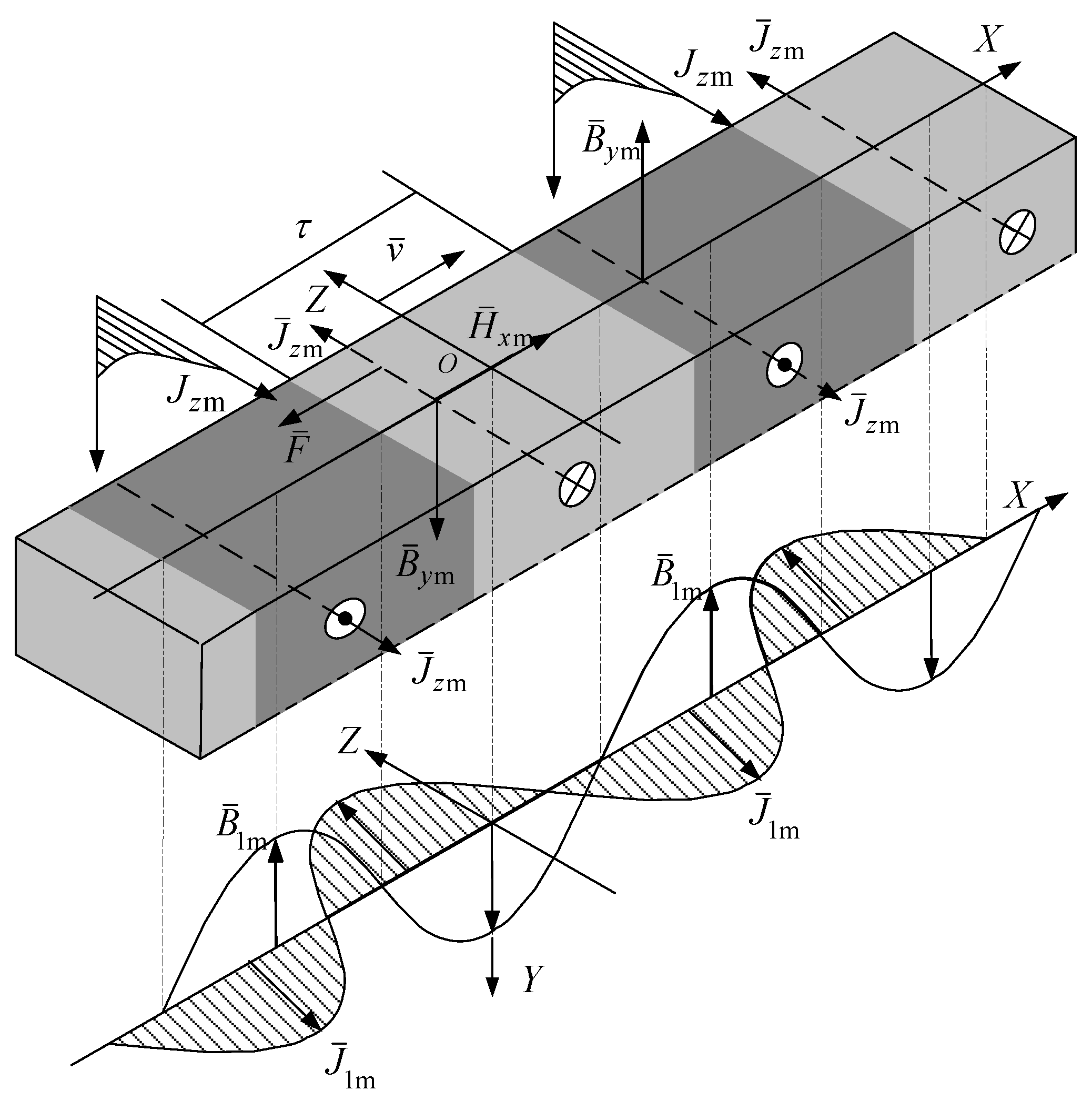
2.1.1. Eddy Current Thermal Power
2.1.2. Hysteresis Thermal Power
2.1.3. Calculation Result
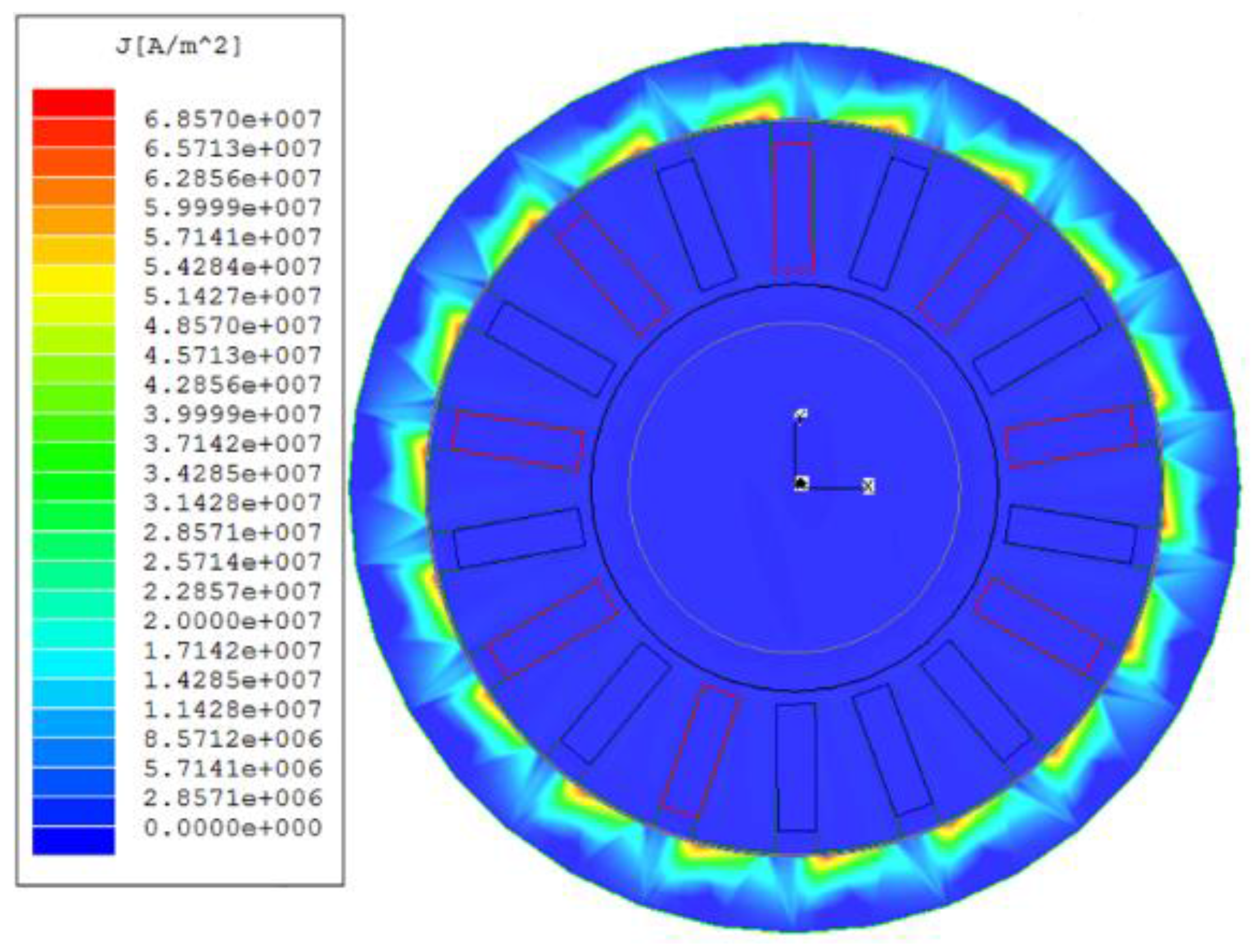
2.2. Eddy Current Distribution
3. Temperature Calculation
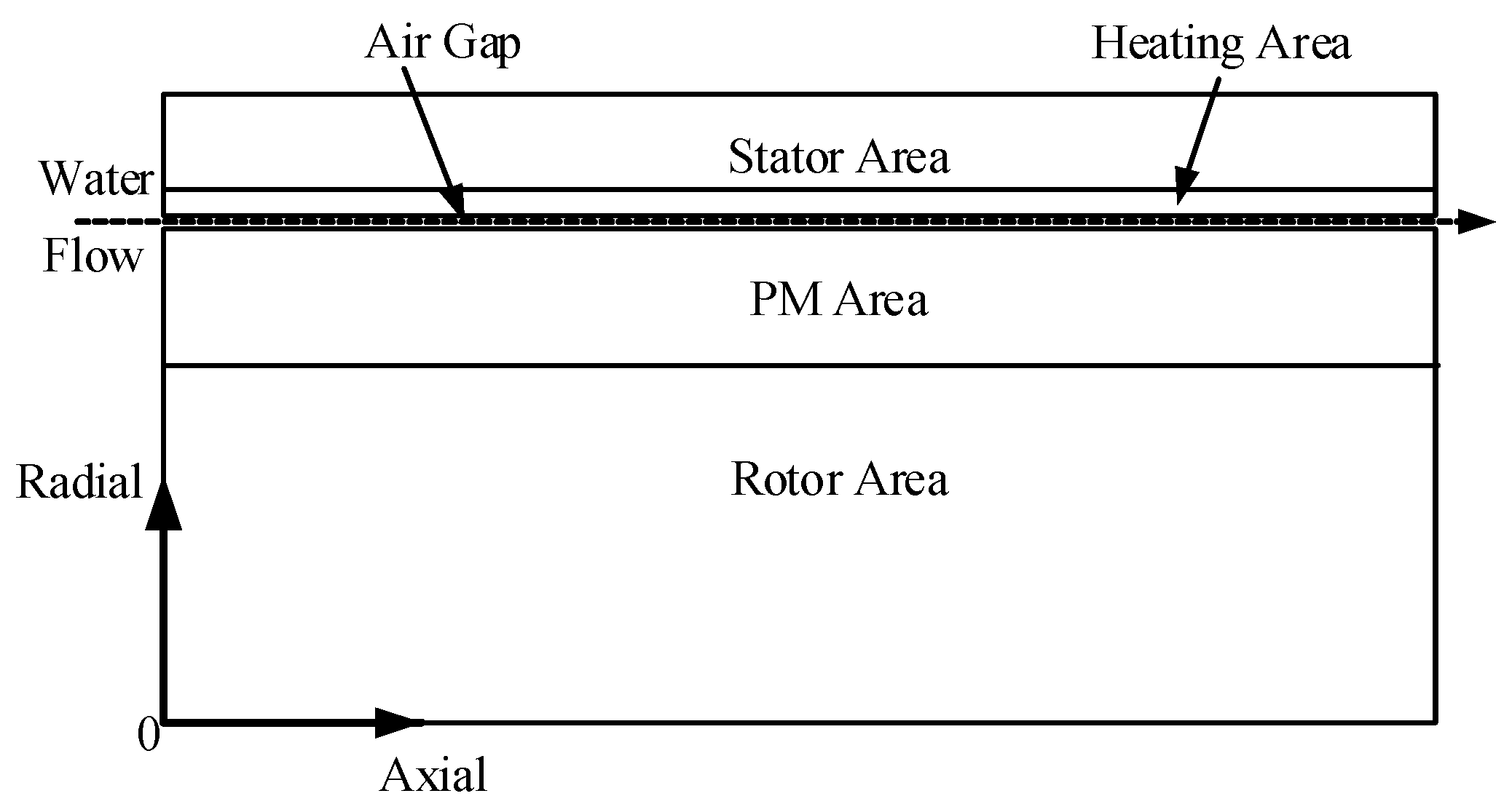
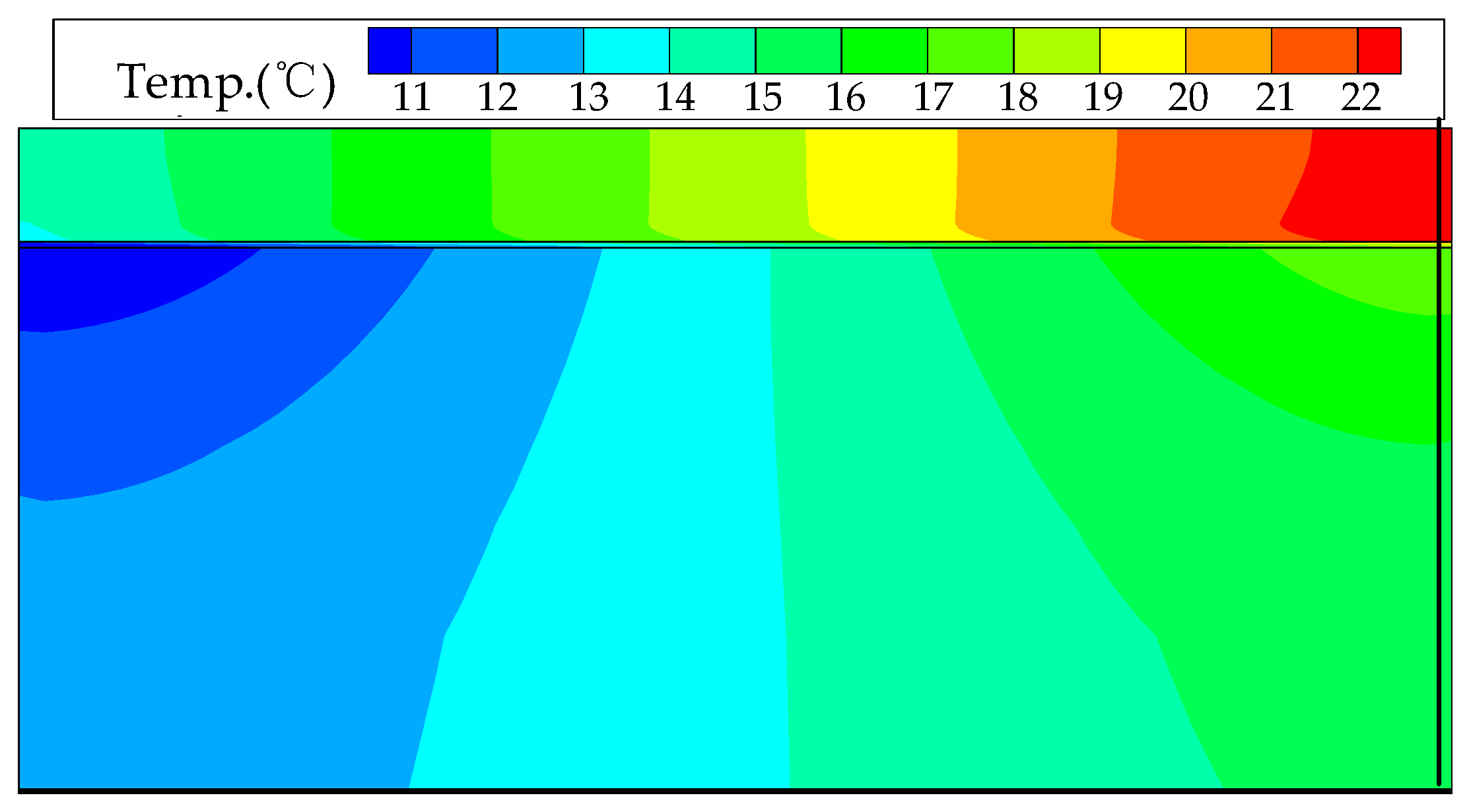
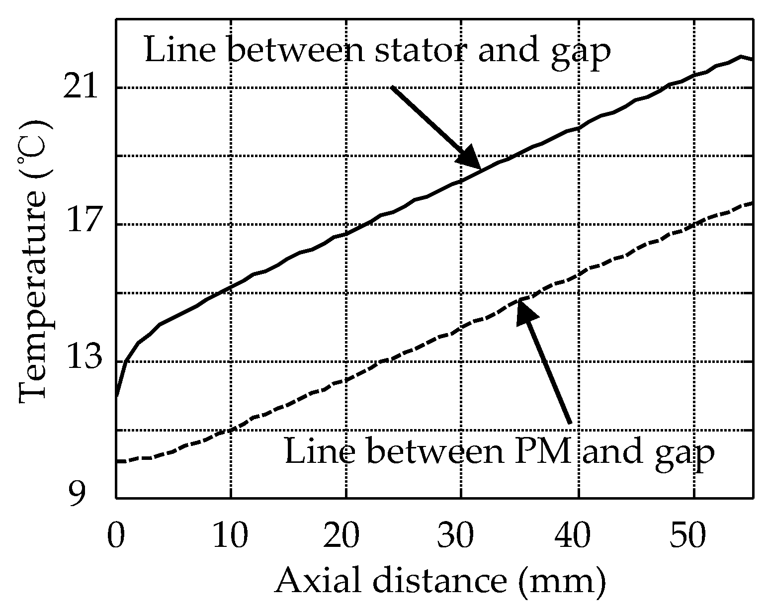
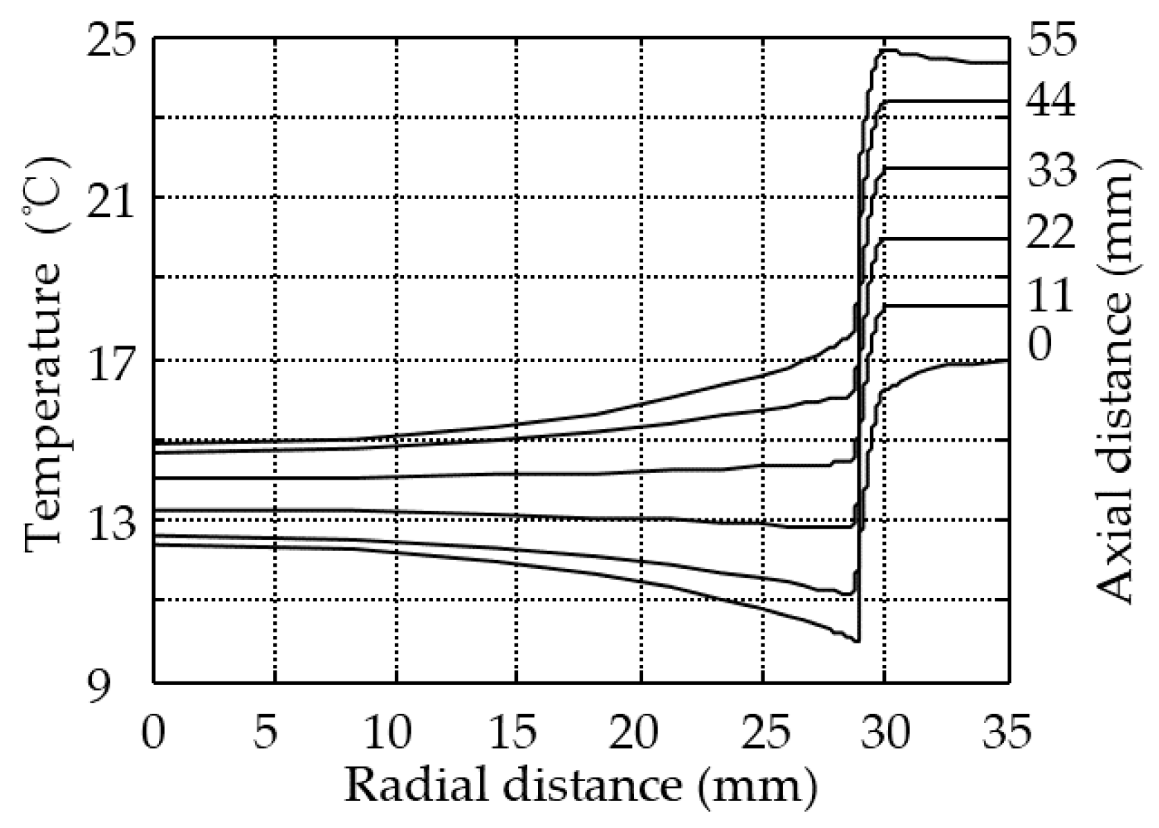
3.1. Temperature Field Calculation
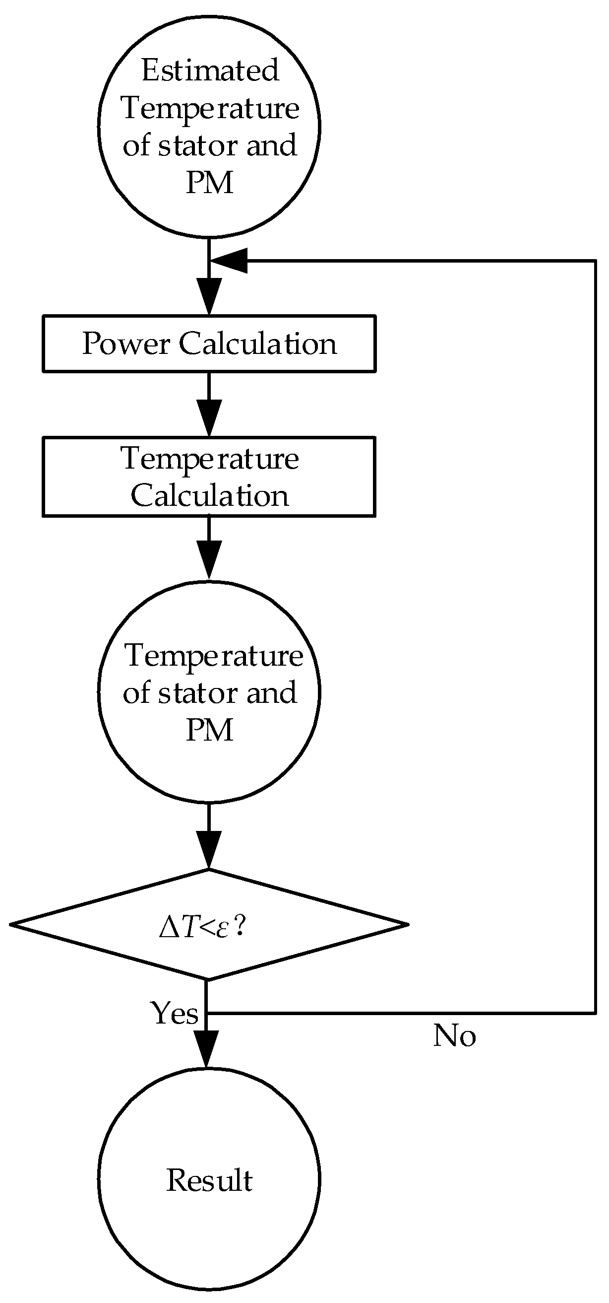
3.2. Thermal Power–Temperature Coupled Calculation Method
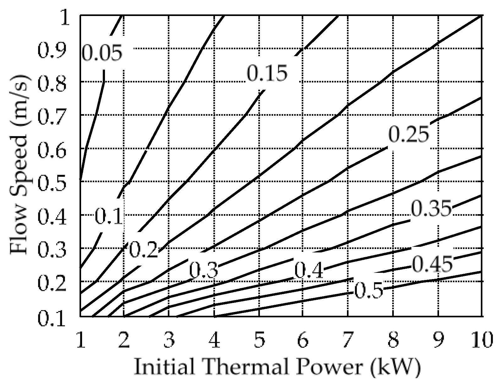
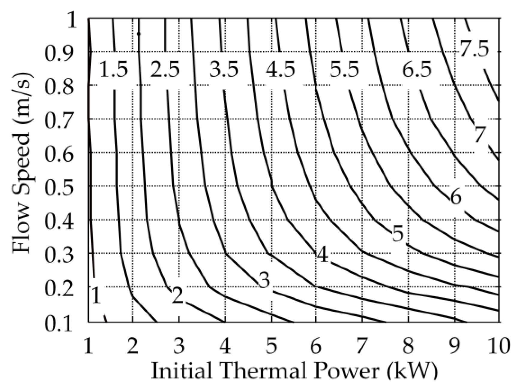
4. Operating Characteristic of the Converter
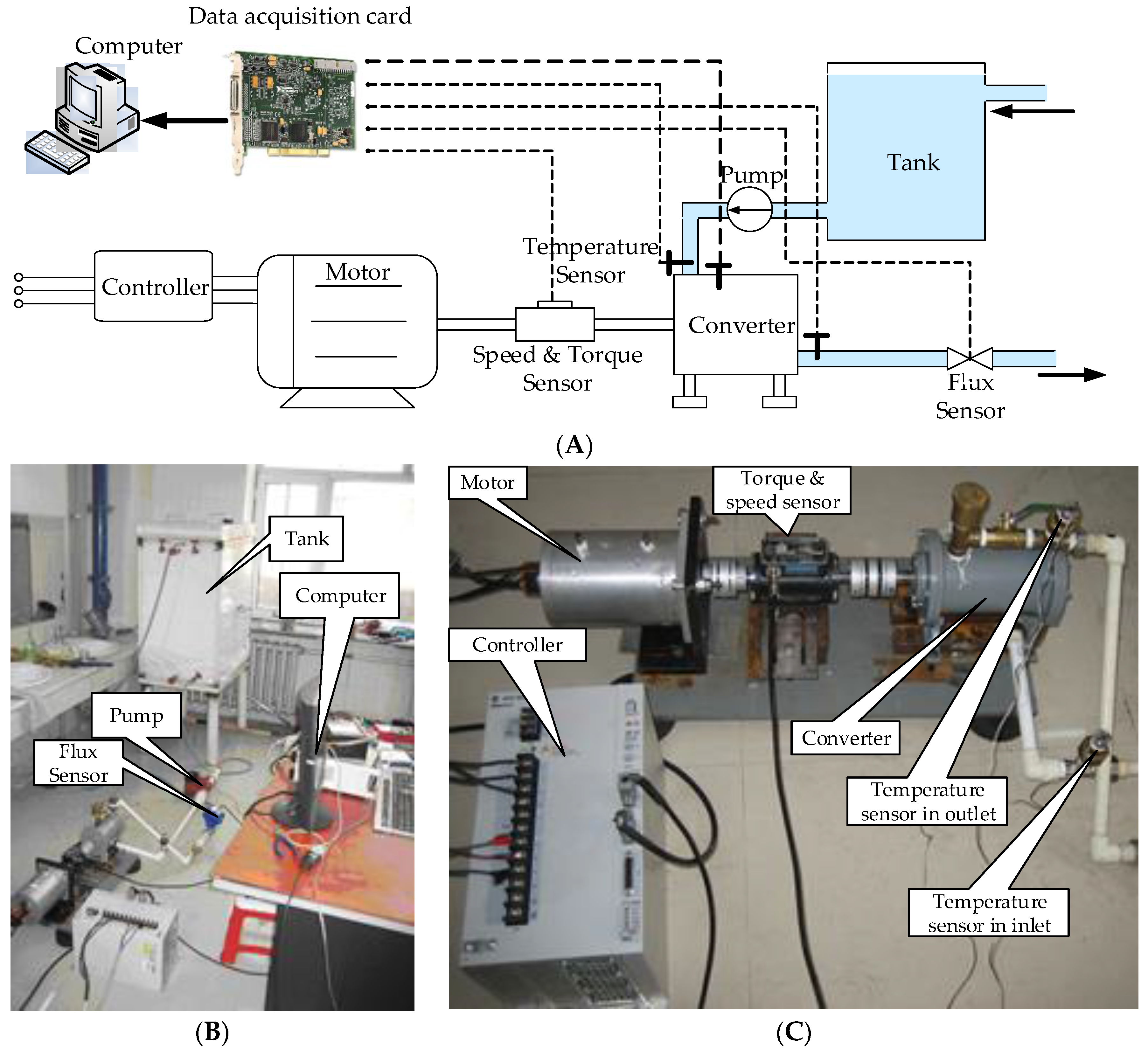
5. Experiments
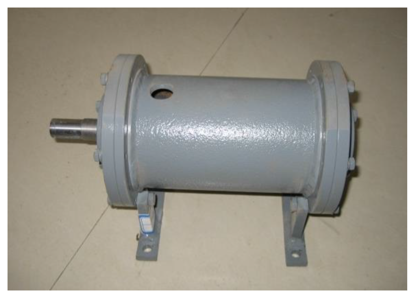
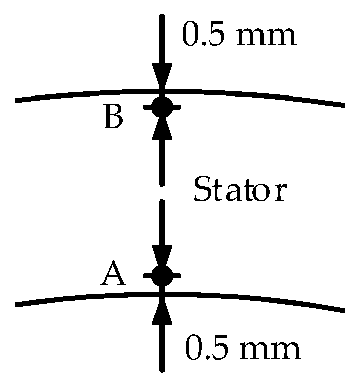
5.1. Experimental System
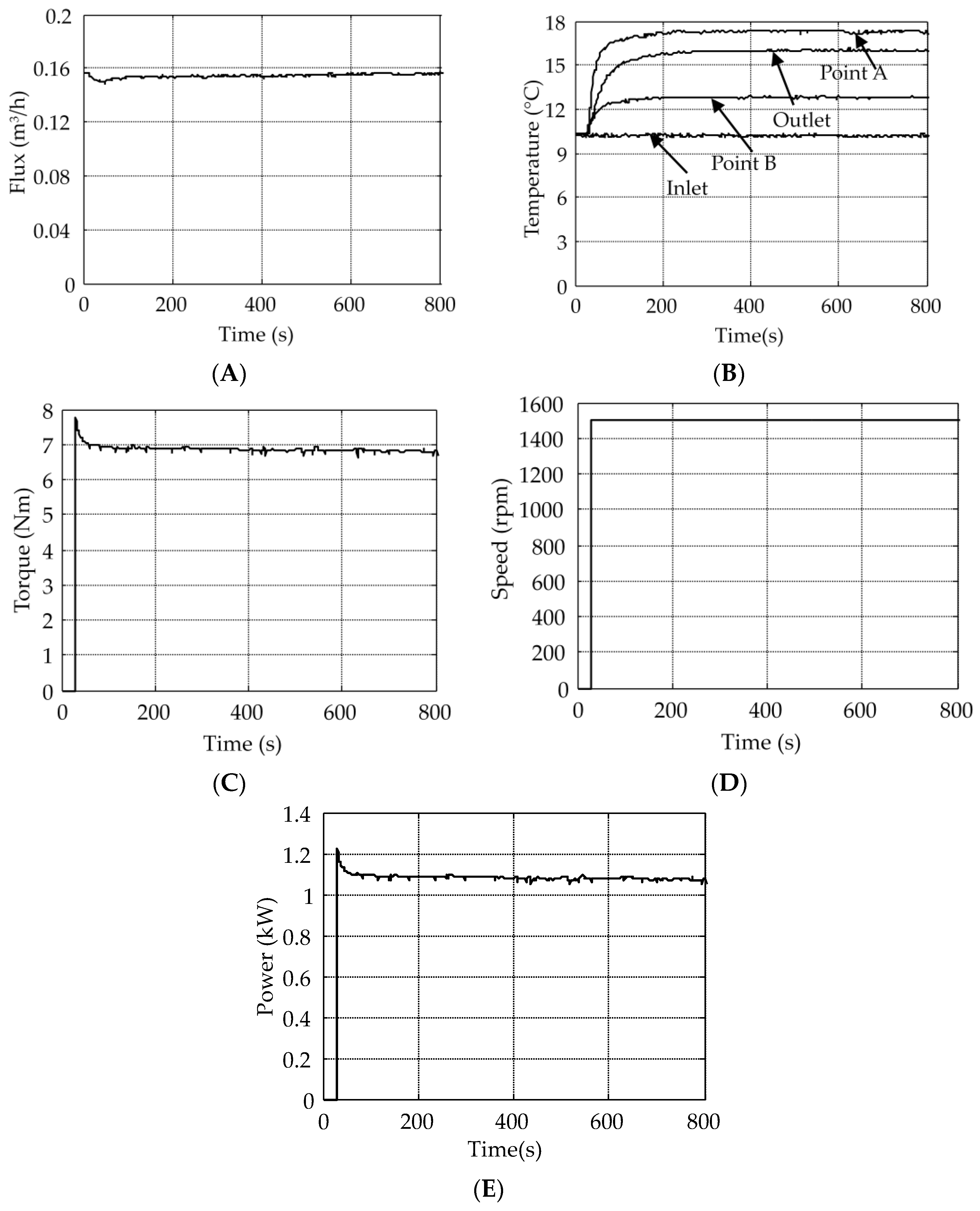
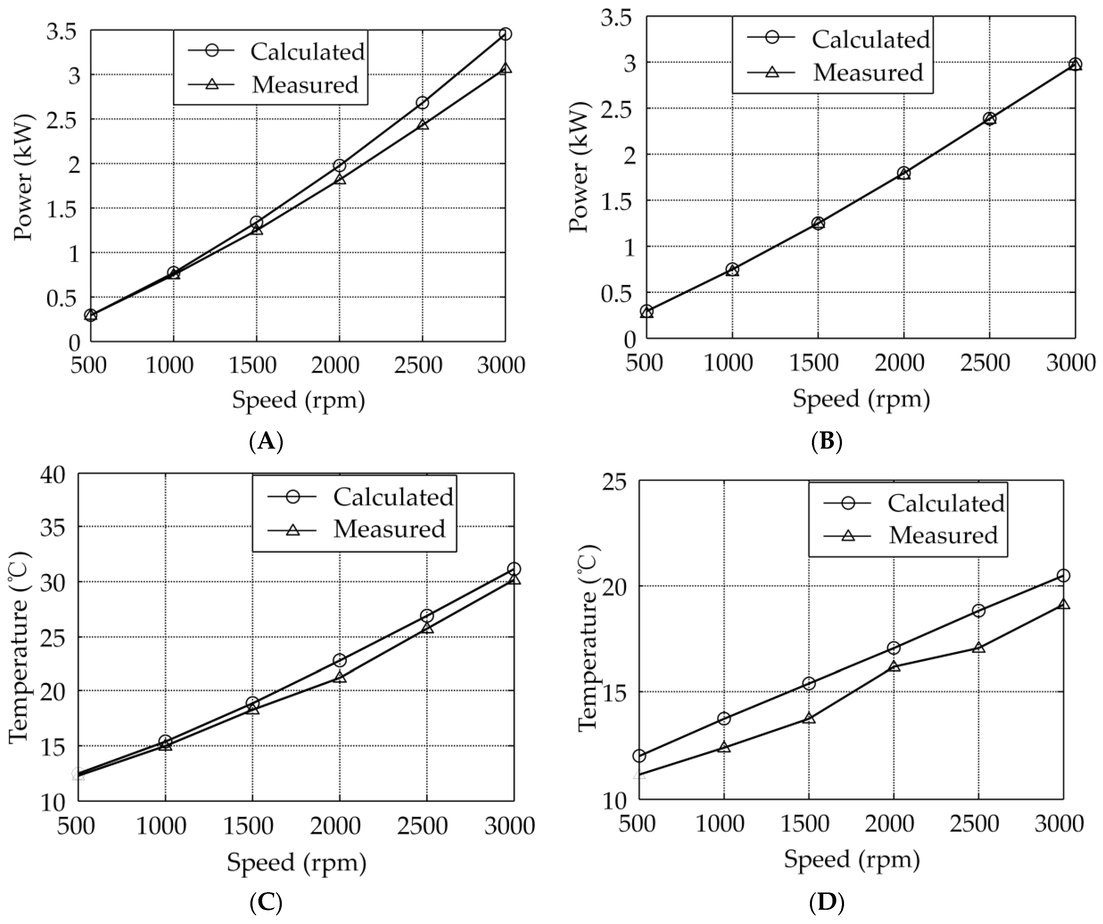
5.2. Results and Discussion
6. Conclusions
Acknowledgments
Author Contributions
Conflicts of Interest
References
- Oh, J.-H.; Nam, Y. Study on the Effect of Ground Heat Storage by Solar. Heat Using Numerical Simulation. Energies 2015, 8, 13609–13627. [Google Scholar] [CrossRef]
- International Energy Agency (IEA). World Energy Outlook 2013; IEA: Paris, France, 2013. [Google Scholar]
- Moretti, E.; Bonamente, E.; Buratti, C.; Cotana, F. Development of Innovative Heating and Cooling Systems Using Renewable Energy Sources for Non-Residential Buildings. Energies 2013, 6, 5114–5129. [Google Scholar] [CrossRef]
- Tchapda, A.H.; Pisupati, S.V. A Review of Thermal Co-Conversion of Coal and Biomass/Waste. Energies 2014, 7, 1098–1148. [Google Scholar] [CrossRef]
- Valanciusemail, R.; Jurelionis, A.; Dorosevas, V. Method for cost-benefit analysis of improved indoor climate conditions and reduced energy consumption in office buildings. Energies 2013, 6, 4591–4606. [Google Scholar] [CrossRef]
- Pisello, A.L.; Cotana, F.; Nicolini, A.; Brinchi, L. Development of clay tile coatings for steep-sloped cool roofs. Energies 2013, 6, 3637–3653. [Google Scholar] [CrossRef]
- Buratti, C.; Moretti, E. Glazing systems with silica aerogel for energy savings in buildings. Appl. Energy 2012, 98, 396–403. [Google Scholar] [CrossRef]
- Agemar, T.; Weber, J.; Schulz, R. Deep Geothermal Energy Production in Germany. Energies 2014, 7, 4397–4416. [Google Scholar] [CrossRef]
- Cheng, M.; Sun, L.; Buja, G.; Song, L. Advanced Electrical Machines and Machine-Based Systems for Electric and Hybrid Vehicles. Energies 2015, 8, 9541–9564. [Google Scholar] [CrossRef]
- Chu, W.Q.; Zhu, Z.Q.; Liu, X.; Stone, D.A.; Foster, M.P. Iron loss calculation in permanent magnet machines under unconventional operations. IEEE Trans. Magn. 2014, 50, 1–4. [Google Scholar] [CrossRef]
- Zhao, J.; Liu, W.; Li, B.; Liu, X.; Gao, C.; Gu, Z. Investigation of Electromagnetic, Thermal and Mechanical Characteristics of a Five-Phase Dual-Rotor Permanent-Magnet Synchronous Motor. Energies 2015, 8, 9688–9718. [Google Scholar] [CrossRef]
- Choi, J.; Kim, S.-K.; Kim, K.; Park, M.; Yu, I.-K.; Kim, S.; Sim, K. Design and Performance Evaluation of a Multi-Purpose HTS DC Induction Heating Machine for Industrial Applications. IEEE Trans. Appl. Supercond. 2015, 25, 1–5. [Google Scholar] [CrossRef]
- Araneo, R.; Dughiero, F.; Fabbri, M.; Forzan, M.; Geri, A.; Morandi, A.; Lupi, S.; Ribani, P.L.; Veca, G. Electromagnetic and thermal analysis of the induction heating of aluminum billets rotating in DC magnetic field. COMPEL 2008, 27, 467–479. [Google Scholar]
- Fabbri, M.; Morandi, A.; Negrini, F. Temperature Distribution in Aluminum Billets Heated by Rotation in Static Magnetic Feld Produced by Superconducting Magnets. COMPEL 2005, 24, 281–290. [Google Scholar] [CrossRef]
- Fabbri, M.; Morandi, A.; Ribani, P.L. DC Induction Heating of Aluminum Billets Using Superconducting Magnets. COMPEL 2008, 27, 480–490. [Google Scholar]
- Fabbri, M.; Forzan, M.; Lupi, S.; Morandi, A.; Ribani, P.L. Experimental and Numerical Analysis of DC Induction Heating of Aluminum Billets. IEEE Trans. Magn. 2009, 45, 192–200. [Google Scholar] [CrossRef]
- Magnusson, N.; Bersås, R.; Runde, M. Induction Heating of Aluminum Billets Using HTS DC Coils. Inst. Phys. Conf. Ser. 2004, 181, 1104–1109. [Google Scholar]
- Morandi, A.; Fabbri, M.; Ribani, P.L. Design of a Superconducting Saddle Magnet for DC Induction Heating of Aluminum Billets. IEEE Trans. Appl. Supercond. 2008, 18, 816–819. [Google Scholar] [CrossRef]
- Lubin, T.; Netter, D.; Leveque, J.; Rezzoug, A. Induction Heating of Aluminum Billets Subjected to a Strong Rotating Magnetic Field Produced by Superconducting Windings. IEEE Trans. Magn. 2009, 45, 2118–2127. [Google Scholar] [CrossRef]
- Watanabe, T.; Todaka, T.; Enokizono, M. Analysis of a New Induction Heating Device by Using Permanent Magnets. IEEE Trans. Magn. 2005, 41, 1884–1887. [Google Scholar] [CrossRef]
- Dabala, K. Analysis of mechanical losses in three-phase squirrel-cage induction motors. In Proceedings of the Fifth International Conference on Electrical Machines and Systems (ICEMS 2001), Shenyang, China, 18–20 August 2001.
- Lei, C.; Feng, C.; Yulong, P.; Shukang, C. The Solution of the 3D Electromagnetic Equation and Research on Related Electromagnetic Parameters of the Novel Rotational Electromagnetic Heating Machine. Trans. China Electrotechn. Soc. 2011, 26, 147–153. [Google Scholar]
- Huppunen, J. High-Speed Solid-Rotor Induction Machine Electromagnetic Calculation and Design. Ph.D. Thesis, Lappeenranta University of Technology, Lappeenranta, Finland, 3 December 2004. [Google Scholar]
- Zhu, Z.Q.; Ng, K.; Schofield, N.; Howe, D. Improved Analytical Modeling of Rotor Eddy Current loss in Brushless Machines Equipped with Surface Mounted Permanent Magnets. IEE Proc. Elect Power Appl. 2004, 151, 641–650. [Google Scholar] [CrossRef]
- Stranges, N. An Investigation of Iron Losses Due to Rotating Flux in Three Phase Induction Motor Cores. Ph.D. Thesis, McMaster University, Hamilton, ON, Canada, 2000. [Google Scholar]
- Shikun, C. Design of Electrical Machines; China Machine Press: Beijing, China, 2002; pp. 76–77. [Google Scholar]
- Ionel, D.M.; Popescu, M.; Dellinger, S.J. On the Variation with Flux and Frequency of the Core Loss Coefficients in Electrical Machines. IEEE Trans. Magn. 2006, 42, 658–667. [Google Scholar] [CrossRef]
- Ravnik, J.; Hriberšek, M.; Škerget, L. Coupled BEM–FEM analysis of flow and heat transfer over a solar thermal collector. Eng. Anal. Bound. Elem. 2014, 45, 20–28. [Google Scholar] [CrossRef]
- Ishak, D.; Zhu, Z.Q.; Howe, D. Eddy Current Loss in the Rotor Magnets of Permanent-magnets Brushless Machines Having a Fractional Number of Slots per Pole. IEEE Trans. Magn. 2005, 41, 2462–2469. [Google Scholar] [CrossRef]


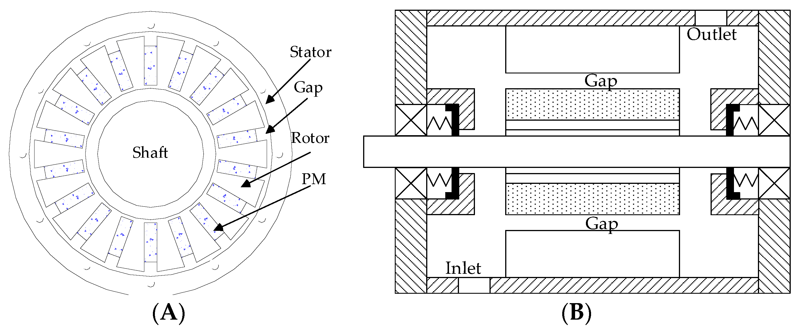
| Parameters | Dimensions | Materials |
|---|---|---|
| Stator outer diameter | 70 mm | Steel 20# |
| Stator inner diameter | 58 mm | |
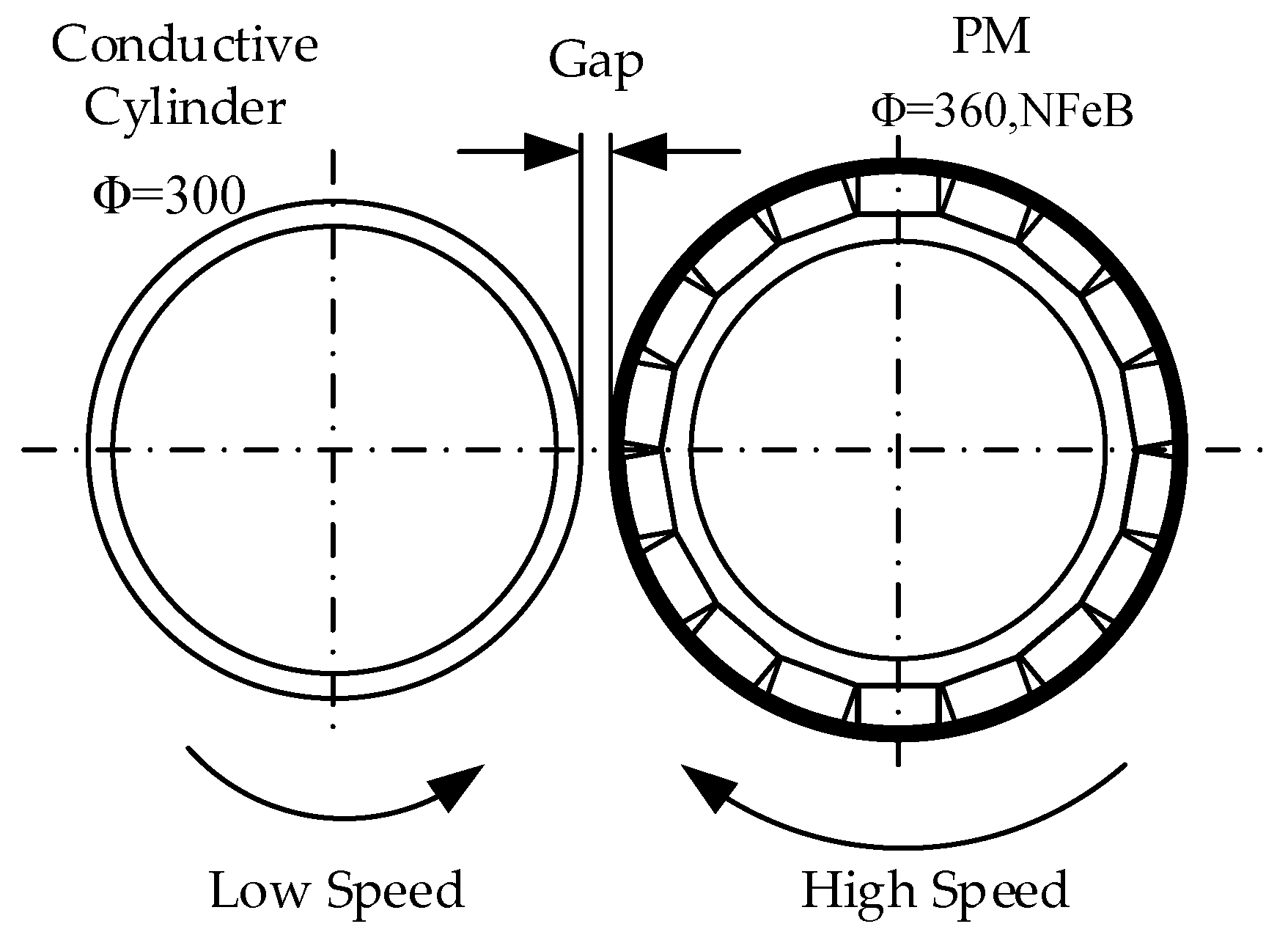
| Gap length | 0.3 mm | N/A |
| Rotor outer diameter | 57.4 mm | Steel 20# |
| Pole pairs | 9 | N/A |
| PM magnetization length | 3 mm | N33μH |
| PM width | 10 mm | |
| Axial length | 55 mm | N/A |
© 2016 by the authors; licensee MDPI, Basel, Switzerland. This article is an open access article distributed under the terms and conditions of the Creative Commons Attribution (CC-BY) license (http://creativecommons.org/licenses/by/4.0/).
Share and Cite
Chen, L.; Pei, Y.; Chai, F.; Cheng, S. Investigation of a Novel Mechanical to Thermal Energy Converter Based on the Inverse Problem of Electric Machines. Energies 2016, 9, 518. https://doi.org/10.3390/en9070518
Chen L, Pei Y, Chai F, Cheng S. Investigation of a Novel Mechanical to Thermal Energy Converter Based on the Inverse Problem of Electric Machines. Energies. 2016; 9(7):518. https://doi.org/10.3390/en9070518
Chicago/Turabian StyleChen, Lei, Yulong Pei, Feng Chai, and Shukang Cheng. 2016. "Investigation of a Novel Mechanical to Thermal Energy Converter Based on the Inverse Problem of Electric Machines" Energies 9, no. 7: 518. https://doi.org/10.3390/en9070518