Scheduling of Electricity Storage for Peak Shaving with Minimal Device Wear

Abstract

In this work, we investigate scheduling problems for electrical energy storage systems and formulate an algorithm that finds an optimal solution with minimal charging cycles in the case of a single device. For the considered problems, the storage system is used to reduce the peaks of the production and consumption within (part of) the electricity distribution grid, while minimizing device wear. The presented mathematical model of the storage systems captures the general characteristic of electrical energy storage devices while omitting the details of the specific technology used to store the energy. In this way, the model can be applied to a wide range of settings. Within the model, the wear of the storage devices is modeled by either: (1) the total energy throughput; or (2) the number of switches between charging and discharging, the so-called charging cycles. For the first case, where the energy throughput determines the device wear, a linear programming formulation is given. For the case where charging cycles are considered, an NP-hardness proof is given for instances with multiple storage devices. Furthermore, several observations about the structure of the problem are given when considering a single device. Using these observations, we develop a polynomial time algorithm of low complexity that determines an optimal solution. Furthermore, the solutions produced by this algorithm also minimize the throughput, next to the charging cycles, of the device. Due to the low complexity, the algorithm can be applied in various decentralized smart grid applications within future electricity distribution grids.

1. Introduction

Electricity distribution grids in the Western world have been changing rapidly over the last decade. Traditionally, a small number of large-scale power plants produced the power consumed by a large number of customers. This structure of the power distribution system implies that power flows unidirectionally from the large suppliers through the transmission and distribution grids towards the customers [1,2]. However, in recent years, large amounts of small-scale distributed generation are being introduced into the system at the customer level [3,4]. This shift from bulk generation at a few sites to both small-scale and local generation requires a different approach in thinking about, planning for and using our electricity distribution grid.

Local, small-scale generation units are often based on renewable sources, such as wind and sun. Their introduction is driven by environmental and sustainability targets, such as the 20-20-20 targets in the EU [2,5]. If a small number of these units is introduced in an area, the effect on the power flow within the area is negligible. However, a large penetration within an area may lead to larger, severe negative effects on the electricity distribution grid within the area. At specific times, the energy generated by the small-scale units may be far larger than the energy consumed. This results in a large, inverted power flow upstream to transport the power away to other areas where it can be consumed (see, e.g., [6]). Furthermore, our society is increasingly relying on electricity as a power source, as is clear from the introduction of, amongst other devices, heat pumps, electric stoves and electric vehicles (see, e.g., [7,8]). These devices tend to have a high simultaneity factor, causing high peak demand. However, our electricity distribution grids were not designed for these changes and need to be adapted in the future to accommodate such changes.

Electrical energy storage is seen as a viable option to address many of the challenges resulting from the recent changes in our electricity distribution grids (see, e.g., [9,10]). For example, an electrical energy storage system (EESS) is considered as one of the options to reduce the peaks in both supply and demand within distribution grids (see, e.g., [11,12,13]). Such a reduction of peaks leads to a reduced amount of stress on the network assets and by that increases their expected remaining lifetime. Furthermore, the need for costly grid reinforcements can be deferred through the use of an EESS to keep power flows within grid limitations. Finally, an EESS can be used to bridge the time gap between the generation of renewable energy and the desired time of use (see, e.g., [3,14]).

The potential positive effects of an EESS within the electricity distribution grid stimulated research within this area. For example, Johnson et al. [11] attempted to model and schedule an EESS to reduce maximum demand. Furthermore, Nykamp et al. [15] investigated the possibilities of an EESS to reduce the feed-in peaks of renewable energy sources based on data from Germany. Furthermore, Swierczynski et al. [16] demonstrated the capability of an EESS to operate on the Danish primary frequency regulation market. However, most of the current storage techniques are far from mature and are not economically feasible due to very high capital costs [10], except under rare conditions [6]. While prices are expected to drop in the future, as a result of technological advances, also the reduction of the wear of storage devices used within an EESS can greatly increase the number of economically feasible applications in the near future.

The many factors influencing the aging of a storage device are often captured by highly non-linear and linked relations, specifically in the case of batteries (see, e.g., [17,18]). Moreover, these relations are often dependent on the technology in question. Detailed modeling of the wear of an EESS thus leads to complex and hard to solve models. On the other hand, most applications of an EESS within an electricity distribution grid require fast control to cope with either real-time fluctuations in the power flow [16,19] or to ensure scalability to many concurrent systems [1]. Furthermore, as a large number of different storage devices are to be expected in the (future) grid, we pursue solutions that are applicable to many different systems. To this end, we model the general characteristics of energy storage device wearing and investigate the complexity of the obtained optimization models. While these models do not capture the full complexity of the aging of storage devices in all cases, we believe the results we obtain about the studied models form a suitable basis to be extended for more complex aging models.

While storage is often considered for grid balancing and peak shaving applications in the literature (see, e.g., [20,21,22]), device wearing is hardly considered. Koller et al. [23] do consider device wear in their storage models in the form of a mixed integer quadratic program, applicable within a model predictive control setting. However, they suggest to solve the problem via commercially available solvers, neglecting potential structural properties that can be exploited to construct a tailored and more efficient approach. Poullikkas et al. [24] investigate the economic potential of an EESS to defer conventional grid reinforcements on Cyprus. They claim to use a sophisticated model of the wearing, but no details are given. Haessig et al. [25] investigate the potential of an EESS to compensate for the fluctuating output of renewable energy sources. They limit wearing of the system in their models by restricting the number of full cycles. This constraint is shown to be equivalent with limiting the total throughput of the system. Our models differ in that we consider device wear in the objective instead of the constraints and that we also incorporate partial charging cycles. Wang et al. [26] consider a model for a hybrid system, exploiting storage devices of different technologies. Their formulation results in a convex optimization problem, without giving specifics on the complexity. Finally, Nykamp et al. [15] consider an EESS, in particular a battery, as an application to shave peaks of fluctuating renewable generation. They model the minimization of charging cycles as a mixed-integer linear program (MILP). We consider a similar problem, solving it using a tailored algorithm with complexity $O\left(N^3\right)$, where N is typically small in practice.

In this work, we study the complexity of optimization problems for scheduling the usage of an EESS. Within the model, the flattening of peaks within a given load profile is set up as a constraint. The objective is to minimize the aging of the storage devices in the system. As previously mentioned, the solutions to the considered problems should be fast and efficient. To ensure this, and to keep the model as general as possible, we concentrate on two common factors that influence the aging of storage devices: (1) the total throughput of the storage devices; and (2) the number of switches between charging and discharging made by the devices, the so-called charging cycles. The contributions of this work are as follows:

• We model the minimization of the storage degradation in the considered peak shaving method as a linear program (LP) when minimizing throughput, implying polynomial solvability.
• We model the problem as an MILP when minimizing charging cycles.
• We give an NP-hardness proof for the problem when minimizing charging cycles using multiple devices.
• We give several structural properties of an optimal solution that minimizes the number of charging cycles of a single device, which we use as a basis to construct a polynomial-time algorithm that minimizes both the number of charging cycles and the throughput of the devices.

The rest of this work is organized as follows. In the next section, a mathematical description of the considered setting and the associated optimization problems are given. Afterwards, in Section 3, the difference in the complexity status of the two considered objectives is discussed. This is followed in Section 4 by a study of the structure of the problem when the EESS consists of a single device. This results in a polynomial-time algorithm for this case. Then, in Section 5, we compare the obtained results for the two different objectives considered. Finally, in Section 6, some conclusions are drawn.

2. Model Description

In this section, we first give a short overview of the considered model, followed by a mathematical description of the associated optimization problem. We consider a given electricity distribution grid with an asset (e.g., a transformer or cable) for which an EESS is used to ensure the energy flows are within predetermined bounds. For this grid, we consider a given time horizon, which we assume is discretized into time intervals. For every time interval within the considered horizon, a prediction of the total energy flow through the asset, before use of an EESS, is given. Furthermore, within the model, bounds on these energy flow values through the asset are specified. The EESS now has to ensure that the remaining flow, after using the EESS, is between the given bounds for the time intervals.

The mathematical formulation of the optimization problem associated with the model sketched above is as follows. We consider a discrete time horizon given by a set of time intervals $\mathcal{T}=\{1,\dots ,T\}$. For each time interval $t\in \mathcal{T}$, we are given the flow value $F_t$, which we want to increase or decrease by using the EESS. For each time interval $t\in \mathcal{T}$, we are also given a lower bound $L{B}_t$ and an upper bound $U{B}_t$ on the resulting flow in time interval t. Furthermore, we consider the EESS as a set of storage devices, which are indexed by the set $\mathcal{U}=\{1,\dots ,I\}$. For each device $i\in \mathcal{U}$, three parameters are given: the (maximum) power $P_i$ of the device, the initial state of charge $So{C}_{i,0}$ and the maximum storage capacity $C_i$. The decision variables that control the use of the devices are given by the variables $s_{i,t}$ denoting the amount of energy that flows into or out of device i in time interval t. Note that negative values of $s_{i,t}$ mean that the device is discharging and extra energy is fed into the considered system. For each storage device, the total amount of energy stored inside the device at the end of time interval $t\in \mathcal{T}$ can be calculated by $So{C}_{i,t}:=So{C}_{i,0}+{\sum }_{j=1}^t{s}_{i,j}$. Note that we assume a perfect storage device, i.e., we assume the device has an efficiency of 100% when charging/discharging, to improve the readability of the work. The results in this work can be adapted in a straightforward manner to include lower efficiency levels. The choices for the decision variables are limited by the following constraints:

$$\begin{array}{ccc}& L{B}_t\le F_t-\sum _{i\in \mathcal{U}}{s}_{i,t}\le U{B}_t\hfill & \hfill \forall t\in \mathcal{T}\end{array}$$

(1)

$$\begin{array}{ccc}& -P_i\le s_{i,t}\le P_i\hfill & \hfill \forall t\in \mathcal{T}\forall i\in \mathcal{U}\end{array}$$

(2)

$$\begin{array}{ccc}& 0\le So{C}_{i,t}\le C_i\hfill & \hfill \forall t\in \mathcal{T}\forall i\in \mathcal{U}\end{array}$$

(3)

Constraints (1) ensure that the remaining flow after usage of the EESS is between the given bounds. These constraints can be rewritten to:

$$\begin{array}{ccc}& F_t-U{B}_t\le \sum _{i\in \mathcal{U}}{s}_{i,t}\le F_t-L{B}_t\hfill & \hfill \forall t\in \mathcal{T}\forall i\in \mathcal{U}\end{array}$$

(4)

which is somewhat easier to use later on. The second set of constraints (2) limits the (dis)charging done by each device by its given power. Finally, constraints (3) ensure that the energy stored in each device is always between zero and the capacity $C_i$ of the device. We note that further, linearized constraints imposed by the grid can be incorporated in the formulation.

To complete the formulation of the optimization model, it remains to define the optimization objective. Since the goal is to minimize device wear, this wearing needs to be expressed in terms of the variables in the model. The most straightforward option is to consider the total usage of the devices. This is given by the total amount of energy flowing in and out of each device over all time intervals, which is given by ${\sum }_{t\in \mathcal{T}}|s_{i,t}|$. As a result, we obtain the following optimization problem, which we call the $minThroughput$ problem:

$$\begin{array}{cc}& min\sum _{i\in \mathcal{U}}\sum _{t\in \mathcal{T}}|s_{i,t}|\hfill \\ & \text{s}.\text{t}.\left(1\right) – \left(3\right)\hfill \end{array}$$

(5)

However, for many storage devices, specifically batteries, the lifetime is generally expressed in charging cycles. A charging cycle is a time period in which the device switches once from charging to discharging and back to charging again, ignoring idle periods in between. The time before a storage device is assumed to have degraded too much is generally given by the manufacturer in full cycles, i.e., cycles in which the device goes from the full state of charge to complete empty and back to full at a constant (dis)charge rate (see, e.g., [27,28]). However, in real-time operation, most charging cycles do not fully discharge the storage device during every cycle. To take this into account, the notion of counting equivalent full cycles is sometimes used. An equivalent full cycle occurs over a set of time intervals if an amount of energy equal to the capacity has been both charged into and discharged from the device. We note that this is equivalent to considering the total throughput as an energy flow through the battery of twice the capacity to be then equivalent to one full cycle [25]. In contrast, in this work, we explicitly consider the minimization of the (partial) charging cycles, similar to Nykamp et al. [15]. By doing this, we enforce the considered devices in the EESS to prefer (near) full charging cycles over frequent charging cycles with small total throughput. This allows an effective estimation of the degradation and remaining life time of the considered devices by comparison with the given life time in full cycles as specified by the manufacturer. Furthermore, it prevents several forms of behavior that are considered damaging for several types of storage devices, such as frequent cycling at a low state of charge (see, e.g., [17,26]).

To integrate charging cycles into the model, we introduce two more sets of variables:

$$\begin{array}{ccc}\hfill X_{i,t}& =\left\{\begin{array}{cc}1\hfill & \text{if}{s}_{i,t}>0\hfill \\ 1\hfill & \text{if}{s}_{i,t}=0\text{and}{X}_{i,t-1}=1\hfill \\ 0\hfill & \text{if}{s}_{i,t}<0\hfill \\ 0\hfill & \text{if}{s}_{i,t}=0\text{and}{X}_{i,t-1}=0\hfill \end{array}\right.\hfill & \hfill \forall t\in \mathcal{T}\forall i\in \mathcal{U}\end{array}$$

(6)

$$\begin{array}{ccc}\hfill Y_{i,t}& =|X_{i,t}-X_{i,t-1}|\hfill & \hfill \forall t\in \mathcal{T}\forall i\in \mathcal{U}\end{array}$$

(7)

Note that $X_{i,t}$ indicates if device i is charging or discharging during time interval t, whereby the previous state is used in case the device is idle. Furthermore, $X_{i,0}$ is an input parameter indicating if device i had been charging or discharging before the start of the time horizon. The resulting binary variables $Y_{i,t}$ indicate if a switch between charging and discharging or vice versa occurred for device i between time intervals $t-1$ and t. An example of a flow of energy into and from a device with $X_{i,0}=0$ and with corresponding values of $X_{i,t}$ and $Y_{i,t}$ is given in Figure 1. Note that a charging cycle is defined as exactly two such switches, thus minimizing the number of charging cycles is equivalent to minimizing the number of switches. The resulting optimization problem, which we term $minCC$, is thus given by:

$$\begin{array}{cc}& min\sum _{i\in \mathcal{U}}\sum _{t\in \mathcal{T}}{Y}_{i,t}\hfill \\ & \text{s}.\text{t}.\left(1\right) – \left(3\right),\left(6\right)\text{ and }\left(7\right)\hfill \end{array}$$

(8)

3. Complexity Results

In this section, we investigate the complexity state of the problems introduced in the previous section. We begin by noting that we can split the variables $s_{i,t}$ into their positive and negative parts (i.e., $s_{i,t}=s_{i,t}^{+}-s_{i,t}^{-}$ with $s_{i,t}^{+},s_{i,t}^{-}\ge 0$). After this reformulation, the $minThroughput$ problem (5) becomes an LP. Thus, this problem can be solved in polynomial time and is therefore in general easy to solve. The complexity state of problem $minCC$ is not as straightforward, as the use of the binary variables $X_{i,t}$ and $Y_{i,t}$ suggest that the problem might be difficult to solve. In fact, this problem is hard.

Theorem 1. 

Problem $minCC$ is NP-hard for multiple devices ($I\ge 2$) and NP-hard in the strong sense if the number of devices I is part of the input. This result also holds when all devices are assumed to be equal.

Proof. 

We use reductions from the classical NP-complete problems three-partition and partition (see, e.g., [29]). We begin by reformulating $minCC$ into a decision problem by replacing the minimization objective with the question if there exists a feasible solution with ${\sum }_{i\in \mathcal{U}}{\sum }_{t\in \mathcal{T}}{Y}_{i,t}\le K$ for some parameter K. Note that the reformulation is in NP because it is straightforward to compute the number of switches for any given schedule for each device in time linear in the length of the scheduling horizon T. Then we reduce the three-partition problem to our decision problem, and as three-partition is NP-complete in the strong sense, so our problem is.

Consider an instance of the three-partition problem. Given is a (multi)set $X=\{x_1,x_2,\dots ,x_{3m}\}$ of positive integers with ${\sum }_{i=1}^{3m}{x}_i=mB$ and $B/4<x_i<B/2,i=1,\dots ,3m$. The three-partition problem asks if there exist sets $X_1,X_2,\dots ,X_m$ partitioning X, such that ${\sum }_{x_i\in X_k}{x}_i=B,k=1,\dots ,m$. A corresponding instance of $minCC$ is then constructed by taking:

• $T=6m+1$
• $I=m$
• $P_i=B,\forall i\in \mathcal{U}$
• $C_i=3mB,\forall i\in \mathcal{U}$
• $So{C}_{i,0}=0\forall i\in \mathcal{U}$
• $U{B}_t=B$ and $L{B}_t=-\infty \forall t\in \mathcal{T}$
• $F_t=(m+1)B$ for $t=1,3,5,\dots ,6m+1$ and $F_t=B-x_{t/2}$ for $t=2,4,6,\dots ,6m$
• $K=6m$

An example of the constructed instance of $minCC$ for $m=3$ and the multiset of integers given by $\{1,2,3,4,4,5,5,6,6\}$ is given in Figure 2. For this instance, we get that $B=12,(m+1)B=48$ and $C_i=108$ for $i=1,2,3$. The light grey areas for the even time intervals indicate the potential to discharge some energy by the devices in those time intervals.

Assume the constructed instance of the decision variant of $minCC$ is a yes-instance. Note that $F_t=(m+1)B$ and $U{B}_t=B$ for the odd time intervals and furthermore $P_i=B$ for all $i\in \mathcal{U}$. Thus, every device needs to charge B units of energy on every odd time interval, resulting in a total of $B(3m+1)$ units charged into every device over the whole time horizon. Thus, since $C_i=3mB$, every device needs to discharge at least B units of energy on the even time intervals. Since $U{B}_t=B$ and $F_t=B-x_{t/2},t=2,4,\dots ,6m$, the maximum amount that can be discharged on these even time intervals is ${\sum }_{t=1}^{3m}{x}_t=mB$. From this, it follows that each device discharges exactly B over the whole time horizon. It also follows that the devices together discharge $x_{t/2}$ units of energy on every even time interval t, meaning that at least one device is discharging on every even time interval. Furthermore, whenever a device is discharging on any of the even time intervals, this induces two switches. Thus, since $K=6m$ and $T=6m+1$, there has to be exactly one device discharging on each of the even time intervals. Thus, each device discharges the amount needed for a subset $X_i$ of the even time intervals with a total load of B. Together, these sets $X_i$ form the partition of X.

Now, assume that the instance of the three-partition is a yes-instance. Then, taking $s_{i,t}=B$ for t odd, $s_{i,t}=-x_{t/2}$ for t even whenever $x_{t/2}\in X_i$ and $s_{i,t}=0$ otherwise is a solution to the decision variant of $minCC$.

Note that the number of devices in the given reduction is taken as an input parameter, while in many applications, the number of devices is fixed. For the case of only two devices, a reduction from the partition problem to $minCC$ can be done in a similar way as above. Hereby, both devices are forced to charge B units more than their capacity. This gives a freedom of $s_i$ units to discharge on the even numbered time intervals. Limiting the number of switches again ensures only one device discharges on each of the even numbered time intervals. This results in a partition of the $s_i$’s over two sets.

In conclusion, we have that $minCC$ is NP-hard in the strong sense when the number of devices is an input parameter and NP-hard in the weak sense when the number of devices is fixed and larger than or equal to two.   ☐

4. Minimization of Charging Cycles for a Single Device

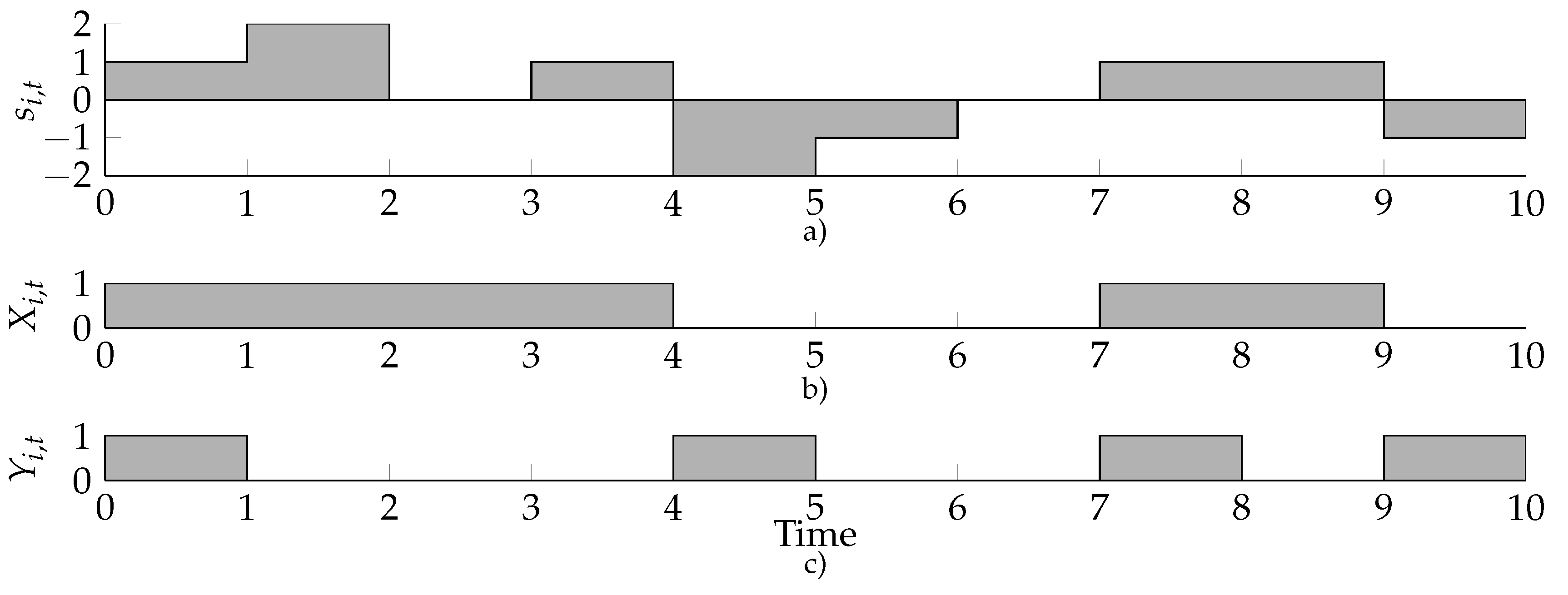
As we have seen in the previous section, the problem of minimizing the number of charging cycles when multiple devices are considered is difficult, even if all of the devices are equal and we do not incorporate any grid constraints beyond (1). However, finding a feasible solution and minimizing the throughput is easy, as it can be formulated as an LP. The question remains what happens when we consider minimizing charging cycles for a single device, i.e., when we consider the $minCC$ problem with $I=1$. We note that we omit further grid constraints beyond (1), since we can assume the storage device to be positioned reasonably close to the asset for which it is used to ensure the energy flow is between pre-specified bounds.

To tackle this problem, we first introduce some key observations in the next subsection followed by an optimal polynomial time algorithm in Subsection 4.2. As from here on we only consider a single storage device, the index i in the various variables and constraints will be omitted for readability.

4.1. Key Observations

When considering a single device, it is possible to combine the flow and power constraints (2) and (4). From (2), it follows that $s_t\in [-P,P]$, and from (4), it follows that $s_t\in [F_t-U{B}_t,F_t-L{B}_t]$. This gives us that $s_t$ must lie in the intersection of the two intervals for every t. If we define $A_t=max[F_t-U{B}_t,-P]$ and $B_t=min[F_t-L{B}_t,P]$, then the power and flow constraints (2) and (4) are equivalent to:

$$\begin{array}{ccc}& A_t\le s_t\le B_t\hfill & \hfill \forall t\in \mathcal{T}\end{array}$$

(9)

Note that it is possible that $A_t>B_t$ for some time interval if for example $F_t-U{B}_t>P$. However, this implies that the storage device cannot charge enough energy in a single time interval to get the resulting flow between the desired bounds. Since these instances are infeasible, we assume that this is never the case, i.e., we assume that $A_t\le B_t$ for all $t\in \mathcal{T}$.

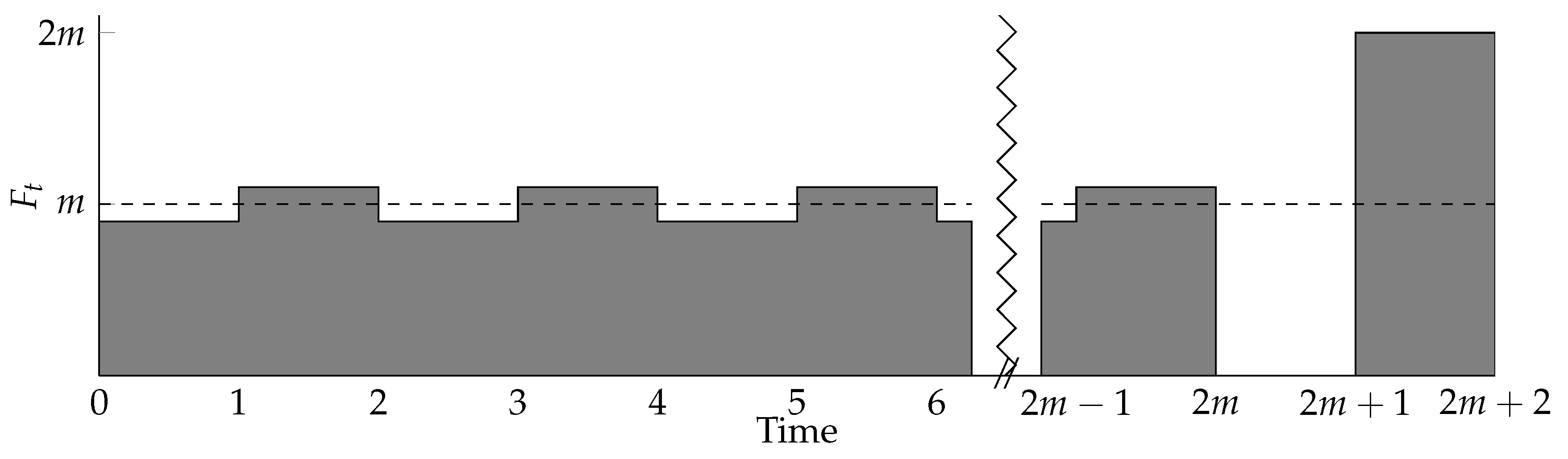
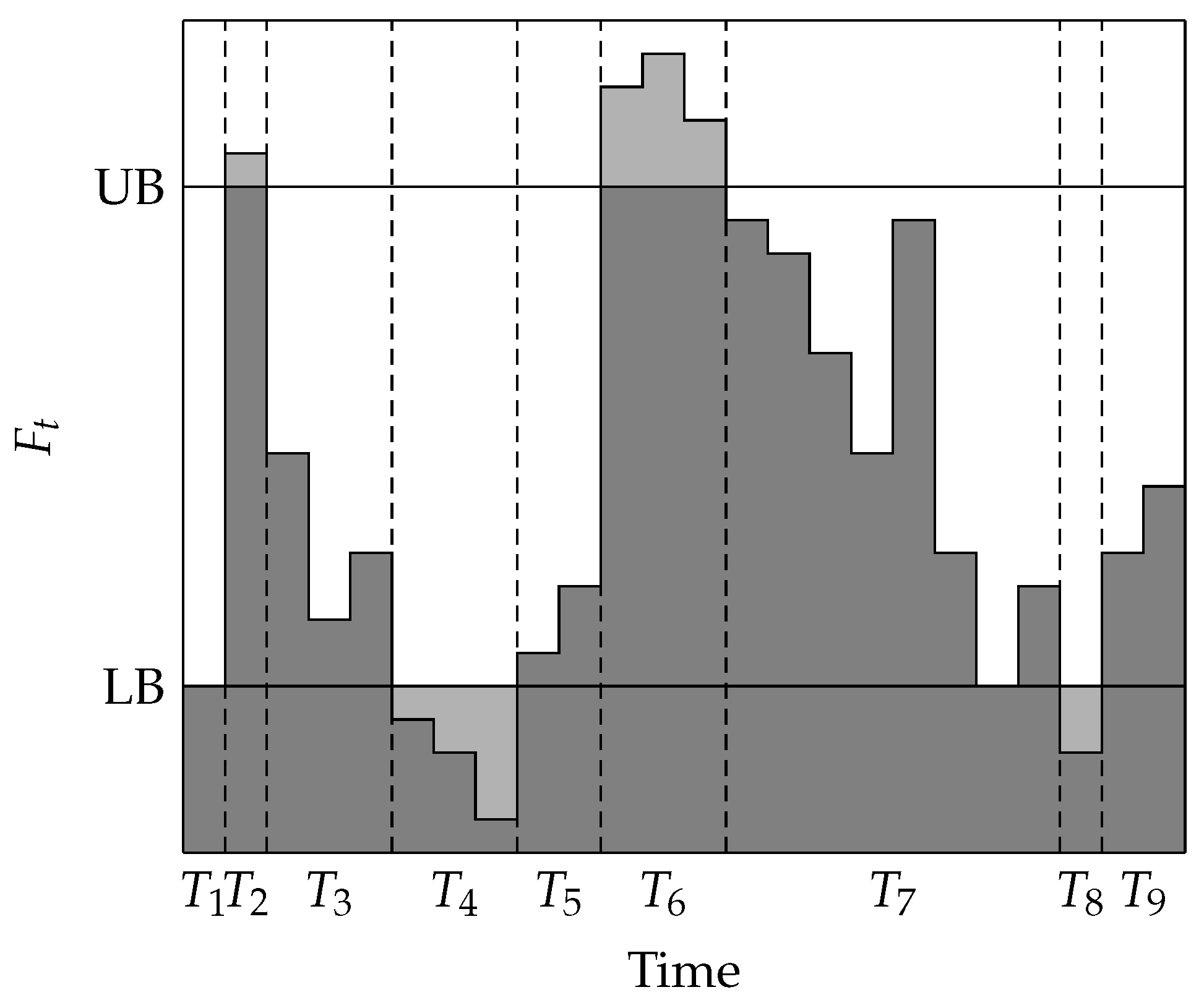
Let us now consider the set $\mathcal{T}$ of time intervals. We can characterize these time interval based on their intervals $[A_t,B_t]$ specifying the domain of $s_t$. We consider three possible options: (A) the device is not forced to do anything by the flow bounds (9); (B) the device is forced to charge by the flow bounds (9) and (C) the device is forced to discharge by the flow bounds (9). In the first case, we have that $0\in [A_t,B_t]$; in the second case, we have $A_t>0$; and in the last case, we have that $B_t<0$. If two consecutive time intervals t and $t+1$ both belong to Case (B), then in any feasible schedule, we have $s_t,s_{t+1}>0$. Furthermore, if t and $t-1$ belong to Case (C) then in any feasible schedule, we have $s_t,s_{t-1}<0$.

Now, assume that t and $t-1$ both belong to Case (A), and we have a feasible schedule with $s_t<0$ and $s_{t+1}>0$ or vice versa. Taking the smallest, in absolute value, of the two values and adding it to the other results in a feasible schedule that has either $s_t,s_{t+1}\ge 0$ or $s_t,s_{t+1}\le 0$. Note that this new schedule potentially has one switch less, but never more switches than the former schedule. Thus, we can restrict without loss of generality to schedules for which consecutive intervals that belong to the same case, as specified above, either both charge or both discharge. Hereby, we assume that doing nothing (i.e., $s_t=0$) can be seen as either charging or discharging.

The above property gives rise to a different way of approaching the set $\mathcal{T}$. Instead of considering the time intervals in $\mathcal{T}$ individually, it is possible to group them into blocks of consecutive time intervals with the same characteristic. These blocks form a partition of $\mathcal{T}$ and should be taken maximally with respect to the union, i.e., no two consecutive blocks should contain time intervals of the same characteristic. Let $T_1,T_2,\dots ,T_N$ be the resulting partition of $\mathcal{T}$ into blocks of the same characteristic. We say $T_m<T_n$ to indicate that $m<n$, which means that all time intervals in $T_m$ lie before the time intervals in $T_n$. An example of the partition of the time intervals into blocks is given in Figure 3.

It is now possible to reformulate $minCC$ in terms of blocks instead of time intervals. For readability, the variables and parameters corresponding to block $T_n$ will be denoted by index n. First, we consider the combined flow and power constraint (9). Defining $A_n:={\sum }_{t\in T_n}{A}_t$ and $B_n:={\sum }_{t\in T_n}{B}_t$ allows us to rewrite (9) as:

$$\begin{array}{ccc}& A_n\le s_n\le B_n\hfill & \hfill \text{for}n=1,2,\dots ,N\end{array}$$

(10)

Furthermore, the state of charge (SoC) of the device at the end of block $T_n$ is given by $So{C}_n:=So{C}_0+{\sum }_{n^{\prime }=1}^n{s}_{n^{\prime }}$. The SoC constraints (3) can then be rewritten as:

$$\begin{array}{ccc}& 0\le So{C}_n\le C\hfill & \hfill \text{for}n=1,2,\dots ,N\end{array}$$

(11)

A reformulation of (6) and (7) leads to:

$$\begin{array}{ccc}\hfill X_n& =\left\{\begin{array}{cc}1\hfill & \text{if}{s}_n>0\hfill \\ 1\hfill & \text{if}{s}_n=0\text{and}{X}_{n-1}=1\hfill \\ 0\hfill & \text{if}{s}_n<0\hfill \\ 0\hfill & \text{if}{s}_n=0\text{and}{X}_{n-1}=0\hfill \end{array}\right.\hfill & \hfill \text{for}n=1,2,\dots ,N\end{array}$$

(12)

$$\begin{array}{ccc}\hfill Y_n& =|X_n-X_{n-1}|\hfill & \hfill \text{for}n=1,2,\dots ,N\end{array}$$

(13)

Again, $X_0$ is an input parameter indicating if the device was charging or discharging at the beginning of the time horizon. The reformulation of $minCC$ then becomes:

$$\begin{array}{cc}& min\sum _{n=1}^N{Y}_n\hfill \\ & \text{s}.\text{t}.\left(10\right) – \left(13\right)\hfill \end{array}$$

(14)

By construction, we have that a feasible solution for this reformulation of $minCC$ can easily be transformed into a feasible solution of the original formulation of $minCC$ with the same objective value.

For solving $minCC$, the following simple, but specific schedule, which may be infeasible, plays an important role.

Definition 2. 

The naive local schedule $S^{na}$ is defined by:

$$s_n^{na}=\left\{\begin{array}{cc}0\hfill & \text{if}0\in [A_n,B_n]\hfill \\ A_n\hfill & \text{if}{A}_n>0\hfill \\ B_n\hfill & \text{if}{B}_n<0\hfill \end{array}\right.$$

(15)

Note that $S^{na}$ uses the device as little as possible while satisfying the flow and power constraints (10). However, it is possible that it violates the SoC constraints (11) at some point. Nevertheless, it can be used as a basis to construct a feasible (and optimal) schedule, as is shown below.

To deal with SoC-constraint violations, we make the following observation. Assume we have an infeasible schedule S with $So{C}_n<0$ for some block $T_n$. Furthermore assume that for some block $T_m<T_n$ we have $So{C}_m=C$. Updating S to become feasible requires that some extra energy is charged into the device before $T_n$. However, any extra energy charged before $T_m$ does not help, since it causes an overflow at $T_m$. Thus, any attempt to make S feasible has to charge an extra amount of $|So{C}_n|$ between blocks $T_m$ and $T_n$. This gives rise to the following definition:

Definition 3. 

For a given infeasible schedule S and block $T_n$ with either $So{C}_n<0$ or $So{C}_n>C$ in schedule S, the decoupling point is the last block $T_m$ before $T_n$ with $So{C}_m=C$ or $So{C}_m=0$, respectively.

These decoupling points indicate which blocks can be ignored when attempting to change an infeasible schedule to a feasible one. In the next subsection, structural properties are considered using the above observations, which lead to a polynomial time algorithm to solve the problem.

4.2. Algorithm

In this subsection, we consider the structure of the problem of minimizing the number of charging cycles of a single device. To tackle this problem, we first restrict ourselves to instances in which the naive local schedule $S^{na}$ drops below the zero state of charge only on the last block $T_N$ and never gets above the capacity C. The derived results for these specific instances form the base to solve the general case. Note, that in the restricted instances, $S^{na}$ satisfies the SoC constraints (11) for all blocks, but the last, by having $So{C}_N<0$. Furthermore, no feasible schedule can have fewer switches than $S^{na}$, since within $S^{na}$, the device is used as little as possible while satisfying (10). We first observe that feasible schedules that discharge differently than $S^{na}$ do not need to be considered.

Lemma 4. 

Any optimal schedule S for a restricted instance can be changed to a schedule with exactly the same discharging as $S^{na}$ while remaining optimal.

Proof. 

First, note that S cannot do less discharging on any block than $S^{na}$, since $S^{na}$ does the minimal discharging required to satisfy the flow and power constraints (10). Thus, assume S does some extra discharging over $S^{na}$. Let $T_n$ be the first block on which S does extra discharging, and let ${\Delta }_1$ be the difference between the discharging done by S and $S^{na}$ on $T_n$. Since S is feasible and $So{C}_N<0$ in $S^{na}$, this extra discharging must be compensated somewhere with extra charging. Let $T_m$ be the first block on which some extra charging is done compared to $S^{na}$, and let ${\Delta }_2$ be the difference between the amount of charging done by S and $S^{\prime }$ on $T_m$. Furthermore, let $S^{\prime }$ be the schedule obtained by canceling an amount of $\Delta :=min\{{\Delta }_1,{\Delta }_2\}$ extra discharging on $T_n$ and canceling an amount of Δ extra charging on $T_m$. Note that $s_n<s_n^{\prime }\le s_n^{na}$ and $s_m>s_m^{\prime }\ge s_m^{na}$, which implies that $S^{\prime }$ still satisfies the flow constraints (10). Furthermore, note that only the SoC of the blocks between $T_n$ and $T_m$ changes when obtaining schedule $S^{\prime }$ from S.

If $T_m<T_n$, then the SoC of each the blocks in between $T_m$ and $T_n$ decreases by Δ. However, the SoC of each of these blocks is bounded from below by their SoC in $S^{na}$ due to the minimality of n. Thus, it cannot drop below zero by the feasibility of $S^{na}$ for all blocks besides $T_N$. If on the other hand, $T_n<T_m$, the SoC of each block between $T_n$ and $T_m$ increases by Δ, but the SoC of each of these blocks is bounded from above by their SoC in S due to the minimality of m. Thus, it cannot rise above C by the feasibility of S.

The above argument can be repeated while there is at least one block on which more discharging is done by S than by $S^{na}$. Note that each update of S only cancels out some charging and discharging, which implies that the number of switches cannot increase while updating S. Thus, S remains optimal after the update. Finally, note that after each update in at least one extra block, the charging/discharging of S and $S^{na}$ coincide, which concludes the proof.   ☐

As a consequence of Lemma 4, for the considered restricted instances, we can take the naive local schedule $S^{na}$ as a basis and only add extra charging on some of the blocks. Since $S^{na}$ only discharges on blocks where it is required to do so by the flow and power constraints (10), the extra charging can only be done on blocks that are not used to discharge in $S^{na}$. However, not all of these blocks have the same potential for charging extra without violating either the flow and power constraints (10) or the SoC constraints (11). From the flow and power constraints (10), it follows that block $T_n$ cannot be used for more than $B_n-s_n$ extra charging. Furthermore, from the SoC constraints (11), it follows that the potential for extra charging of block $T_n$ is also limited by $C-So{C}_m$ for $n\le m\le N$. This leads to the following definition:

Definition 5. 

Given a schedule S and a block $T_n$, the potential for extra charging on $T_n$ in S, denoted by $M{C}_n\left(S\right)$, is given by $min\{B_n-s_n,C-So{C}_n,C-So{C}_{n+1},\dots ,C-So{C}_N\}$.

Clearly, only the blocks with $M{C}_n\left(S\right)>0$ are of interest for updating a given schedule S. Thus, the optimal schedule may be obtained from $S^{na}$ by iteratively doing an extra charging of at most $M{C}_n\left(S\right)$ units on block $T_n$. This is done until the SoC at block $T_N$ is exactly zero, to ensure optimality in a more general setting later on.

Let us consider the blocks on which extra charging is possible within a schedule S, i.e., those blocks with positive potential for extra charging. As by Lemma 4, we only have to consider schedules that do exactly the same discharging as $S^{na}$, this implies that any block in S that is used for discharging cannot have any potential for extra charging. This means that a block $T_n$ can only be used for extra charging in S if it is currently not used to discharge, i.e., if $s_n\ge 0$ in S. If a block is already used for charging, any extra charging done on this block does not increase the number of switches. Furthermore, any block $T_n$ that is unused in a schedule S (i.e., $s_n=0$) must also be unused in $S^{na}$, since by Lemma 4, for these blocks, we can only consider extra charging. By maximality of the blocks with respect to inclusion, it follows that both neighboring blocks $T_{n-1}$ and $T_{n+1}$ of an unused block $T_n$ must be used for either charging or discharging in $S^{na}$. Again, by Lemma 4, this implies that both $T_{n-1}$ and $T_{n+1}$ must be used for charging or discharging in S. Doing extra charging on $T_n$ in S now only causes two extra switches when both $T_{n-1}$ and $T_{n+1}$ are used for discharging. Note that in this case, any feasible schedule is discharging on both of these blocks.

Based on the above, we may partition the set of blocks that can be used for extra charging into two sets $\mathcal{P}\left(S\right)$ and $\mathcal{N}\left(S\right)$, those that cause extra switches when used for extra charging and those that do not:

$$\begin{array}{cc}\hfill \mathcal{P}\left(S\right)& =\left\{T_n\right|M{C}_n\left(S\right)>0,s_n=0,X_{n-1}=0,X_{n+1}=0\}\hfill \\ \hfill \mathcal{N}\left(S\right)& =\left\{T_n\right|M{C}_n\left(S\right)>0,T_n\notin \mathcal{P}\left(S\right)\}.\hfill \end{array}$$

Note that for any block $T_n$ used for discharging on schedule S, it holds that $M{C}_n\left(S\right)=0$, since by Lemma 4, we only consider extra charging over $S^{na}$. Thus, any block in $\mathcal{N}\left(S\right)$ must either be used for charging or has a neighboring block that is used for charging. In either case, any extra charging done on S cannot change this. Thus, any update to S by doing extra charging cannot cause a block in $\mathcal{N}\left(S\right)$ to become an element of $\mathcal{P}\left(S\right)$ instead. On the other hand, a block in $\mathcal{P}\left(S\right)$ can only become an element of $\mathcal{N}\left(S\right)$, if it is used for extra charging (without completely depleting its potential for extra charging).

As a consequence, the blocks in $\mathcal{N}\left(S^{na}\right)$ are preferred to be used over the blocks in $\mathcal{P}\left(S^{na}\right)$. In fact, it is always optimal to first use the blocks of $\mathcal{N}\left(S^{na}\right)$ to their maximal potential, as shown in the following lemma.

Lemma 6. 

Let S be a feasible schedule for a restricted instance, obtained from $S^{na}$ by doing some extra charging, and let $Z_{\mathcal{N}}$ and $Z_{\mathcal{P}}$ be the collections of blocks, from $\mathcal{N}\left(S^{na}\right)$ and $\mathcal{P}\left(S^{na}\right)$, respectively, which are used for extra charging. Furthermore, let $S^{\prime }$ be the schedule that is obtained from $S^{na}$ by only doing the extra charging of S on the blocks in $Z_{\mathcal{N}}$. Furthermore, assume $\mathcal{N}\left(S^{\prime }\right)\ne \varnothing$, and let $T_n$ be in $\mathcal{N}\left(S^{\prime }\right)$. Finally, let $T_m$ be the first block in $Z_{\mathcal{P}}$ and $\Delta >0$ the amount of extra charging done on $T_m$. Then, the schedule $S^{★}$ obtained from S by shifting ${\Delta }^{\prime }:=min\{\Delta ,M{C}_n\left(S^{\prime }\right)\}$ extra charging from $T_m$ to $T_n$ is also a feasible schedule with at most the same number of switches as S.

Proof. 

Let $S^{★}$ be the schedule obtained by the shift. First note that the shift of the extra charging between $T_m$ and $T_n$ cannot introduce a violation of the flow and power constraints (10). Furthermore, in $S^{★}$, the SoC is only changed for the blocks between $T_m$ and $T_n$ compared to S. First, assume that $T_m<T_n$. Then, the SoC of these blocks between $T_m$ and $T_n$ is decreased by ${\Delta }^{\prime }$. Since S and, thus, $S^{★}$ only does extra charging over $S^{na}$, it follows that the SoC of the blocks in between $T_m$ and $T_n$ in $S^{★}$ is bounded from below by the SoC of these blocks in $S^{na}$. Thus, the decrease in SoC cannot cause a drop of the SoC below zero. Next, assume that $T_n<T_m$. Then, the SoC of the blocks between $T_m$ and $T_n$ rises by ${\Delta }^{\prime }$. However, by construction, ${\Delta }^{\prime }\le M{C}_n\left(S^{\prime }\right)$, and all other blocks in $Z_{\mathcal{P}}$ lie after $T_m$. From this, it follows that the SoC of the blocks between $T_m$ and $T_n$ cannot increase above C. Finally, note that at most one extra block is used for extra charging in $S^{★}$ compared to S, but this block belongs to $\mathcal{N}\left(S^{na}\right)$; thus, no switches are introduced by the shift of charging from $T_m$ to $T_n$.   ☐

Lemma 6 shows that, while updating $S^{na}$ into a feasible schedule by extra charging on certain blocks, the blocks of $\mathcal{N}\left(S^{na}\right)$ can be preferred. However, as extra charging on some block can decrease the potential of other blocks, the question remains in what order the blocks from $\mathcal{N}\left(S^{na}\right)$ should be used for extra charging.

Lemma 7. 

Consider a restricted instance with a naive local schedule $S^{na}$. Then, exactly one of the following two cases holds: let S be any schedule obtained from $S^{na}$ by (only) extra charging on the blocks of $\mathcal{N}\left(S^{na}\right)$ for which $\mathcal{N}\left(S\right)=\varnothing$.

• There is a unique block $T_n$, such that it is the last block with $So{C}_n=C$ in any schedule S, that (only) does extra charging on blocks of $\mathcal{N}\left(S^{na}\right)$ and for which $\mathcal{N}\left(S\right)=\varnothing$. Furthermore, for any such schedule, all blocks $T_m\in \mathcal{N}\left(S^{na}\right)$ after $T_n$ have $s_m=B_m$.
• In any schedule S that (only) does extra charging on blocks of $\mathcal{N}\left(S^{na}\right)$ and for which $\mathcal{N}\left(S\right)=\varnothing$, all blocks $T_m\in \mathcal{N}\left(S^{na}\right)$ have $s_m=B_m$.

Proof. 

Let S be an arbitrary schedule that is obtained from $S^{na}$ by charging extra only on the blocks from $\mathcal{N}\left(S^{na}\right)$, such that $\mathcal{N}\left(S\right)=\varnothing$. Furthermore, assume that $So{C}_n<C$ for all blocks $T_n$ in schedule S. By assumption, it holds that $s_n=B_n$ for every block $T_n$ in S. Since $B_n$ is an upper bound for any block in any schedule, it follows that no block can reach an SoC of C for any schedule. Thus, if there is a single schedule for which the SoC never reaches C, then no schedule can reach an SoC of C.

It remains to show that, for schedules that reach an SoC of C for some block, the last block for which this occurs is the same. Let S and $S^{\prime }$ be two such schedules, and let $T_{n^{★}}$ and $T_{n^{\prime }}$ be the last block for which S, respectively $S^{\prime }$, reaches an SoC of C. Without loss of generality, let $T_{n^{★}}\le T_{n^{\prime }}$, and assume $T_{n^{★}}<T_{n^{\prime }}$. Since $So{C}_{n^{★}}=C$ on schedule S, $S^{\prime }$ cannot do more extra charging before $T_{n^{★}}$ than S does. Furthermore, note that $s_m=B_m$ for all blocks $T_m\in \mathcal{N}\left(S^{na}\right)$ with $T_m>T_{n^{★}}$, since $\mathcal{N}\left(S\right)=\varnothing$. Thus, for any block $T_m$ with $T_{n^{★}}\le T_m\le T_{n^{\prime }}$, it must hold that $s_m^{\prime }\le s_m$. From this, it follows that the total amount of extra charging done by $S^{\prime }$ before $T_{n^{\prime }}$ is bounded from above by the total amount of extra charging done by S before $T_{n^{\prime }}$. Thus, $So{C}_{n^{\prime }}$ is at least as high in S as it is in $S^{\prime }$. From this, it follows that $So{C}_{n^{\prime }}=C$ in S, which is a contradiction with the assumed maximality of $T_{n^{★}}$. Thus, it follows that $T_{n^{★}}=T_{n^{\prime }}$.   ☐

From Lemma 7, it follows that the blocks from $\mathcal{N}\left(S^{na}\right)$ that are used for extra charging can be picked in arbitrary order. The blocks in $\mathcal{P}\left(S^{na}\right)$, however, require some more consideration, since extra charging on one of those blocks adds two switches to the objective value. Thus, intuitively, it makes sense to consider the blocks that have the highest potential, which is in fact optimal, as shown in the following lemma.

Lemma 8. 

Let S be the schedule that is obtained from $S^{na}$ by iteratively doing extra charging on the blocks in $\mathcal{N}\left(S^{na}\right)$ until $\mathcal{N}\left(S\right)=\varnothing$. We define $S_0=S$ and iteratively construct a schedule $S_k$ for $k=1,2,\dots ,K$ as follows:

• Pick block T from $\mathcal{P}\left(S_{k-1}\right)$ with maximal $MC\left(S_{k-1}\right)$, and let $n\left(k\right)$ denote the index of this block.
• Construct $S_k$ from $S_{k-1}$ by doing an extra charging on $T_{n\left(k\right)}$ of $min\{-So{C}_N,M{C}_{n\left(k\right)}\left(S_{k-1}\right)\}$.

Repeat this process until $So{C}_N=0$ or $\mathcal{P}\left(S_K\right)=\varnothing$. Then, in the first case, the obtained solution minimizes the number of switches made, and in the second case, no feasible solution exists.

Proof. 

Let $S^{\prime }$ be an optimal schedule with $So{C}_N=0$ that is obtained from $S^{na}$ by doing extra charging on some blocks. By Lemmas 6 and 7, we can assume that $S^{\prime }$ and S (and thus, $S_1,S_2,\dots ,S_K)$ do exactly the same extra charging on the blocks in $\mathcal{N}\left(S^{na}\right)$. Furthermore, let $k^{\prime }$ be the smallest index for which the extra charging done by $S^{\prime }$ is different to that of $S_{k^{\prime }}$ on $T_{n\left(k^{\prime }\right)}$. Since for $S_{k^{\prime }}$ an extra charging of $min\{-So{C}_N,M{C}_{n\left(k^{\prime }\right)}\left(S_{k^{\prime }-1}\right)\}$ is done on $T_{n\left(k^{\prime }\right)}$, it cannot happen that $S^{\prime }$ does more extra charging on $T_{n\left(k^{\prime }\right)}$ than $S_{k^{\prime }}$ does. Let ${\Delta }_1>0$ be the difference between the amount of extra charging that is done by $S_{k^{\prime }}$ and $S^{\prime }$ on $T_{n\left(k^{\prime }\right)}$. As $So{C}_N=0$ for schedule $S^{\prime }$, there must also be a block on which $S^{\prime }$ does more extra charging than $S_{k^{\prime }}$. Let $T_m$ be the first of these blocks, and let ${\Delta }_2>0$ be the difference between the charging done by $S^{\prime }$ and $S_{k^{\prime }}$ on $T_m$.

We change schedule $S^{\prime }$ to a schedule $S^{★}$ by shifting an amount of extra charging equal to $\Delta :=min\{{\Delta }_1,{\Delta }_2\}$ from $T_m$ to $T_{n\left(k^{\prime }\right)}$. This clearly does not violate the flow and power constraints (10). Furthermore, it only changes the SoC of the blocks between $T_{n\left(k^{\prime }\right)}$ and $T_m$. If $T_{n\left(k^{\prime }\right)}>T_m$, then the SoC is reduced by Δ for these blocks. Since $S^{\prime }$ and, thus, $S^{★}$, only does extra charging compared to $S^{na}$, it follows that the SoC of the blocks between $T_m$ and $T_{n\left(k^{\prime }\right)}$ cannot drop below zero after the shift. Furthermore, if $T_{n\left(k^{\prime }\right)}<T_m$, the SoC of the blocks in between $T_{n\left(k^{\prime }\right)}$ and $T_m$ is increased by Δ. However, by the minimality of $T_m$, $S^{★}$ does no more extra charging on any block between $T_{n\left(k^{\prime }\right)}$ and $T_m$ than $S_{k^{\prime }}$. Thus, by the feasibility of $S_{k^{\prime }}$, the SoC cannot rise above C for these blocks in $S^{★}$.

It remains to consider the objective value of the two schedules. If $S^{\prime }$ also uses $T_{n\left(k^{\prime }\right)}$ for extra charging, no more switches are introduced. Thus, let us now assume that $S^{\prime }$ did not use $T_{n\left(k^{\prime }\right)}$ at all, meaning that in $S^{★}$, two switches are introduced around $T_{n\left(k^{\prime }\right)}$. However, by the maximality of $M{C}_{n\left(k^{\prime }\right)}\left(S_{k^{\prime }}\right)$, $S^{\prime }$ cannot do more extra charging on $T_m$ than $S_{k^{\prime }}$ does on $T_{n\left(k^{\prime }\right)}$. This implies that $\Delta ={\Delta }_2$, and therefore, two switches around $T_m$ in $S^{\prime }$ disappear in $S^{★}$, meaning that the total number of switches does not increase by the shift.

The above argument can be repeated while there is a difference between $S_{k^{\prime }}$ and $S^{\prime }$ for some $k^{\prime }$. Eventually, $S^{\prime }$ will be the same as $S_K$, without having increased the number of switches, which proves the optimality of $S_K$.

In case the above procedure concludes that the given (restricted) instance is infeasible, it means that all blocks no longer have any potential for charging extra energy. This implies that for any block $T_n$ either $s_n=B_n$ or there is a block $T_m>T_n$ with $So{C}_m=C$, while $So{C}_N$ remains less than zero. Since no schedule can do more extra charging than is done by the infeasible schedule above, it follows that the instance is indeed infeasible.   ☐

From the above Lemmas 4–8, we obtain an algorithm to solve the restricted instance of $minCC$ in a straightforward way. This algorithm is given as Algorithm 1.

Algorithm 1 Updating $S^{na}$ for a single SoC violation at the end.

1: An instance of $minCC$ for which the only infeasibility of $S^{na}$ occurs on block $T_N$, having $So{C}_N<0$. 2: Set $S=S^{na}$ 3: while S is infeasible do 4:  if $\mathcal{N}\left(S\right)\ne \varnothing$ then 5:   Let $T_m$ be the first block in $\mathcal{N}\left(S\right)$. 6:   Update S by extra charging as much as possible on $T_m$ while keeping $So{C}_N\le 0$. 7:  else if $\mathcal{P}\left(S\right)\ne \varnothing$ then 8:   Let $T_m$ be such that it has the highest potential for extra charging among the blocks in $\mathcal{P}\left(S\right)$. 9:   Update S by extra charging as much as possible on $T_m$ while keeping $So{C}_N\le 0$. 10:  else 11:   Return: infeasible. 12:  end if 13: end while 14: Return: Schedule S.

Using the results obtained until now, we can solve instances with a dip below zero SoC at the very end. Furthermore, note that an instance with an overflow of the state of charge for the last block is somehow symmetric and can be solved in the same manner. Now, extra discharging needs to be done before $T_N$. The available potential for extra discharging on block $T_n$ is given by $min\{s_n-A_n,So{C}_n,So{C}_{n+1},\dots ,So{C}_N\}$. Furthermore, a block now only causes extra switches if used for extra discharging when it is currently not used for discharging and its neighboring blocks are used for charging. Thus, $\mathcal{P}\left(S\right)$ and $\mathcal{N}\left(S\right)$ should be adapted to reflect this. It should be clear that analogues of Lemmas 4–8 hold, and modifying Algorithm 1 by changing $\mathcal{P}\left(S\right)$ and $\mathcal{N}\left(S\right)$ accordingly solves this case to optimality.

With the results till now, fixing a single violation of the SoC constraints (11) at the very end of the schedule is possible. By this, also a single violation anywhere in the schedule can be fixed by considering the instance up to the block on which the violation occurs. If the resulting schedule introduces no further violations, the instance is solved to optimality by Algorithm 1. However, the case when there are more violations or the application of Algorithm 1 introduces another violation remains. This case can be solved by iterative applications of Algorithm 1, as shown in the following theorem.

Theorem 9. 

The optimization problem $minCC$ for a single device can be solved in polynomial time by iteratively applying Algorithm 1.

Proof. 

From the Lemmas 4–8, it follows that a single violation of the SoC bounds in $S^{na}$ can be solved by a single application of Algorithm 1. Let $T_n$ be the block on which the first violation occurs in $S^{na}$ and assume without loss of generality that $So{C}_{T_n}<0$ in $S^{na}$. To fix this violation, the only options are to charge extra before $T_n$. Thus, an application of Algorithm 1 up to $T_n$ fixes this with a minimal increase of the number of switches. Let $T_m$ be the block on which the next violation occurs after the application of Algorithm 1. Note that $T_m>T_n$. We distinguish two cases:

Case 1 $So{C}_{T_m}>C$: After the application of Algorithm 1, we have that $So{C}_{T_n}=0$ and $So{C}_{T_m}>C$. Thus, this schedule has a decoupling point $T_k$ (see Definition 3) with $T_k\ge T_n$. This means that only the blocks between $T_k$ and $T_m$ can be used to overcome the infeasibility in $T_m$, and therefore, an application of Algorithm 1 to the blocks between $T_k$ and $T_m$ gives an optimal schedule for the blocks between $T_k$ and $T_m$. This optimal schedule can be combined with the schedule obtained for blocks up to $T_n$ to an optimal schedule up to $T_m$.

Case 2 $So{C}_{T_m}<0$: Let S be the schedule obtained by applying Algorithm 1 up to block $T_n$. Furthermore, let $S^{★}$ be an optimal schedule for the instance up to block $T_m$. Because $S^{★}$ is feasible, at least as much extra charging is done on $S^{★}$ before $T_n$ as on S. Similarly, as in the proofs of the Lemmas 7 and 8, the extra charging that is done differently between $S^{★}$ and S can be shifted in $S^{★}$ to match the extra charging done by S without increasing the number of switches.

Now, let $S^{\prime }$ be the schedule obtained from S by applying Algorithm 1 up to block $T_m$. Furthermore, let Δ be the amount of extra charging done on $S^{\prime }$ compared to S to fix this violation. Since $S^{★}$ is feasible, at least Δ units of extra charging must also be done extra on $S^{★}$ compared to S. Once more, the extra charging that is done differently between $S^{★}$ and $S^{\prime }$ can be shifted to match the extra charging done by S without increasing the number of switches.

Thus, the result is that $S^{★}$ can be changed to $S^{\prime }$ without increasing the number of switches, proving the optimality of $S^{\prime }$. Finally, the above procedure can be repeated iteratively until all of the violations are fixed.   ☐

Theorem 9 proves that iterative applications of Algorithm 1 can be used to solve a general instance of $minCC$ to optimality. The result is summarized in Algorithm 2.

The worst case running time of Algorithm 2 is $O\left(N^3\right)$, with N the total number of blocks considered. This follows from the fact that constructing $S^{na}$ can be done in time $O\left(N\right)$. Furthermore, at most N calls of Algorithm 1 are done, with each taking time $O\left(N^2\right)$. Finally, keeping track of the last decoupling point can be done in time $O\left(N\right)$.

Note that N is not the number of time intervals, but the number of blocks. These blocks are consecutive time intervals on which a feasible schedule either has to charge, has to discharge or does not need to use the device to satisfy the flow constraints (4). In general, for practical applications, this number N may be much smaller than the number of time intervals T.

Algorithm 2 Minimizing charging cycles for a single device.

1: Input: An instance of $minCC$. 2: Take $S=S^{na}$. 3: while There are SoC violations in S do 4:  Determine the first violation in S 5:  Calculate the last decoupling point in S; if this does not exist, take 0 as the decoupling point. 6:  Apply Algorithm 1 to the blocks between the decoupling point and the violation. 7: end while 8: Output: Schedule S.

5. Comparison of the Solutions for the Different Objectives

In this section, we compare the results obtained for $minThroughput$ with those obtained for $minCC$. As shown in Section 3, problem $minThroughput$ can be formulated as an LP, implying that it can be solved efficiently through various well-known techniques. Note that this holds for any number of considered storage devices. On the other hand, Theorem 1 showed that problem $minCC$ is NP-hard whenever multiple storage devices are considered. Thus, when considering multiple devices, either the minimization of throughput should be used as the objective or a solution method should be considered through the use of an approximation or a heuristic. As the study of potential heuristics and approximations is outside of the scope of this work, we leave it for future work.

In Section 4, we developed Algorithm 2, which efficiently solves problem $minCC$ to optimality in the case of a single device. Furthermore, we note that the solution produced by Algorithm 2 uses the device as little as possible, resulting in a solution that also minimizes throughput. We formulate this below.

Corollary 10. 

The solution to problem $minCC$ produced by Algorithm 2 simultaneously minimizes the charging cycles and the throughput of the device, i.e., the schedule produced by Algorithm 2 is also optimal for problem $minThroughput$ with the same constraints.

Proof. 

The proof follows immediately from the following two observations. First, the initial solution $S^{na}$ uses the device as little as possible to satisfy the flow and power constraints (10). Second, the iterative calls to Algorithm 1 used by Algorithm 2 use the device as little as possible to solve violations of the SoC constraints (11).  ☐

Corollary 10 implies that Algorithm 2 can be applied when minimizing either the throughput or the charging cycles of a single device, as both objectives are minimized simultaneously.

Finally, we note that an optimal solution to problem $minThroughput$ can perform arbitrarily bad in terms of the number of charging cycles compared to the optimal solution to problem $minCC$ produced by Algorithm 2. We show this by means of an example.

Example 1. 

We consider an instance for which minimizing throughput can result in m cycles, while minimizing cycles results in a single cycle, with m arbitrary. In this instance, there are $T=2m+2$ time intervals, or blocks of time intervals, with a single device. Furthermore, the upper and lower bounds on the flow are respectively m and zero for all time intervals. For the first m intervals, the flow to be kept between the bounds has a value of $m-1$ on the odd intervals and a value of $m+1$ on the even intervals. For the final two intervals, we have $F_{2m+1}=0$ and $F_{2m+2}=2m$. See Figure 4 for a depiction of the flow and bounds. For the device specifics, we consider a single device with a capacity of at least $m+1$, a power of at least m, an initial state of charge of m units of energy, and we assume that the device was discharging energy before the start of the optimization horizon. In other words, we take $I=1,P=m,C=m+1,So{C}_0=m$ and $X_0=0$.

By construction, the device has to charge m units of energy before the last time interval. Note that doing a single unit of charging on each of the odd time intervals except interval $2m+1$ is a feasible solution with minimal throughput. However, it causes a total of m switches. Furthermore, the schedule produced by Algorithm 2 charges the required m units of energy on interval $2m+1$, which gives only a single switch.

The above example illustrates that using Algorithm 2 should usually be preferred over an LP implementation of problem $minThroughput$ to ensure that charging cycles are minimized in conjunction with throughput. Furthermore, due to the low complexity of Algorithm 2, we expect that it compares favorably in computation time to an LP implementation of $minThroughput$. An actual comparison is outside of the scope of this work, however, and is therefore left for future work.

6. Conclusions and Discussion

In this work, we discussed the complexity of scheduling an electrical energy storage system to flatten a given energy profile. In the considered mathematical model, the required flattening is given as a constraint, while the objective is minimizing either the total throughput or the number of charging cycles of the system. We showed that minimizing the total throughput for an arbitrary number of devices can be formulated as a linear program. This leads to a polynomially-solvable problem, which is well understood. We formulated the minimization of the number of charging cycles as a mixed-integer linear program, indicating that it is potentially more difficult. We showed that the problem of minimizing the number of charging cycles is NP-hard for multiple devices. Furthermore, we analyzed the structural properties of the problem for a single storage device and presented a polynomial time algorithm for solving this problem based on these properties, which also minimizes the throughput of the device.

The complexity of the presented algorithm will be low for practical instances, as it is $O\left(N^3\right)$ with N the number of blocks of time intervals. These blocks of the considered time intervals contain either a peak in production, a peak in consumption or a time period when neither a production nor consumption peak occurs. Since peaks in production and consumption usually span multiple time intervals, the number of blocks is in general much smaller than the number of considered time intervals (and hardly increases with a finer granularity of the time intervals). This means that the given algorithm can be considered efficient for practical instances. This makes the algorithm suitable for implementation in a general framework for applications such as demand-side management where the algorithm has to run on a low-cost controller and/or is used very frequently in subroutines.

The considered model does not deal with characteristics specific to the various techniques for electrical energy storage. This choice was made to ensure that the model applies to general storage devices, independent of their storage technique. The problem structure changes when further constraints specific to a storage technique are considered. Furthermore, different storage techniques age differently depending on the usage conditions. Nevertheless, the minimization of throughput and charging cycles is a very important aging criterion for nearly all storage techniques, specifically batteries. We believe the results presented herein form a suitable basis that can be expanded upon when considering more complex models. As future work, we intend to study a more sophisticated aging model of a battery and compare the results of these models to the results found herein.

While setting up the model, we assumed 100% efficiency of the devices, which is too optimistic in practice. However, a constant input and/or output loss can easily be introduced into the model by reducing the state of charge with a loss factor for every unit of energy charged into a device. The resulting problem is still of a similar nature to that described in this work. The incorporation of time-independent losses can thus be addressed by our algorithm after some pre-processing of the considered instances. On the other hand, time-dependent losses impose a time dependency on the energy charged into the devices. This results in a more complex problem than the problem considered in this work.

Finally, the considered model assumes perfect knowledge of the future when constructing the schedule. In practice, the energy demand/supply for a future time period can only be estimated, resulting in prediction errors when the schedule is put into practice. An investigation of the effects of these prediction errors and the creation of opportunities to schedule around them is outside the scope of this work. Nevertheless, we believe the results found herein can serve as a basis when tackling prediction errors in the described problems.