Multi-Objective Sustainable Operation of the Three Gorges Cascaded Hydropower System Using Multi-Swarm Comprehensive Learning Particle Swarm Optimization

Abstract

Optimal operation of hydropower reservoir systems often needs to optimize multiple conflicting objectives simultaneously. The conflicting objectives result in a Pareto front, which is a set of non-dominated solutions. Non-dominated solutions cannot outperform each other on all the objectives. An optimization framework based on the multi-swarm comprehensive learning particle swarm optimization algorithm is proposed to solve the multi-objective operation of hydropower reservoir systems. Through adopting search techniques such as decomposition, mutation and differential evolution, the algorithm tries to derive multiple non-dominated solutions reasonably distributed over the true Pareto front in one single run, thereby facilitating determining the final tradeoff. The long-term sustainable planning of the Three Gorges cascaded hydropower system consisting of the Three Gorges Dam and Gezhouba Dam located on the Yangtze River in China is studied. Two conflicting objectives, i.e., maximizing hydropower generation and minimizing deviation from the outflow lower target to realize the system’s economic, environmental and social benefits during the drought season, are optimized simultaneously. Experimental results demonstrate that the optimization framework helps to robustly derive multiple feasible non-dominated solutions with satisfactory convergence, diversity and extremity in one single run for the case studied.

1. Introduction

Hydropower is a critical energy resource. Most hydropower is generated from plants constructed within reservoirs. A reservoir (or dam) is a hydraulic structure impounding water to serve various purposes such as hydropower generation, flood control, navigation, sediment control, and/or water provisioning. Often multiple reservoirs are constructed within the same river basin to achieve cascaded exploitation of water resources.

The optimal operation of a hydropower reservoir system is to schedule the outflows of all the reservoirs over a series of consecutive time steps for the purpose of fulfilling the multi-purpose development of the system [1] and often needs to optimize multiple conflicting objectives simultaneously [2,3,4,5,6,7]. The conflicting objectives result in a Pareto front, which is a set of non-dominated solutions [8]. In the absence of any further information, it is impossible to say whether one non-dominated solution is better than another because the solution does not outperform on all the objectives. Multi-objective optimization methods are usually classified into two categories: generating and prior preferences [9]. For the generating methods, no preferences of the objectives are given, and a set of non-dominated solutions reasonably covering the entire extension of the true Pareto front are identified so as to provide the decision maker diverse information to determine the final tradeoff. The prior preference methods, with the preferences known, convert the multiple objectives into a single objective through techniques such as weighting and ε-constraint [10] and then solve the converted problem using a single-objective optimizer. The weighting technique multiplies each original objective by a separate predefined weight and sums the weighted objectives into a single objective. In the ε-constraint technique, one of the original objectives is considered as the primary while the others are treated as constraints. It has been noted in [10] that the weighting technique cannot find a solution on the non-convex portions of the Pareto front and the ε-constraint technique finds non-dominated solutions only if certain conditions are satisfied. The generating methods do not need any preferences knowledge and can handle the multiple objectives directly.

The multi-objective operation of hydropower reservoir systems is challenging to solve because the resulting optimization problem is a large-scale time/space coupled constrained problem and the hydropower performance model is often nonlinear, could be non-convex, discontinuous, and even mixed-integer [1]. Recently, a number of generating multi-objective meta-heuristics (MOMHs) have been applied to solve problems related to the multi-objective operation of reservoir systems [2,3,4,5,6,7,11,12,13]. Compared with traditional optimizers such as linear programming, optimal control theory and dynamic programming, MOMHs are more flexible as MOMHs do not require the objectives and constraints to be continuous, differentiable, linear or convex, and usually can efficiently solve large-scale problems. Furthermore, through using a population of individuals with each individual representing a candidate solution, MOMHs facilitate the discovery of multiple non-dominated solutions in one single run.

Particle swarm optimization (PSO) is a class of meta-heuristics simulating the movements of organisms in a bird flock or fish school. For PSO, population and individual are also referred to as swarm and particle respectively. In this paper, an optimization framework based on multi-swarm comprehensive learning PSO (MSCLPSO) [14] is proposed to solve the multi-objective operation of hydropower reservoir systems. MSCLPSO uses multiple swarms, with each swarm associated with a separate original objective. MSCLPSO stores elitists externally. An elitist is a non-dominated solution found during the run of the algorithm. MSCLPSO differs from existing MOMHs in three aspects: (1) each swarm focuses on optimizing the associated single objective, without learning from the elitists or any other swarm; (2) mutation is applied to the elitists and the mutation strategy appropriately exploits the particles’ historical best experience and the elitists; and (3) differential evolution (DE) is applied to some extreme and least crowded elitists. The decomposition, particle evolution, mutation and DE strategies help MSCLPSO discover the true Pareto front. The optimization framework adopts the strategies introduced in [1] to appropriately handle physical and operational constraints. The long-term sustainable planning of the Three Gorges cascaded hydropower system consisting of the Three Gorges Dam (TGD) and Gezhouba Dam (GZB) is taken as the case for study. The TGD and GZB are located at the juncture of the upper and middle reaches of the Yangtze River in China. The two reservoirs provide comprehensive benefits and play vitally important roles in harnessing and developing the water resources of the Yangtze River. Two conflicting objectives, i.e., maximizing hydropower generation and minimizing deviation from the outflow lower target so as to realize the system’s economic, environmental and social benefits during the drought season, are optimized simultaneously. The outflow lower target is appropriately determined through taking into account various sustainability concerns. In [14], MSCLPSO was compared with several state-of-the-art powerful MOMHs including co-evolutionary multi-swarm PSO (CMPSO) [15], multi-objective evolutionary algorithm based on decomposition (MOEA/D) [16] and non-dominated sorting genetic algorithm II (NSGA-II) [8]. Experimental results on various multi-objective benchmark functions reported in [14] demonstrated that MSCLPSO can find non-dominated solutions distributed reasonably over the true Pareto front in one single run and performs the best out of the MOMHs compared, followed by CMPSO, then by NSGA-II and MOEA/D. In this paper, MSCLPSO is further compared with CMPSO on the case study of the TGD–GZB system.

2. Related Work

Many works applied MOMHs to the optimal operation of reservoir systems (including hydropower reservoir systems). Chen et al. [2] proposed macro-evolutionary multi-objective genetic algorithm (MMGA). Macro-evolution is a type of high-level species evolution technique that can avoid premature convergence. MMGA was applied to the two-objective operation of the Fei–Tsui reservoir in Taiwan involving hydropower generation and water supply. Reddy and Kumar [3] proposed a multi-objective PSO algorithm called EM-MOPSO. EM-MOPSO features an efficient elitist-mutation operator. EM-MOPSO was applied to the operation of the Bhadra reservoir in India, with three objectives considered: maximizing hydropower generation, minimizing irrigation deficit, and maximizing water quality satisfaction downstream. Schardong et al. [11] applied a multi-objective differential evolution (DE) algorithm to a complex water supply problem related to the Sao Paulo metropolitan area in Brazil. Six reservoirs provide water for almost 20 million people in the metropolitan area. The objectives studied include minimization of demand shortage, maximization of water quality, and minimization of pumping cost. Multi-objective cultured DE (MOCDE) was proposed in [12]. MOCDE defines knowledge structures in the belief space and adopts DE in the population space. MOCDE was applied to the optimal flood control operation of the TGD in China. Two objectives, i.e., minimizing maximum upstream water level and minimizing maximum water release, were considered to protect the dam and the upstream and downstream areas. Li et al. [13] proposed multi-objective shuffled frog leaping algorithm (MOSFLA) and applied MOSFLA to the same problem as in [12]. Multi-objective adaptive DE with chaotic neuron network (MOADE-CNN) was proposed in [4]. MOADE-CNN introduces adaptive crossover rate to accelerate evolution, and integrates chaotic neuron network into the mutation operator to control population diversity and avoid premature convergence. MOADE-CNN was applied to the TGD–GZB cascaded hydropower system to obtain non-dominated solutions with two objectives of maximizing hydropower generation and minimizing shortage and excess of environmental flow downstream. Liu et al. [5] studied deriving optimal refill rules for the TGD with the concerns of flood control and conservation. The results obtained using NSGA-II demonstrate that the refill operation model can significantly increase hydropower generation, decrease spill water and improve refill probability without decreasing flood control standard and navigation probability during the refill period. An improved multi-objective complex evolution global optimization method with principal component analysis and crowding distance operator was introduced in [6] and applied to the two-objective operation of the Oroville-Thermalito complex in the United States. For the two objectives, one is to maximize net electricity generation and the other is to maximize water supply loaning. Zhang et al. [7] proposed multi-objective cultural algorithm based on PSO (MOCA-PSO). MOCA-PSO was applied to a short-term multi-objective economic environmental hydrothermal scheduling problem, which aims to optimize fossil fuel cost and pollutant emission simultaneously through coordinating thermal and hydro energy resources in the hydrothermal power system.

3. Case Study

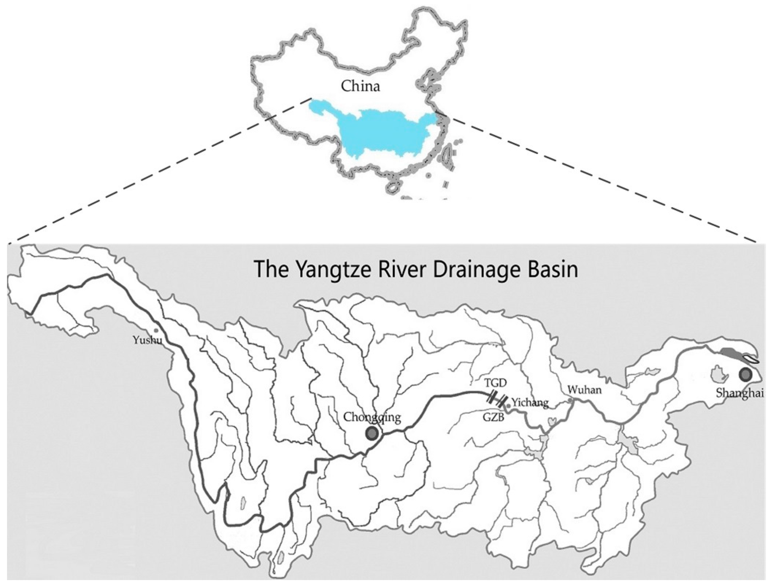
3.1. China’s Three Gorges Cascaded Hydropower System

The Yangtze River originates from the Qinghai–Tibet Plateau and flows eastward before debouching into the East China Sea near Shanghai. With a length of about 6300 km, the Yangtze River is China’s longest river and the world’s third longest river. The Yangtze River drains a wide basin of 1.8 million km², nearly one fifth of China’s territory and home to one third of China’s population. The stretches above Yichang form the upstream of the Yangtze River. The Yangtze River drops 120 m at the mountainous Three Gorges between Chongqing and Yichang. The TGD and GZB are located at the juncture of the upper and middle reaches of the Yangtze River. The TGD is 44 km upstream from Yichang, and the GZB is 38 km downstream from the TGD. Figure 1 shows the Yangtze River drainage basin and the TGD and GZB reservoirs. The TGD–GZB system plays a vitally important role in developing and harnessing the water resources of the Yangtze River as the system provides comprehensive benefits such as flood control, hydropower generation, navigation, sediment control, and water provisioning.

The middle and lower reaches of the Yangtze River is one of the most populous and developed areas in China, but is often hit by severe flooding. The essential reason for flooding is the river’s inadequate drainage capacity, compared with the huge volume of flood water. The TGD, with a huge flood control capacity of 22.15 billion m³ and by the tributary Jingjiang River as a flood relief channel, is able to effectively control the flooding from the upper reach.

China’s electricity supply has fallen short of demand in recent years because of the country’s rapid growing economy. Actually, the TGD is the world’s largest hydropower station in terms of installed hydropower generation capacity. The TGD is equipped with 32 units, with each unit having a capacity of 700 MW, totaling an installed capacity of 22,400 MW. The GZB has 21 units and its installed capacity is 2777 MW.

The river section between Chongqing and Yichang was full of dangerous reefs and shoals before the TGD was put into use. The section was only to be passed for fleets under 3000 tons. After the construction of the TGD, the back water reaches to Chongqing, and all the reefs/shoals were submerged and laid deep under water. The GZB is a run-of-the-river reservoir and reversely regulates the water releases from the TGD on a daily basis. Large ship locks were integrated with both the TGD and the GZB. As a result, 10,000-ton-class ships can sail all the way up to Chongqing from Shanghai.

The Yangtze River drainage basin is characterized by a subtropical climate initiated from the southeast Pacific Ocean and the Indian Ocean. The monsoon and precipitation cause seasonal variability in the river’s flow and the flood season is from June to September. Sediment discharge is uneven throughout the year and the quantity in May to October accounts for more than 90% of the annual sediment discharge. Hence, the TGD deals with sediment by lowering the reservoir water level to drain the floods with mud and sand during the flood season and by storing water during the drought season. To be specific, the TGD’s forebay elevation decreases to the flood control limit level (i.e., 145 m) during 1 June and 10 June; until 10 September, the TGD maintains its forebay elevation at 145 m in order to vacate enough storage for the incoming floods; then the TGD starts to impound water and the forebay elevation gradually increases to around 165 m at the end of September and to the normal pool level (i.e., 175 m) at the end of October or the beginning of November; from November to the next year’s May, the TGD gradually draws off water and is operated at high forebay elevations that are no less than the drought season control level (i.e., 155 m); the TGD’s forebay elevation should be no more than 155 m at the end of May. Figure 2 illustrates an example forebay elevation schedule of the TGD following the operation guidelines.

3.2. Problem Formulation

A generalized problem formulation for the single-objective operation of hydropower reservoir systems was introduced in [1]. The generalized problem formulation for the multi-objective operation is the same with that introduced in [1] except that the multi-objective operation involves multiple objectives.

The long-term planning of the TGD–GZB system is taken as the case for study in this paper. The planning horizon is a water year from 1 June to next year’s 31 May with 10-day time steps. For the TGD, its forebay elevation gradually decreases from 175 m in November to 155 m at the end of May, thus 16.5 billion m³ of water is released from the TGD to replenish water uses in the drought season. The present minimum outflow rate for the TGD in the drought season is 6000 m³/s. However, the middle and lower reaches of the Yangtze River actually require a higher outflow rate from the TGD–GZB system in order to facilitate navigation, satisfy agricultural, domestic and industrial water demands, withstand salt tide invasion near Shanghai, and sustain the riverine ecosystem. In addition, several large water diversion projects, including the eastern and central routes of the South-North Water Transfer Project as well as the Yangtze–Chao–Huai Project, have been built or are being built in the middle and lower reaches of the Yangtze River to divert water from the river to water scarce regions of China such as northern China and Anhui Province. In Spring 2011, the release of the TGD reached 12,000 m³/s for the purpose of alleviating severe drought downstream. In late February and early March 2014, the TGD’s outflow rate was increased to no less than 7000 m³/s to help combat serious salt tide invasion near Shanghai.

Two objectives are optimized simultaneously: one is to maximize the amount of hydropower generated from the TGD–GZB system over the planning horizon, and the other is to minimize the deviation from the outflow lower target so as to realize the system’s economic, environmental, and social benefits during the drought season. The maximizing-hydropower-generation objective f₁ is

$$\text{Max} f_1={\displaystyle \sum _{t=1}^{36}{\displaystyle \sum _{j=1}^2{P}_{j,t}\times {\Delta }_t}}$$

(1)

where t is the 10-day time step index; j is the reservoir index, with j = 1 and j = 2 respectively representing the TGD and the GZB; P_j,t is the power output of reservoir j in time step t; and Δ_t is the length of time step t. The minimizing-outflow-deviation objective f₂ is

$$\text{Min} f_2={\displaystyle \sum _{t=1}^{36}\max \{0,T-O_{2,t}\}\times {\Delta }_t}$$

(2)

where T is the preferred lower target value for the TGD–GZB system’s outflow rate and T > 6000 m³/s; and O_j,t is the outflow rate of reservoir j in time step t. Here the system’s outflow rate is the GZB’s outflow rate O_2,t. The two objectives conflict with each other. Operation of the system purely based on minimizing the outflow lower target deviation would lower the TGD’s water heads too rapidly in the drought season, thereby leading to the reduction of hydropower generation.

The problem essentially aims to schedule the power discharge and spillage rates of the two reservoirs in all the time steps over the planning horizon. The problem is subjected to the following physical and operational constraints.

(a) Outflow constraints.

$$0\le Q_{j,t}\le Q_{j,t}^{\max },j=1,2,t=1,2,\mathrm{...},36$$

(3)

$$0\le S_{j,t}\le S_j^{\max },j=1,2,t=1,2,\mathrm{...},36$$

(4)

$$O_{j,t}=Q_{j,t}+S_{j,t},j=1,2,t=1,2,\mathrm{...},36$$

(5)

$$O_{j,t}^{\min }\le O_{j,t}\le O_{j,t}^{\max },j=1,2,t=1,2,\mathrm{...},36$$

(6)

where Q_j,t is the power discharge rate of reservoir j in time step t; $Q_{j,t}^{\max }$ is the maximum power discharge rate of reservoir j in time step t; S_j,t is the spillage rate of reservoir j in time step t; $S_j^{\max }$ is the maximum spillage rate of reservoir j; O_j,t is the outflow rate of reservoir j in time step t; and $O_{j,t}^{\min }$ and $O_{j,t}^{\max }$ are respectively the minimum and maximum outflow rates of reservoir j in time step t. The TGD’s minimum outflow rate requirements are 10,000 m³/s during mid and late September, 8000 m³/s in October and 6000 m³/s in the drought season.

(b) Power output constraints.

$$P_{j,t}^{\min }\le P_{j,t}\le P_{j,t}^{\max },j=1,2,t=1,2,\mathrm{...},36$$

(7)

where $P_{j,t}^{\min }$ and $P_{j,t}^{\max }$ are respectively the minimum and maximum power outputs of reservoir j in time step t.

(c) Storage volume and forebay elevation constraints.

$$V_{j,1}=V_j^{\text{begin}},j=1,2$$

(8)

$$F_{j,t}^{\min }\le F_{j,t}\le F_{j,t}^{\max },j=1,2,t=2,3,\mathrm{...},37$$

(9)

$$F_{1,t+1}-F_{1,t}\le C_{\max },t=1,2,\mathrm{...},35$$

(10)

where V_j,t is the storage volume of reservoir j at the beginning of time step t; $V_j^{\text{begin}}$ is the initial storage volume limit of reservoir j; F_j,t is the forebay elevation of reservoir j at the beginning of time step t and it is a function of j’s geometry and storage volume; $F_{j,t}^{\min }$ and $F_{j,t}^{\max }$ are respectively the minimum and maximum forebay elevations of reservoir j at the beginning of time step t and when t = 37 they limit j’s final storage volume; and C_max is the variation limit of the TGD’s forebay elevations in consecutive time steps. For example, when the TGD’s forebay elevation gradually decreases from 175 m to 155 m in the drought season, the daily decrease is suggested to be no more than 0.6 m. The GZB’s forebay elevation is usually assumed to be fixed at the normal water level (i.e., 65 m) in the long-term planning.

(d) Water balance constraints.

$$V_{1,t+1}=V_{1,t}+I_{1,t}-O_{1,t}\times {\Delta }_t,t=1,2,\mathrm{...},36$$

(11)

$$V_{2,t+1}=V_{2,t}+I_{2,t}+O_{1,t}\times {\Delta }_t-O_{2,t}\times {\Delta }_t,t=1,2,\mathrm{...},36$$

(12)

where I_j,t is the natural inflow into reservoir j in time step t.

The power output P_j,t is a nonlinear function of the power discharge rate and water head, i.e.,

$$P_{j,t}=K_j\times Q_{j,t}\times H_{j,t}$$

(13)

where K_j is the synthetic power output coefficient of reservoir j; and H_j,t is the average water head of reservoir j in time step t. The amount of hydropower generated by reservoir j in time step t is thus given by P_j,t × Δ_t. The maximum power discharge rate $Q_{j,t}^{\max }$ and the maximum power output $P_{j,t}^{\max }$ both depend on H_j,t.

The water head H_j,t is calculated according to Equation (14).

$$H_{j,t}=\frac{F_{j,t}+F_{j,t+1}}{2}-R_{j,t}-H_{j,t}^{\text{loss}}$$

(14)

where R_j,t is the average tailrace elevation of reservoir j in time step t; and $H_{j,t}^{\text{loss}}$ is the average head loss of reservoir j in time step t. R_j,t is mainly dependent on j’s outflow rate. As the two reservoirs are close in distance, the upstream TGD’s tailrace elevation R_1,t is also affected by the downstream GZB’s forebay elevation F_2,t. The head loss is caused by friction.

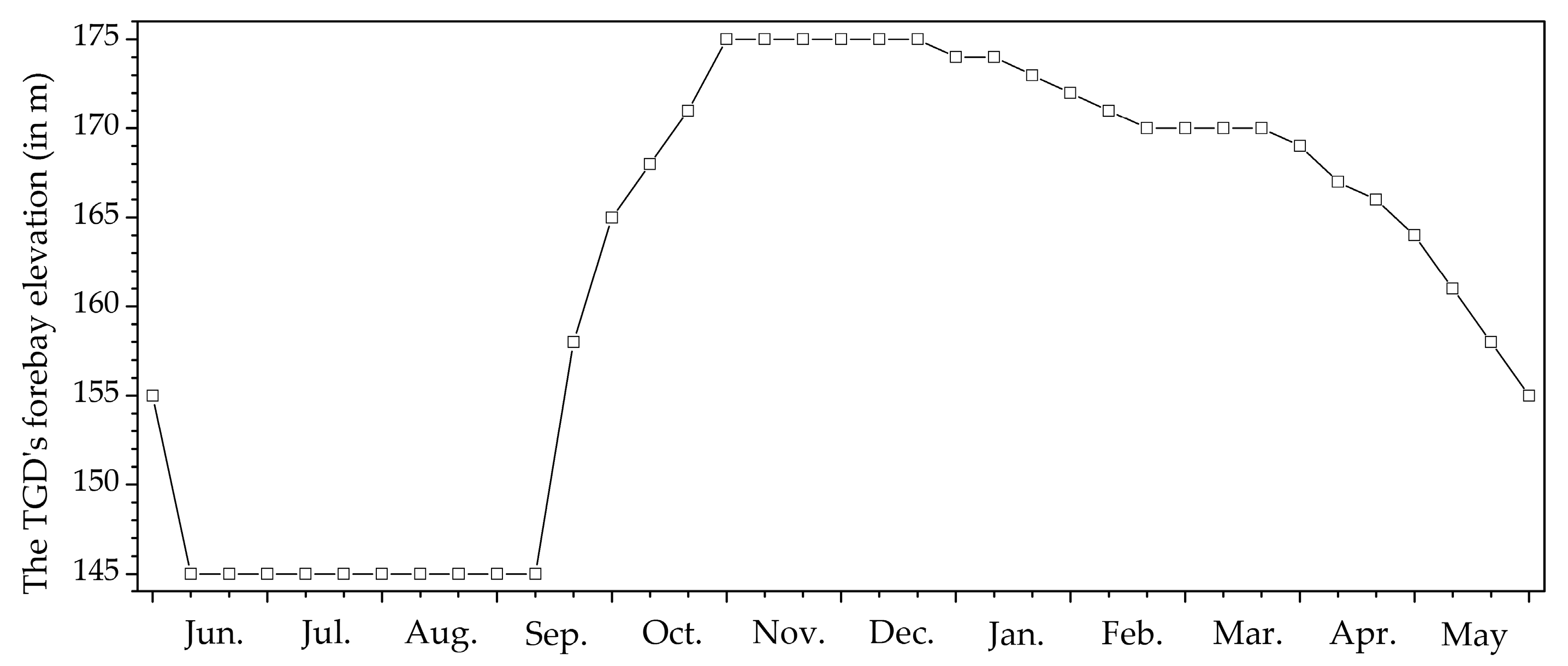
3.3. Determination of the Outflow Lower Target

Water management authorities worldwide have become increasingly aware of the environmental impacts and knock-on socio-economic implications of hydraulic projects. Indeed, impoundments (e.g., dams), diversion weirs, and/or exploitation of aquifers alter a stream and consequently affect the stream’s water quality, temperature, sediment movement and deposition, fish and wildlife, and associated human livelihoods and wellbeing. Environmental flow describes a flow regime required to accommodate human uses and sustain a healthy riverine ecosystem.

Recognition of the need to establish the extent to which the flow regime of a stream can be altered from natural has provided the impetus for research on environment flow assessment. The assessment methods are usually classified into four distinct categories, namely hydrological, hydraulic rating, habitat simulation, and holistic [17,18]. Hydrological methods rely primarily on the use of hydrological data, usually in the form of naturalized and historical flow records [17,18]. Hydraulic rating methods use changes in some simple hydraulic variable (e.g., wetted perimeter) usually measured across a river cross-section as a surrogate for habitat factors known or assuming to be limiting to biota [17,18]. Habitat simulation method assess environmental flow based on a detailed analysis of the quantity and suitability of physical habitat available to target species or assemblages under different discharges, using integrated hydrological, hydraulic and biological response data [17,18]. Holistic methods identify important flow events for some or all major components of a riverine ecosystem, and model relationships between flow and ecological, geomorphological and social responses, requiring considerable multi-disciplinary expertise and inputs [18]. Hydrological methods are rapid and non-resource-intensive, but they provide lower resolution results than the other three types of methods. Hence hydrological methods are considered to be most appropriate to be used at the planning level of water resources management when the flow estimates may be used as preliminary or interim management targets for the protection of native aquatic biodiversity and ecosystem integrity.

The Tennant method [19] is the most commonly applied hydrological environmental flow assessment method. The method links different percentages of the average annual flow (AAF) to different flow conditions, on a seasonal basis. The method was developed by Tennant in 1976 [19]. Tennant examined cross-section data from 11 streams in Montana, Nebraska and Wyoming in the United States. Tennant’s assessment of the environmental quality of different flow levels was based on the quantity of the physical habitat the flow level provided. At 10% of the AAF, he showed that water velocity and depth degraded and would only provide for lower limits for short-term survival of aquatic life. He considered that some higher percentage of the AAF would provide suitable water velocity and depth. The Tennant method indicates that 40% of the AAF is the outstanding flow level for the drought season, while 60% of the AAF is outstanding for the flood season. The optimum ranges for both seasons are 60%–100% of the AAF.

Long historical flow series during the period from year 1882 to 2002 were recorded at the Yichang hydrological station. The TGD was officially put into use in 2003. The AAF of the flow records is 14,260 m³/s. For the TGD–GZB cascaded hydropower system, the outflow lower target T is preliminarily set as 8556 m³/s which is 60% of the AAF and considered as the optimum environmental flow condition for both the flood season and the drought season according to the Tennant method. There are some important aquatic species such as the Chinese sturgeon and four major Chinese carps in the Yangtze River. Pan [20] showed that the appropriate environmental flow for the Chinese sturgeon during the spawning period between mid October and late November is at least 8000 m³/s, and that for the four major Chinese carps during the spawning period from late April to early July is also no less than 8000 m³/s. An outflow rate of 8556 m³/s for the TGD in the drought season could significantly increase annual navigation traffic capacity of the river reach between Yichang and Wuhan, decrease the navigation cost, satisfy agricultural, domestic and industrial water demands, and help withstand salt tide invasion near Shanghai.

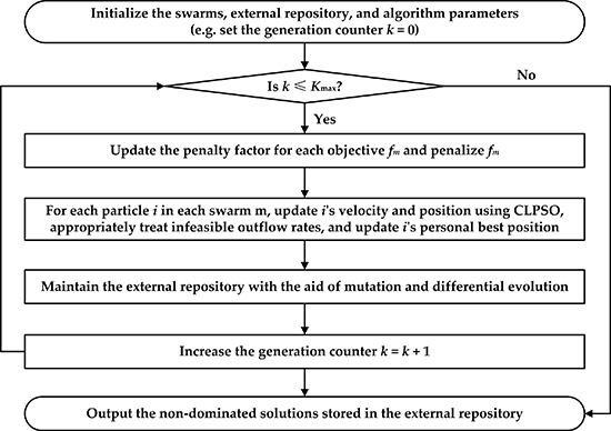
4. Optimization Framework Based on Multi-Swarm Comprehensive Learning Particle Swarm Optimization

4.1. Multi-Swarm Comprehensive Learning Particle Swarm Optimization

MSCLPSO [14] is a decomposition-based multi-swarm MOMH recently proposed by us. For a multi-objective optimization problem with M objectives f₁, f₂, …, and f_M, M swarms are used and each swarm m (1 ≤ m ≤ M) focuses on optimizing objective f_m using a state-of-the-art powerful single-objective PSO algorithm called comprehensive learning PSO (CLPSO) [21]. Elitists are stored into an external repository and the repository is shared by all the swarms.

Each swarm m does not learn from the elitists and the search experience of any other swarm. Let there be D decision variables, each particle i in swarm m is associated with a D-dimensional position Pos_m,i = (Pos_m,i,1, Pos_m,i,2, …, Pos_m,i,D) and a D-dimensional velocity Vel_m,i = (Vel_m,i,1, Vel_m,i,2, …, Vel_m,i,D). In each generation, Vel_m,i and Pos_m,i are updated as follows.

$$Ve{l}_{m,i,d}=w\times Ve{l}_{m,i,d}+c\times r_{m,i,d}\times (Ex{e}_{m,i,d}-Po{s}_{m,i,d})$$

(15)

$$Po{s}_{m,i,d}=Po{s}_{m,i,d}+Ve{l}_{m,i,d}$$

(16)

where d (1 ≤ d ≤ D) is the dimension index; w is the inertia weight and is suggested to linearly decrease from 0.9 to 0.4 [21]; c is the acceleration coefficient and c is suggested to be 1.5 [21]; r_m,i,d is a random number uniformly distributed in [0, 1]; and Exe_m,i = (Exe_m,i,1, Exe_m,i,2, …, Exe_m,i,D) is the guidance vector of exemplars. Exe_m,i,d is dimension d of particle i’s personal best position Pbest_m,i or that of some other particle selected within swarm m using a tournament procedure. The personal best position Pbest_m,i = (Pbest_m,i,1, Pbest_m,i,2, …, Pbest_m,i,D) is the historical best position of i.

The external repository (denoted as Rep) is initialized to be empty. As the number of elitists quickly grows during the run, Rep has a fixed maximum size L_max. Rep is maintained as follows in every generation: (1) A temporary set Tmp is initialized to be empty; (2) copy all the elitists in Rep to Tmp; (3) copy each particle’s current position to Tmp; (4) apply mutation to some elitists randomly selected from Rep on a randomly selected dimension and add the mutated elitists to Tmp; (5) apply DE to a number of extreme and least crowded elitists in Rep on every dimension and add the differentially evolved elitists to Tmp; (6) remove any dominated individual from the solutions in Tmp; (7) sort the non-dominated solutions in Tmp using respectively the crowding distance technique [8] for 2-objective problems and the M-nearest-neighbors product-based vicinity distance technique [22] for problems with more than two objectives; (8) if the number of non-dominated solutions in Tmp is larger than L_max, let the first L_max solutions to stay in Tmp and remove the other solutions from Tmp; and (9) remove all the elitists in Rep and copy all the non-dominated solutions in Tmp to Rep. In Step (8), letting the non-dominated solutions with larger crowding/vicinity distances to stay helps to preserve the diversity of the resulting non-dominated solutions on the Pareto front.

Non-dominated solutions and the Pareto front are defined in the objective space. A Pareto-optimal decision vector is the D-dimensional vector of decision variables of a non-dominated solution. The Pareto set is the set of all the Pareto-optimal decision vectors. Actually, the personal best positions and the elitists carry useful information about the Pareto set. The mutation strategy adopted in MSCLPSO exploits the personal best positions and the differences of the elitists. After a sufficient number of generations, the personal best position Pbest_m,i of each particle i in each swarm m is an exact-optimum or near-optimum corresponding to objective f_m. If the Pareto-optimal decision vectors are indifferent on dimension d, as Pbest_m,i,d is close to dimension d of the Pareto-optimal decision vector that is optimal on objective f_m, learning from Pbest_m,i,d contributes to the search of the Pareto set on dimension d; on the other hand, if the Pareto set is complicated on dimension d, the personal best positions obtained by different swarms often differ considerably on that dimension, accordingly learning from Pbest_m,i,d leads to the search of different regions of the Pareto set on dimension d. In addition, the dimensional difference of two different elitists selected from the external repository Rep is often small and could be large respectively in the simple and complicated cases with respect to the Pareto set on dimension d, thereby learning from the differences of the elitists also benefit the search of the Pareto set.

DE helps to evolve an elitist on every dimension. An elitist that is extreme on a single objective may actually be crowded, however it may be still far from the corresponding true extreme non-dominated solution on the Pareto front. The application of DE to the extreme and least crowded elitists is expected to improve the diversity of the elitists.

4.2. Application Implementation of Multi-Swarm Comprehensive Learning Particle Swarm Optimization

In [1], we have addressed the single-objective operation of multi-reservoir hydropower systems using an optimizer called enhanced CLPSO [23]. Here for the multi-objective application implementation of MSCLPSO, each particle i’s position Pos_m,i is a vector representing candidate outflow rates of all the reservoirs in all the time steps [1]. The power discharge rate Q_i,t and spillage rate S_i,t can be conveniently determined from the outflow rate O_i,t [1]. Infeasible outflow rates are appropriately treated, the constrained problem is converted to an unconstrained one through penalizing the constraints, and the penalty factor is dynamically adjusted using the strategies introduced in [1]. The penalty factor parameters (i.e., minimum penalty factor ${\mathsf{\lambda }}_m^{\min }$ and maximum penalty factor ${\mathsf{\lambda }}_m^{\max }$) could be different for each objective f_m. The optimization framework is summarized in Figure 3, where K_max is the pre-specified maximum number of generations.

5. Experimental Studies

5.1. Co-Evolutionary Multi-Swarm Particle Swarm Optimization

CMPSO [15] is the same with MSCLPSO in terms of using multiple swarms. CMPSO differs from MSCLPSO in the way to update the particles and the way to evolve the elitists.

In CMPSO, the dimensional velocity Vel_m,i of each particle i in swarm m is updated on each dimension d according to Equation (17).

$$\begin{array}{l}Ve{l}_{m,i,d}=w\times Ve{l}_{m,i,d}+c_1\times r_{1,d}\times (Pbes{t}_{m,i,d}-Po{s}_{m,i,d})+\\ c_2\times r_{2,d}\times (Gbes{t}_{m,d}-Po{s}_{m,i,d})+c_3\times r_{3,d}\times (Y_{l,d}-Po{s}_{m,i,d})\end{array}$$

(17)

where Gbest_m = (Gbest_m,1, Gbest_m,2, …, Gbest_m,D) is the historical best position (i.e., global best position) out of all the particles in swarm m; l is an elitist randomly selected from the external repository Rep; Y_l = (Y_l,1, Y_l,2, …, Y_l,D) is the decision vector of elitist l; $c_1=c_2=c_3=4/3$; and r_1,d, r_2,d and r_3,d are random numbers uniformly distributed in [0, 1]. As we can see, CMPSO updates each particle i’s flight trajectory based on not only i’s host swarm’s search experience but also indirectly the other swarms’ search experience. In contrast, MSCLPSO updates each particle i’s velocity purely based on the search experience of the particles in i’s host swarm because information determined based on Pareto dominance or some other single objective might not contribute to the optimization on i’s associated objective.

CMPSO involves no DE. In each generation, CMPSO maintains the external repository through applying Gaussian mutation to each of the elitists. To be specific, for each elitist l in the external repository Rep, l’s decision vector Y_l is copied as Z_l = (Z_l,1, Z_l,2, …, Z_l,D). A dimension d is randomly selected. Let r_gmut be a random number generated from a standard normal distribution, Z_l,d is mutated according to Equation (18).

$$Z_{l,d}=Z_{l,d}+r_{\text{gmut}}\times (Po{s}_d^{\max }-Po{s}_d^{\min })$$

(18)

where $[Po{s}_d^{\min },Po{s}_d^{\max }]$ is the range of the search space on dimension d. It can be seen that the mutation strategy of CMPSO does not exploit the personal best positions nor the elitists. CMPSO puts the personal best positions, elitists and mutated individuals into a temporary set and selects non-dominated solutions from the temporary set into the external repository. CMPSO uses the crowding distance technique [8] to preserve the diversity of the elitists.

5.2. Performance Metrics

As the true Pareto front is unknown for the case study of the TGD–GZB cascaded hydropower system, metrics such as the inverted generational distance [8,14,15] cannot be used because the calculation of the metrics depends on the true Pareto front. Instead, the following performance metrics are used to evaluate the performance of MSCLPSO and CMPSO on the case study.

(1) The set coverage metric [24]. The resulting set of non-dominated solutions from a single run of MSCLPSO and that from a single run of CMPSO are processed to yield two numbers: the percentage of the non-dominated solutions obtained from CMPSO which are weakly dominated by (i.e., equal to or dominated by) the resulting solutions of MSCLPSO, and vice versa. Let the set of non-dominated solutions obtained from MSCLPSO be Rep_ms and that from CMPSO be Rep_cm, two values SC(MSCLPSO, CMPSO) and SC(CMPSO, MSCLPSO) are calculated respectively according to Equations (19) and (20).

$$SC(\text{MSCLPSO},\text{CMPSO})=\frac{\left|\{l_{\text{cm}}\in Re{p}_{\text{cm}}|\exists l_{\text{ms}}\in Re{p}_{\text{ms}},l_{\text{ms}}\text{weakly dominates} l_{\text{cm}}\}\right|}{\left|Re{p}_{\text{cm}}\right|}$$

(19)

The metric value lies in [0, 1]. SC(MSCLPSO, CMPSO) = 1 means that all the solutions in Rep_cm are weakly dominated by those of Rep_ms, while SC(MSCLPSO, CMPSO) = 0 represents the situation when none of the solutions in Rep_cm are weakly dominated by those of Rep_ms.

$$SC(\text{CMLPSO},\text{MSCLPSO})=\frac{\left|\{l_{\text{ms}}\in Re{p}_{\text{ms}}|\exists l_{\text{cm}}\in Re{p}_{\text{cm}},l_{\text{cm}}\text{weakly dominates} l_{\text{ms}}\}\right|}{\left|Re{p}_{\text{ms}}\right|}$$

(20)

Since the domination operator is not symmetric, i.e., SC(MSCLPSO, CMPSO) is not necessarily equal to 1 – SC(CMPSO, MSCLPSO), it thus requires to calculate both values to understand how many solutions of Rep_cm are weakly dominated by Rep_ms and vice versa.

(2) The spacing metric [25]. This metric aims at assessing the spread of the non-dominated solutions. It is calculated as follows.

$$SP=\sqrt{\frac{{\displaystyle \sum _{l=1}^L{(O{d}_l-O{d}_{\text{mean}})}^2}}{L-1}}$$

(21)

where L is the number of elitists in the external repository Rep; Od_l is a distance measure related to each elitist l; and Od_mean is the mean value of the distance measure (i.e., $O{d}_{\text{mean}}={\displaystyle {\sum }_{l=1}^{L}O{d}_l}/L$). In [25], Od_l is the degree one distance between l and l’s closest neighbor; this approach might make a wrong judgment for the spread of the non-dominated solutions, e.g., if l is close to one elitist but far from all the other elitists. Therefore, we propose to calculate Od_l based on a modification of the crowding distance concept introduced in [8]. The calculation of Od_l follows two steps.

Step (1) For each objective f_m, sort the elitists in Rep in the increasing order of their fitness values on f_m if f_m is a minimization objective or in the decreasing order if f_m is a maximization objective. Calculate the objective-related distance measure of each elitist l according to Equation (22).

$$O{d}_{l,m}=\frac{1}{f_m(Y_L)-f_m(Y_1)}\times \{\begin{array}{l}(f_m(Y_2)-f_m(Y_1)), \text{if} l =1\\ (f_m(Y_L)-f_m(Y_{L-1})), \text{else if} l = L\\ (f_m(Y_{l+1})-f_m(Y_{l-1})), \text{otherwise}\end{array}$$

(22)

Step (2) Calculate Od_l according to Equation (23).

$$O{d}_l={\displaystyle \sum _{m=1}^{2}O{d}_{l,m}}$$

(23)

The calculation of Od_l,m differs from that in [8] in that the two extreme elitists 1 and L are assigned finite distance values here. The desired value for the spacing metric is zero, which means that the non-dominated solutions are equidistantly spaced.

(3) The optimal value of the resulting non-dominated solutions on each single objective. For each objective f_m, the optimal value OP_m of the resulting non-dominated solution on f_m is determined according to Equation (24).

$$O{P}_m=\{\begin{array}{l}\min \{f_m(Y_l),\forall l\in Rep\}, \text{if} f_m \text{is a minmizaion objective}\\ \max \{f_m(Y_l),\forall l\in Rep\}, \text{otherwise}\end{array}$$

(24)

OP_m helps to assess whether the algorithm can find the extreme value on objective f_m.

(4) The sum of the violation costs of the resulting non-dominated solutions VC, which is calculated according to Equation (25).

$$VC={\displaystyle \sum _{l=1}^{L}Vio(Y_l)}$$

(25)

where Vio(Y_l) is the violation cost of elitist l with respect to the constraints as expressed in Equations (3) to (12) and is calculated as in the manner introduced in [1]. VC = 0 means that all the resulting non-dominated solutions are feasible.

(5) The execution time of each algorithm.

5.3. Algorithm Parameters

Unless otherwise specified, the algorithm parameters of MSCLPSO and CMPSO respectively take the recommended values specified in [14,15]. The number of particles in each swarm is set as 20. For both algorithms, the dimensional velocity Vel_m,i,d is clamped to a positive value $Ve{l}_d^{\max }$. If $Ve{l}_{m,i,d}>Ve{l}_d^{\max }$, then Vel_m,i,d is set to $Ve{l}_d^{\max }$; or if $Ve{l}_{m,i,d}<-Ve{l}_d^{\max }$, then Vel_m,i,d is set to $-Ve{l}_d^{\max }$. Here $Ve{l}_d^{\max }=0.06\times (Po{s}_d^{\max }-Po{s}_d^{\min })$. For objective f₁, the minimum penalty factor ${\mathsf{\lambda }}_1^{\min }=2.75\times {10}^9$ and the maximum penalty factor ${\mathsf{\lambda }}_1^{\max }={\mathsf{\lambda }}_1^{\min }\times {10}^{14}$. For objective f₂, ${\mathsf{\lambda }}_2^{\min }=4.95\times {10}^8$ and ${\mathsf{\lambda }}_2^{\max }={\mathsf{\lambda }}_2^{\min }\times {10}^{14}$. ε-dominance [26] is used and ε = 10,000. The maximum number of elitists L_max = 100. MSCLPSO and CMPSO are executed for 30 runs, with each run lasting for 10,000 generations. The inflow series in the normal water year 2005–2006 are taken as the hydrological inputs

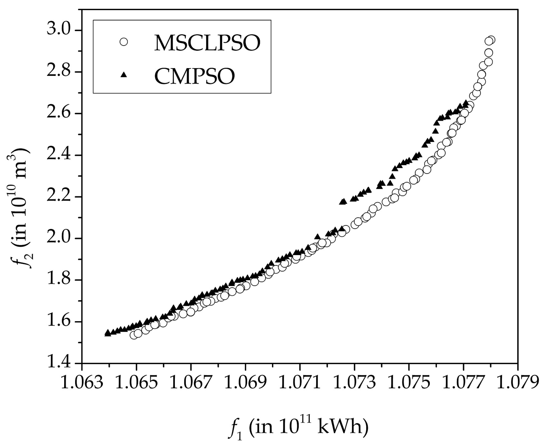
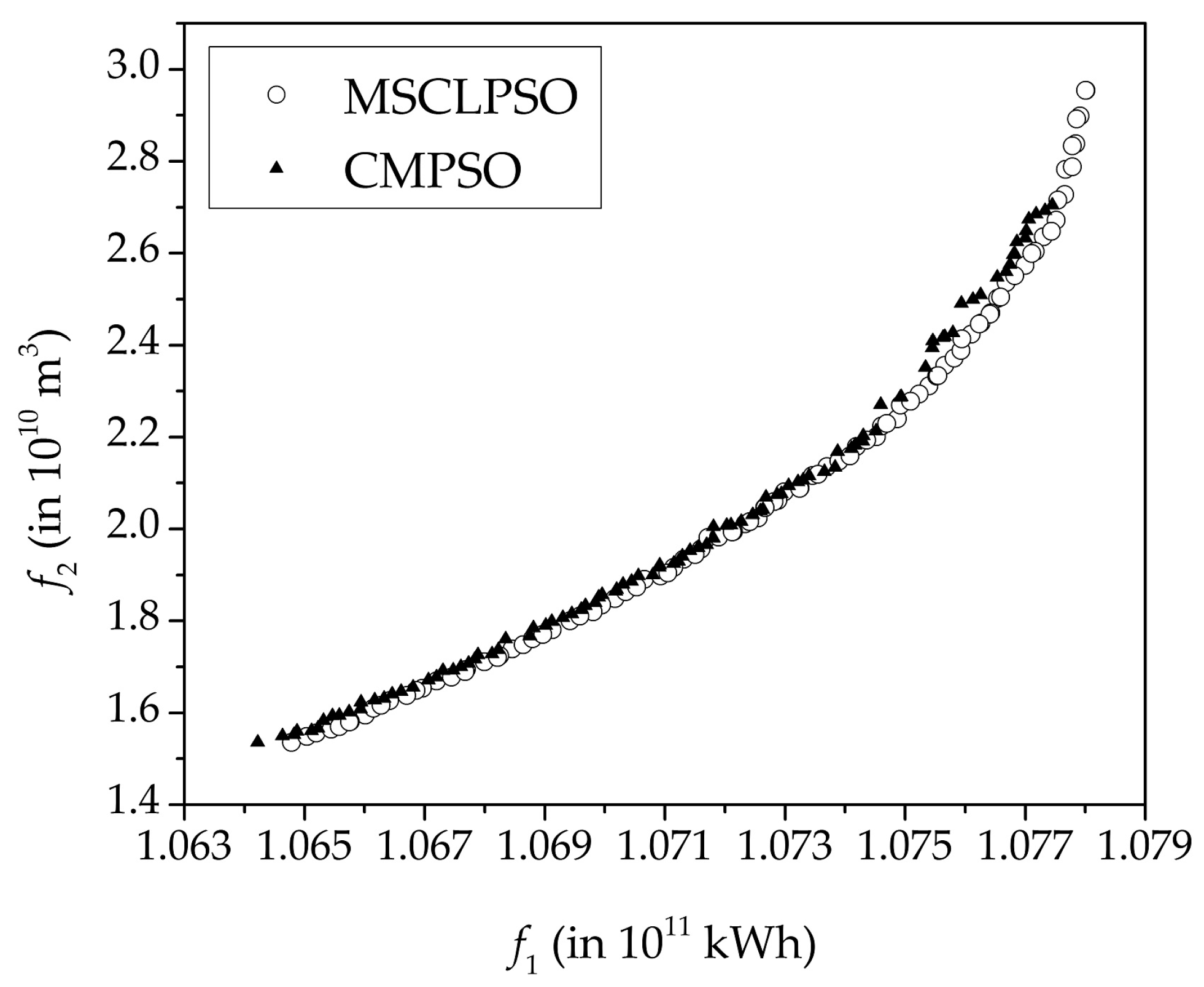
5.4. Experimental Results

The set coverage metric results are listed in

Table 1. The set coverage metric results.

SC(MSCLPSO, CMPSO)				SC(CMPSO, MSCLPSO)
Mean	SD	Best	Worst	Mean	SD	Best	Worst
0.88	9.30 × 10−2	0.99	0.66	0.02	2.12 × 10−2	0	0.08

.

Table 2. The spacing metric results.

MSCLPSO				CMPSO
Mean	SD	Best	Worst	Mean	SD	Best	Worst
spacing metric result				spacing metric result
1.19 × 10−2	1.01 × 10−3	9.72 × 10−3	1.37 × 10−2	2.70 × 10−2	6.12 × 10−3	1.76 × 10−2	3.98 × 10−2

lists the spacing metric results. In Table 1 and Table 2, “SD” refers to standard deviation. The OP_m, VC, and execution time results are given

Table 3. The OP_m, VC and execution time results.

Performance Metric		MSCLPSO		CMPSO
		Objective 1	Objective 2	Objective 1	Objective 2
OPm	Mean	1.0780 × 1011 kWh	1.5361 × 1010 m3	1.0775 × 1011 kWh	1.5361 × 1010 m3
	Best	1.0780 × 1011 kWh	1.5361 × 1010 m3	1.0779 × 1011 kWh	1.5361 × 1010 m3
	Worst	1.0780 × 1011 kWh	1.5361 × 1010 m3	1.0756 × 1011 kWh	1.5361 × 1010 m3
Average VC		0		0
Average execution time (in s)		7.03		13.13

.

Table 4. Best final single-objective results obtained by the swarms.

Best Final Single-Objective Result		MSCLPSO		CMPSO
		Swarm 1	Swarm 2	Swarm 1	Swarm 2
Fitness	Mean	1.0780 × 1011 kWh	1.5361 × 1010 m3	1.0752 × 1011 kWh	1.5361 × 1010 m3
	Best	1.0780 × 1011 kWh	1.5361 × 1010 m3	1.0766 × 1011 kWh	1.5361 × 1010 m3
	Worst	1.0780 × 1011 kWh	1.5361 × 1010 m3	1.0726 × 1011 kWh	1.5361 × 1010 m3
Average violation cost		0	0	4.81 × 10−17	0

lists the best final single-objective results obtained by the swarms of the two MOMHs. Figure 4 shows the non-dominated solutions obtained by MSCLPSO and CMPSO when SC(MSCLPSO, CMPSO) = 0.99 and SC(CMPSO, MSCLPSO) = 0, while Figure 5 illustrates those obtained by the two MOMHs in the best runs in terms of the spacing metric.

Comparison of the set coverage metric results: As can be observed from the set coverage metric results given in Table 1, the mean and best SC(MSCLPSO, CMPSO) results are close to 1, whereas the mean and worst SC(CMPSO, MSCLPSO) results are close to 0. The observations indicate that in all of the runs, most of the solutions obtained from CMPSO are weakly dominated by those from MSCLPSO, whereas none or only a few of the solutions obtained from MSCLPSO are weakly dominated by those from CMPSO. Accordingly, the non-dominated solutions resulted from MSCLPSO converge better than those resulted from CMPSO. The two Pareto fronts illustrated in Figure 4 also verify that MSCLPSO is superior to CMPSO in terms of convergence.

Comparison of the spacing metric results: As the spacing metric results given in Table 2 show, the mean, best and worst spacing metric results of MSCLPSO are significantly better than those of CMPSO. The best and worst spacing metric results of MSCLPSO are close to the mean result. As we can see from Figure 4 and Figure 5, the final non-dominated solutions obtained from MSCLPSO exhibit good spread over the Pareto front; in contrast, the solutions obtained by CMPSO are not uniformly distributed. All the observations demonstrate that MSCLPSO can robustly find non-dominated solutions spread reasonably over the Pareto front and MSCLPSO beats CMPSO in terms of diversity.

The extreme solution: It can be observed from the OP_m results given in Table 3 that MSCLPSO can find the extreme solution on each objective in the final set of non-dominated solutions whereas CMPSO fails on the maximizing-hydropower-generation objective, in each run. Table 4 shows the same phenomenon for the single-objective results obtained by the swarms of the two MOMHs.

The feasibility of the non-dominated solutions: A can be seen from the VC results given in Table 3, the average VC results of MSCLPSO and CMPSO are both zero, meaning that all the resulting non-dominated solutions are feasible in each run.

The execution time: Both MOMHs execute for 10,000 generations in each run. Actually, CMPSO consumes more function evaluations than MSCLPSO with the same number of generations because CMPSO applies mutation to each of the stored elitists whereas MSCLPSO applies mutation and DE to just some of the elitists. Accordingly, CMPSO takes significantly more execution time in each run than MSCLPSO, as the average execution time results in Table 3 shows.

Analysis of the results: Although CMPSO takes more function evaluations than MSCLPSO, CMPSO is significantly worse than MSCLPSO in terms of the performance concerns such as convergence, diversity, and the ability to find extreme solutions. The satisfactory performance of MSCLPSO owes to the following two factors: (1) in MSCLPSO, each swarm focuses on optimizing the associated single objective strictly using CLPSO, without learning from the elitists or any other swarm; and (2) as the personal best positions and the elitists carry useful information about the Pareto set, the mutation and DE strategies adopted in MSCLPSO help discover the true Pareto front. The particle learning mechanism as expressed in Equation (17) might hinder CMPSO from finding extreme solutions because the Y_l term in Equation (17) might not benefit the optimization on objective f_m.

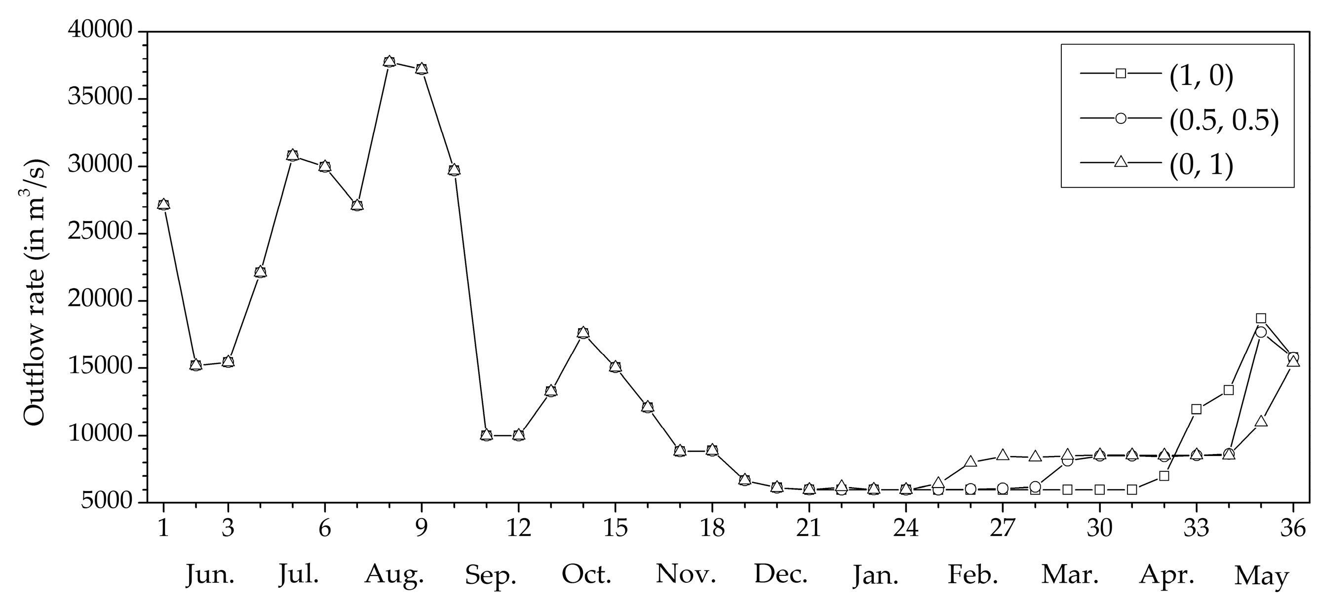
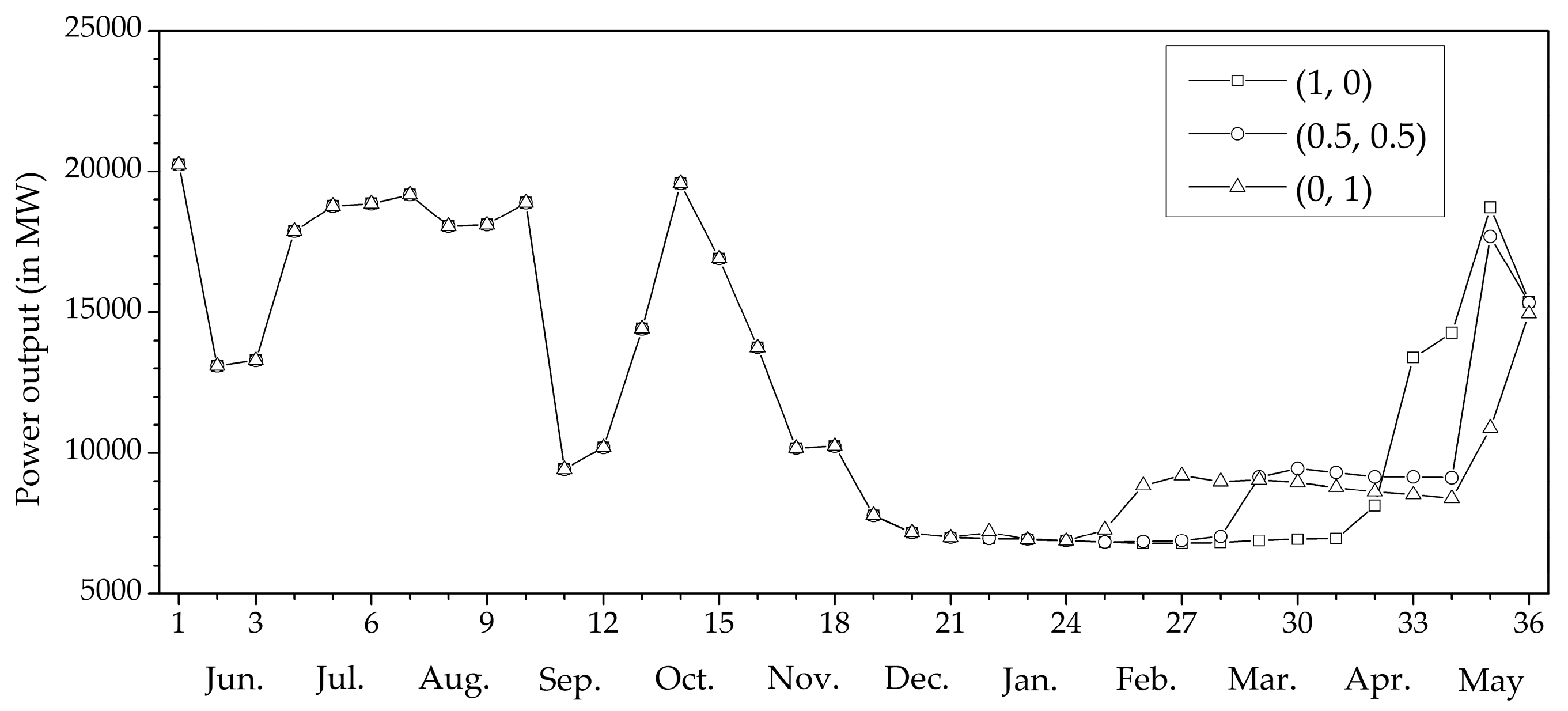
5.5. The Final Tradeoff

The final tradeoff is determined from the 100 non-dominated solutions obtained from MSCLPSO in the best run in terms of the spacing metric using the technique for order of preference by similarity to ideal solution (TOPSIS) [27]. TOPSIS is a commonly used multi-criteria decision analysis (MCDA) [28] method. MCDA involves multiple alternatives evaluated on multiple criteria. The weights of the criteria need to be determined in order to indicate the relative importance of the criteria. The weights can be determined subjectively, objectively, or in a manner combing the strengths of subjective and objective approaches [29]. In TOPSIS, two artificial alternatives are hypothesized, i.e., the ideal alternative which is the alternative having the best levels for all the criteria considered and the negative ideal alternative which is the alternative having the worst criteria values. TOPSIS selects the alternative that is closest to the ideal alternative and farthest from the negative ideal alternative as the final tradeoff.

We look at three tradeoffs corresponding to the (1, 0), (0.5, 0.5,) and (0, 1) weight combinations selected by the TOPSIS approach. The objective values of the three tradeoffs are listed in

Table 5. Example final tradeoffs.

Weight		Tradeoff
Objective 1	Objective 2	Objective 1	Objective 2
1	0	1.0780 × 1011 kWh	2.9545 × 1010 m3
0.5	0.5	1.0741 × 1011 kWh	2.1589 × 1010 m3
0	1	1.0648 × 1011 kWh	1.5361 × 1010 m3

. Figure 6 and Figure 7 respectively depict the TGD–GZB system’s outflow rates and power outputs of the three tradeoffs. As can be observed from Figure 6 and Figure 7, the three tradeoffs differ in the outflow rates only for the period from February to May. The (1, 0)-tradeoff keeps the outflow rates around the lower bound (i.e., 6000 m³/s) in February, March and early April. The (0.5, 0.5)-tradeoff starts increasing the outflow rate in March, while the (0, 1)-tradeoff starts increasing in February. Hydropower generation is dependent on both power discharge rate and water head. The (0.5, 0.5)-tradeoff and (0, 1)-tradeoff discharge more water than the (1, 0)-tradeoff between February and mid April, hence leading to more hydropower generation in that period. However, for the (0.5, 0.5)-tradeoff and (0, 1)-tradeoff, less storage is left after mid April and hence the two tradeoffs discharge significantly less water than the (1, 0)-tradeoff between late April and mid May. As a result, the (1, 0)-tradeoff still generates the largest amount of electricity over the planning horizon.

6. Conclusions

An optimization framework based on MSCLPSO has been proposed in this paper to address the multi-objective operation of hydropower reservoir systems. MSCLPSO uses multiple swarms, with each swarm focusing on optimizing a separate objective. Elitists are stored in an external repository and the repository is shared by all the swarms. The personal best positions and the elitists carry useful information about the Pareto set. Through exploiting such useful information, MSCLPSO adopts mutation and DE to evolve the elitists and tries to discover the true Pareto front. The physical and operational constraints are appropriately handled. The long-term sustainable planning of China’s TGD–GZB cascaded hydropower system has been taken as the case for study. Two conflicting objectives, i.e., maximizing hydropower generation and minimizing deviation from the outflow lower target to realize the system’s economic, environmental and social benefits during the drought season, are optimized simultaneously. The outflow lower target is determined by taking into account various concerns for the sustainable development of the TGD–GZB system. Experimental results have demonstrated that the optimization framework helps to robustly derive multiple feasible solutions distributed reasonably over the Pareto front in one single run and significantly outperforms CMPSO in terms of convergence, diversity and extremity of the resulting non-dominated solutions.

In the future, the performance of MSCLPSO is to be further enhanced. We will investigate designing adaptive search strategies to improve the algorithm’s efficiency on various types of problems. In addition, more cases related to the multi-objective operation of hydropower reservoir systems will be studied. For example, it is beneficial to understand how the operation can simultaneously maximize hydropower generation and minimize the negative impact caused by extreme floods and droughts with the occurrence of climate change. For another example, the short-term multi-objective operation of the TGD–GZB system with 10-day planning horizon and daily time steps will be studied. The long-term optimization results can be fed into the short-term optimization as constraints. Operation rules can be extracted from the results optimized over an ensemble of historical or synthetically generated inflows using a regression (e.g., auto-regressive moving average) or artificial intelligence (e.g., genetic programming) method to guide the operation of the TGD–GZB system in practice.

References

1. Zhang, X.; Yu, X.; Qin, H. Optimal operation of multi-reservoir hydropower systems using enhanced comprehensive learning particle swarm optimization. J. Hydro-Environ. Res. 2016, 10, 50–63. [Google Scholar] [CrossRef]
2. Chen, L.; McPhee, J.; Yeh, W.W. A diversified multiobjective GA for optimizing reservoir rule curves. Adv. Water Resour. 2007, 30, 1082–1093. [Google Scholar] [CrossRef]
3. Reddy, M.J.; Kumar, D.N. Multi-objective particle swarm optimization for generating optimal trade-offs in reservoir operation. Hydrol. Processes 2007, 21, 2897–2909. [Google Scholar] [CrossRef]
4. Zhang, H.; Zhou, J.; Fang, N.; Zhang, R.; Zhang, Y. An efficient multi-objective adaptive differential evolution with chaotic neuron network and its application on long-term hydropower operation with considering ecological environment problem. Int. J. Electr. Power Energy Syst. 2013, 45, 60–70. [Google Scholar] [CrossRef]
5. Liu, X.; Guo, S.; Liu, P.; Chen, L.; Li, X. Deriving optimal refill rules for multi-purpose reservoir operation. Water Resour. Manag. 2011, 25, 431–448. [Google Scholar] [CrossRef]
6. Yang, T.; Gao, X.; Sellars, S.; Sorooshian, S. Improving the multiobjective evolutionary optimization algorithm for hydropower reservoir operations in the California Oroville-Thermalito complex. Environ. Model. Softw. 2015, 69, 262–279. [Google Scholar] [CrossRef]
7. Zhang, R.; Zhou, J.; Wang, Y. Multi-objective optimization of hydrothermal energy system considering economic and environmental aspects. Int. J. Electr. Power Energy Syst. 2012, 42, 384–395. [Google Scholar] [CrossRef]
8. Deb, K.; Pratap, A.; Agarwal, S.K.; Meyarivan, T. A fast and elitist multiobjective genetic algorithm: NSGA-II. IEEE Trans. Evolut. Comput. 2002, 6, 182–197. [Google Scholar] [CrossRef]
9. Cohon, J.L.; Marks, D.H. A review and evaluation of multiobjective programming techniques. Water Resour. Res. 1975, 11, 208–220. [Google Scholar] [CrossRef]
10. Miettinen, K. Nonlinear Multiobjective Optimization; Kluwer Academic Publishers: Boston, MA, USA, 1999. [Google Scholar]
11. Schardong, A.; Simonovic, S.P.; Vasan, A. Multiobjective evolutionary approach to optimal reservoir operation. J. Comput. Civil Eng. 2012, 27, 139–147. [Google Scholar] [CrossRef]
12. Qin, H.; Zhou, J.; Lu, Y.; Li, Y.; Zhang, Y. Multi-objective cultured differential evolution for generating optimal trade-offs in reservoir flood control operation. Water Resour. Manag. 2010, 24, 2611–2632. [Google Scholar] [CrossRef]
13. Li, Y.; Zhou, J.; Zhang, Y.; Qin, H.; Liu, L. Novel multiobjective shuffled frog leaping algorithm with application to reservoir flood control operation. J. Water Resour. Plan. Manag. 2010, 136, 217–226. [Google Scholar] [CrossRef]
14. Yu, X.; Zhang, X. Multiswarm comprehensive learning particle swarm optimization for solving multiobjective optimization problems. Swarm Evolut. Comput. 2016. submitted. [Google Scholar]
15. Zhan, Z.; Li, J.; Cao, J.; Zhang, J.; Chung, H.S.; Shi, Y. Multiple populations for multiple objectives: A coevolutionary technique for solving multiobjective optimization problems. IEEE Trans. Cybern. 2013, 43, 445–463. [Google Scholar] [CrossRef] [PubMed]
16. Zhang, Q.; Li, H. MOEA/D: A multiobjective evolutionary algorithm based on decomposition. IEEE Trans. Evolut. Comput. 2007, 11, 712–731. [Google Scholar] [CrossRef]
17. Jowett, I.G. Instream flow methods: A comparison of approaches. Regul. Rivers Res. Manag. 1997, 13, 115–127. [Google Scholar] [CrossRef]
18. Tharme, R.E. A global perspective on environmental flow assessment: Emerging trends in the development and application of environmental flow methodologies for rivers. River Res. Appl. 2003, 19, 397–441. [Google Scholar] [CrossRef]
19. Tennant, D.L. Instream flow regimens for fish, wildlife, recreation and related environmental resources. Fisheries 1976, 1, 6–10. [Google Scholar] [CrossRef]
20. Pan, M. Research on Ecological Operation Objectives of Three Gorges Reservoir. Master’s Thesis, Donghua University, Shanghai, China, 2011. [Google Scholar]
21. Liang, J.J.; Qin, A.K.; Suganthan, P.N.; Baskar, S. Comprehensive learning particle swarm optimizer for global optimization of multimodal functions. IEEE Trans. Evolut. Comput. 2006, 10, 281–295. [Google Scholar] [CrossRef]
22. Kukkonen, S.; Deb, K. A fast and effective method for pruning of non-dominated solutions in many-objective problems. In Proceedings of the 9th International Conference on Parallel Problem Solving from Nature, Reykjavik, Iceland, 9–13 September 2006; pp. 553–562.
23. Yu, X.; Zhang, X. Enhanced comprehensive learning particle swarm optimization. Appl. Math. Comput. 2014, 242, 265–276. [Google Scholar] [CrossRef]
24. Zitzler, E.; Thiele, L. Multiobjective evolutionary algorithms: A comparative case study and the strength Pareto approach. IEEE Trans. Evolut. Comput. 1999, 3, 257–271. [Google Scholar] [CrossRef]
25. Schott, J.R. Fault Tolerant Design Using Single and Multicriteria Genetic Algorithm Optimization. Master’s Thesis, Massachusetts Institute of Technology, Cambridge, MA, USA, 1995. [Google Scholar]
26. Laumanns, M.; Thiele, L.; Deb, K.; Zitzler, E. Combining convergence and diversity in evolutionary multiobjective optimization. Evolut. Comput. 2002, 10, 263–282. [Google Scholar] [CrossRef] [PubMed]
27. Hwang, C.L.; Yoon, K. Multiple Attribute Decision Making: Methods and Applications; Springer-Verlag: Berlin, Germany, 1981. [Google Scholar]
28. Wang, J.; Jing, Y.; Zhang, C.; Zhao, J. Review on multi-criteria decision analysis aid in sustainable energy decision-making. Renew. Sustain. Energy Rev. 2009, 13, 2263–2278. [Google Scholar] [CrossRef]
29. Wang, T.; Lee, H. Developing a fuzzy TOPSIS approach based on subjective weights and objective weights. Expert Syst. Appl. 2009, 36, 8980–8985. [Google Scholar] [CrossRef]
Figure 1. The Yangtze River drainage basin and the TGD–GZB cascaded hydropower system.
Energies 09 00438 g001
Figure 2. An example forebay elevation schedule of the TGD.
Energies 09 00438 g002
Figure 3. Optimization framework based on MSCLPSO.
Energies 09 00438 g003
Figure 4. Non-dominated solutions obtained by MSCLPSO and CMPSO when SC(MSCLPSO, CMPSO) = 0.99 and SC(CMPSO, MSCLPSO) = 0.
Energies 09 00438 g004
Figure 5. Non-dominated solutions obtained by MSCLPSO and CMPSO in the best runs in terms of the spacing metric.
Energies 09 00438 g005
Figure 6. The TGD–GZB system’s outflow rates of the (1, 0), (0.5, 0.5) and (0, 1) tradeoffs.
Energies 09 00438 g006
Figure 7. The TGD–GZB system’s power outputs of the (1, 0), (0.5, 0.5) and (0, 1) tradeoffs.
Energies 09 00438 g007